Integrative Analysis for COVID-19 Patient Outcome Prediction - export.arXiv.org
←
→
Page content transcription
If your browser does not render page correctly, please read the page content below

Integrative Analysis for COVID-19 Patient Outcome
                                                                   Prediction

                                              Hanqing Chaoa,∗, Xi Fanga,∗, Jiajin Zhanga,∗, Fatemeh Homayouniehb ,
                                             Chiara D. Arrub , Subba R. Digumarthyb , Rosa Babaeic , Hadi K. Mobinc ,
                                                Iman Mohsenic , Luca Sabad , Alessandro Carrieroe , Zeno Falaschie ,
                                              Alessio Paschee , Ge Wanga , Mannudeep K. Kalrab,∗∗, Pingkun Yana,∗∗
arXiv:2007.10416v2 [eess.IV] 16 Sep 2020

                                                   a Department of Biomedical Engineering and the Center for Biotechnology and

                                               Interdisciplinary Studies at Rensselaer Polytechnic Institute, Troy, NY 12180, USA.
                                               b Department of Radiology, Massachusetts General Hospital, Harvard Medical School,

                                                                              Boston MA 02114, USA
                                           c Department of Radiology, Firoozgar Hospital, Iran University of Medical Sciences, Tehran,

                                                                                        Iran
                                                           d Azienda Ospedaliero-universitaria di Cagliari, Cagliari, Italy
                                                  e Azienda Ospedaliera Ospedale Maggiore della Carita’ di Novara, Novara, Italy

                                           Abstract
                                           While image analysis of chest computed tomography (CT) for COVID-19 di-
                                           agnosis has been intensively studied, little work has been performed for image-
                                           based patient outcome prediction. Management of high-risk patients with early
                                           intervention is a key to lower the fatality rate of COVID-19 pneumonia, as a
                                           majority of patients recover naturally. Therefore, an accurate prediction of dis-
                                           ease progression with baseline imaging at the time of the initial presentation
                                           can help in patient management. In lieu of only size and volume information
                                           of pulmonary abnormalities and features through deep learning based image
                                           segmentation, here we combine radiomics of lung opacities and non-imaging
                                           features from demographic data, vital signs, and laboratory findings to predict
                                           need for intensive care unit (ICU) admission. To our knowledge, this is the first
                                           study that uses holistic information of a patient including both imaging and
                                           non-imaging data for outcome prediction. The proposed methods were thor-
                                           oughly evaluated on datasets separately collected from three hospitals, one in
                                           the United States, one in Iran, and another in Italy, with a total 295 patients
                                           with reverse transcription polymerase chain reaction (RT-PCR) assay positive
                                           COVID-19 pneumonia. Our experimental results demonstrate that adding non-
                                           imaging features can significantly improve the performance of prediction to
                                           achieve AUC up to 0.884 and sensitivity as high as 96.1%, which can be valu-
                                           able to provide clinical decision support in managing COVID-19 patients. Our
                                           methods may also be applied to other lung diseases including but not limited

                                             ∗ Equallycontributed first authors
                                            ∗∗ Co-corresponding authors
                                               Email address: MKALRA@mgh.harvard.edu, yanp2@rpi.edu (Pingkun Yan)

                                           Preprint submitted to Medical Image Analysis                           September 18, 2020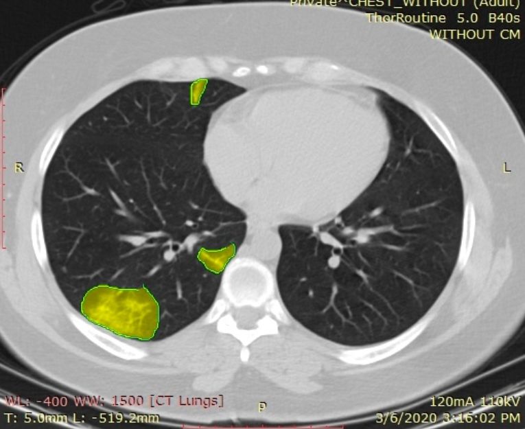
to community acquired pneumonia. The source code of our work is available at
https://github.com/DIAL-RPI/COVID19-ICUPrediction.
Keywords: COVID-19; Chest CT; Outcome Prediction; Artificial Intelligence.

1. Introduction

    Coronavirus disease 2019 (COVID-19), which results from contracting an
extremely contagious beta-coronavirus, is responsible for the latest pandemic
in human history. The resultant lung injury from COVID-19 pneumonia can
progress rapidly to diffuse alveolar damage, acute lung failure, and even death
(Vaduganathan et al., 2020; Danser et al., 2020). Given the highly contagious
nature of the infection, the burden of COVID-19 pneumonia has imposed sub-
stantial constraints on the global healthcare systems. In this paper, we present a
novel framework of integrative analysis of heterogeneous data including not only
medical images, but also patient demographic information, vital signs and lab-
oratory blood test results for assessing disease severity and predicting intensive
care unit (ICU) admission of COVID-19 patients. Screening out the high-risk
patients, who may need intensive care later, and monitoring them more closely
to provide early intervention may help save their lives.
    Reverse transcription polymerase chain reaction (RT-PCR) assay with de-
tection of specific nuclei acid of SARS-CoV-2 in oral or nasopharyngeal swabs
is the preferred test for diagnosis of COVID-19 infection. Although chest com-
puted tomography (CT) can be negative in early disease, it can achieve higher
than 90% sensitivity in detecting COVID-19 pneumonia but with low specificity
(Kim et al., 2020). For diagnosis of COVID-19 pneumonia, CT is commonly
used in regions with high prevalance and limited RT-PCR availability as well
as in patients with suspected false negative RT-PCR. CT provides invaluable
information in patients with moderate to severe disease to assess the severity
and complications of COVID-19 pneumonia (Yang et al., 2020). Prior clini-
cal studies with chest CT have reported that qualitative scoring of lung lobar
involvement by pulmonary opacities (high lobar involvement scores) can help
assess severe and critical COVID-19 pneumonia. Li et al. (2020a) showed that
high CT severity scores (suggestive of extensive lobar involvement) and con-
solidation are associated with severe COVID-19 pneumonia. Zhao et al. (2020)
reported that extent and type of pulmonary opacities can help establish severity
of COVID-19 pneumonia. The lung attenuation values change with the extent
and type of pulmonary opacities, which differ in patients with more extensive,
severe disease from those with milder disease. Most clinical studies focus on
qualitative assessment and grading of pulmonary involvement in each lung lobe
to establish disease severity, which is both time-consuming and associated with
interobserver variations (Zhao et al., 2020; Ai et al., 2020). To address the ur-
gent clinical needs, artificial intelligence (AI), especially deep learning, has been
applied to COVID-19 CT image analysis (Shi et al., 2020). AI has been used to
differentiate COVID-19 from community acquired pneumonia (CAP) on chest

                                         2
CT images (Li et al., 2020b; Sun et al., 2020). To unveil what deep learning
uses to diagnose COVID-19 from CT, Wu et al. (2020) proposed an explainable
diagnosis system by classifying and segmenting infections. Gozes et al. (2020b)
developed a deep learning based pipeline to segment lung, classify 2D slices and
localize COVID-19 manifestation from chest CT scans. Shan et al. (2020) went
on to quantify lung infection of COVID-19 pneumonia from CT images using
deep learning based image segmentation.
    Among the emerging works, a few AI based methods target at severity as-
sessment from chest CT. Huang et al. (2020) developed a deep learning method
to quantify severity from serial chest CT scans to monitor the disease progres-
sion of COVID-19. Tang et al. (2020) used random forest to classify pulmonary
opacity volume based features into four severity groups. By automatically seg-
menting the lung lobes and infection areas, Gozes et al. (2020a) suggested a
“Corona Score” to measure the progression of disease over time. Zhu et al.
(2020) further proposed to use AI to predict if a patient may develop severe
symptoms of COVID-19 and how long it may take if that is the case. Although
promising results have been presented, the existing methods primarily focus on
the volume of pulmonary opacities and their relative ratio to the lung volume
for severity assessment. The type of pulmonary opacities (e.g. ground glass,
consolidation, crazy-paving pattern, organizing pneumonia) is also an impor-
tant indicator of the stage of the disease and is often not quantified by the AI
algorithms (Chung et al., 2020).
    Furthermore, in addition to measuring and monitoring the progression of
severity, it could be life-saving to predict mortality risk of patients by learning
from the clinical outcomes. Since majority of the infected patients will recover,
managing the high-risk patients is the key to lower the fatality rate (Ruan,
2020; Phua et al., 2020; Li et al., 2020c). Longitudinal study analyzing the
serial CT findings over time in patients with COVID-19 pneumonia shows that
the temporal changes of the diverse CT manifestations follow a specific pattern
correlating with the progression and recovery of the illness (Wang et al., 2020).
Thus, it is promising for AI to perform this challenging task.
    In this paper, our objective is to predict outcome of COVID-19 pneumonia
patients in terms of the need for ICU admission with both imaging and non-
imaging information. The work has two major contributions.
  1. While image features have been commonly exploited by the medical image
     analysis community for COVID-19 diagnosis and severity assessment, non-
     imaging features are much less studied. However, non-imaging health data
     may also be strongly associated with patient severity. For example, Yan
     et al. (2020) showed that machine learning tools using three biomarkers,
     including lactic dehydrogenase (LDH), lymphocyte and high-sensitivity C-
     reactive protein (hs-CRP), can predict the mortality of individual patients.
     Thus, we propose to integrate heterogeneous data from different sources,
     including imaging data, age, sex, vital signs, and blood test results to
     predict patient outcome. To the best of our knowledge, this is the first
     study that uses holistic information of a patient including both imaging

                                        3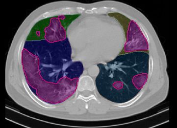
and non-imaging data for outcome prediction.
  2. In addition to the simple volume measurement based image features, ra-
     diomics features are computed to describe the texture and shape of pul-
     monary opacities. A deep learning based pyramid-input pyramid-output
     image segmentation algorithm is used to quantify the extent and volume
     of lung manifestations. A feature dimension reduction algorithm is further
     proposed to select the most important features, which is then followed by
     a classifier for prediction.
It is worth noting that although the presented application on COVID-19 pneu-
monia, the proposed method is a general approach and can be applied to other
diseases.
    The proposed method was evaluated on datasets collected from teaching
hospitals across three countries, These datasets included 113 CT images from
Firoozgar Hospital (Tehran, Iran)(Site A), 125 CT images from Massachusetts
General Hospital (Boston, MA, USA)(Site B), and 57 CT images from Univer-
sity Hospital Maggiore della Carita (Novara, Piedmont, Italy)(Site C). Promis-
ing experimental results for outcome prediction were obtained on all the datasets
with our proposed method, with reasonable generalization across the datasets.
Details of our work are presented in the following sections.

2. Datasets

    The data used in our work were acquired from three sites. All the CT imaging
data were from patients who underwent clinically indicated, standard-of-care,
non-contrast chest CT without intravenous contrast injection. Age and gender
of all patients were recorded. For datasets from Sites A and B, lymphocyte
count and white blood cell count were also available. For datasets of Sites A and
C, peripheral capillary oxygen saturation (SpO2) and temperature on hospital
admission were recorded. Information pertaining patient status (discharged,
deceased, or under treatment at the time of data analysis) was also recorded as
well as the number of days of hospitalization to the outcome.

Site A Dataset. We reviewed medical records of adult patients admitted with
known or suspected COVID-19 pneumonia in Firoozgar Hospital (Tehran, Iran)
between February 23, 2020 and March 30, 2020. Among the 117 patients with
positive RT-PCR assay for COVID-19, three patients were excluded due to
presence of extensive motion artifacts on their chest CT. With one patient who
neither admitted to ICU nor discharged, 113 patients are used in this study.

Site B Dataset. We reviewed medical records of adult patients admitted with
COVID-19 symptom in MGH between March 11 and May 3, 2020. 125 RT-PCR
positive admitted patients underwent unenhanced chest CT are selected to form
this dataset.

                                       4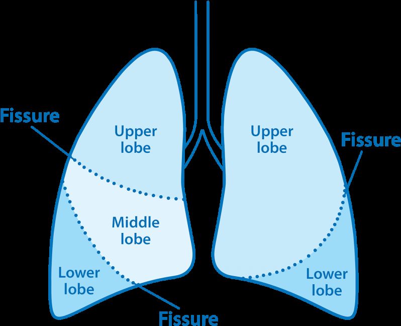
Vital Signals

       Chest CT Volume                                                             ICU admission
                                         Blood Test                                  prediction
                   Segmentation
   Segmentation

                    Pulmonary
                     Opacities

                                                                                       Positive
       Lobe

                                                                   Random Forest
                                     Demographic Data

                                      Whole Lung Radiomics
                                                                                       Negative

                  Hierarchical Lobe-wise Quantification Features

Figure 1: Framework of the proposed methods including the utilized inputs and expected
output.

Site C Dataset. We reviewed medical records of adult patients admitted with
COVID-19 pneumonia in the Novara Hospital (Piedmont, Italy) between March
4, 2020 and April 6, 2020. We collected clinical and outcome information of 57
patients with positive RT-PCR assay for COVID-19.
    Two experienced thoracic subspecialty radiologists evaluated all chest CT
examinations and recorded opacity type, distribution and extent of lobar in-
volvement. Information on symptom duration prior to hospital admission, du-
ration of hospital admission, presence of comorbid conditions, laboratory data,
and outcomes (recovery or death) was obtained from the medical records. En-
tire lung volume was segmented on thin-section DICOM images (1.5-2 mm) to
obtain whole-lung analysis. Statistics of the datasets are shown in Tables 3-5 in
Section 3.4.

3. ICU Admission Prediction

    In order to predict the need for ICU admission of patients with COVID-
19 pneumonia, we use three types of imaging and non-imaging features. Our
adopted features include hierarchical lobe-wise quantification features (HLQ),
whole lung radiomics features (WLR), and features from demographic, vital
signs, and blood examination (DVB). Figure 1 shows an overview of the overall
framework of the presented work. In the rest of this section, we first introduce
the details of these features. Since it is challenging to fuse the large number

                                                         5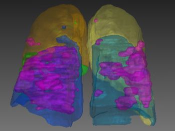
(a) COVID-19 CT image           (b) Lobes and infection         (c) 3D Visualization

Figure 2: Lung lobes and pulmonary opacities segmentation results. Areas colored in magenta
indicate the segmented lesions.

of inhomogeneous features together, a feature selection strategy is proposed,
followed by random forest based classification (Breiman, 2001).

3.1. Deep Learning based Image Segmentation
    In our work, we employed deep neural networks to segment both lungs, five
lung lobes and pulmonary opacities (as regions of infection) from non-contrast
chest CT examinations. For training purpose, we semi-automatically labeled 71
CT volumes using 3D Slicer (Kikinis et al., 2014). For lung lobe segmentation,
we adopted the automated lung segmentation method by Hofmanninger et al.
(2020). The pre-trained model1 was fine-tuned with a learning rate of 1 × 10⁻⁵
using our annotated data. The tuned model was then applied to segment all
the chest CT volumes.
    Segmentation of pulmonary opacities was completed by our previously pro-
posed method, Pyramid Input Pyramid Output Feature Abstraction Network
(PIPO-FAN) (Fang and Yan, 2020) with publicly released source code2 .
    Figure 2 shows the segmentation results of lung lobes and pulmonary opac-
ities. From axial and 3D view, we can see that the segmentation models can
smoothly and accurately predict isolate regions with pulmonary opacities.

3.2. Hierarchical Lobe-wise Quantification Features
    Based on the segmentation results in Section 3.1, we then compute the ratio
of opacity volume over different lung regions, which is a widely used measure-
ment to describe the severity (Tang et al., 2020; Zhu et al., 2020). The lung
regions include the whole lung, the left lung and the right lung and 5 lung lobes
(lobe# 1-5) as shown in Figure 2. The right lung includes upper lobe (lobe#
1) , middle lobe (lobe# 2), and lower lobe (lobe# 3), while left lung includes
upper lobe(lobe# 4) and lower lobe (lobe# 5). Thus, each CT image has 8
regions of interest (ROIs). In addition to the ROI segmentation, we partitioned
each segment to 4 parts based on the HU ranges, i.e., the HU ranges of -∞ to

  1 https://github.com/JoHof/lungmask
  2 https://github.com/DIAL-RPI/PIPO-FAN

                                            6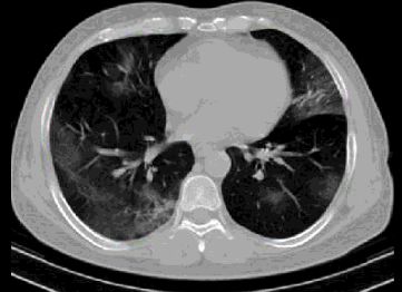
Table 1: Radiomics feature types and number of each kind of features.

               Group       Feature type         # features       Sum
                           First order              18
                           GLCM                     24
                           GLRLM                    16
               Texture                                            93
                           GLSZM                    16
                           NGTDM                    5
                           GLDM                     14
               Shape       Shape (3D)               17            17

-750 (HU[-∞, -750]), -750 to -300 (HU[-750, -300]), -300 to 50 (HU[-300, 50]),
and 50 to +∞ (HU[50, +∞]). These four HU ranges correspond to normal
lungs, ground glass opacity (GGO), consolidation, and regions with pulmonary
calcification, respectively. As a result, each CT image was partitioned to 32
components (8 ROIs × 4 ranges/ROI).
    We extracted two quantitative features from each part, i.e., volumes of pul-
monary opacities (VPO) and ratio of pulmonary opacities to the corresponding
component (RPO), as defined below:

                           V P O(x) = V (Segment(x))                             (1)

                                  V P O(x)   V (Segment(x))
                    RP O(x) =              =                                     (2)
                                    V (x)         V (x)
where x is a selected component (among the 32 components). Segment(x)
denotes the pulmonary opacities in the selected component x based on the
segmentation of pulmonary opacities in Figure 2. V (·) denotes the volume of
the selected part.

3.3. Whole Lung Radiomics Features
    To more comprehensively describe information in the CT image, we also
extracted multi-dimensional radiomics features (Gillies and Kinahan, 2015) of all
pulmonary opacities. Compared with HLQ feature, although they are all image-
based features, they describe the pulmonary opacities from different aspects.
HLQ features focus on the pulmonary opacities volume and position of region
of interest, while WLR focus on their shape and texture.
    For each chest CT volume, we first masked out non-infection regions based
on the infection segmentation results, then four kinds of radiomics features are
calculated on the volume, i.e., shape, first-order, second-order and higher-order
statistics features (Rizzo et al., 2017). Shape features describe the geomet-
ric information. First-order, second-order and higher-order statistics features
all describes texture information. First-order statistics features describe the
distribution of individual voxel values without concerning spatial correlation.
Second-order features describe local structures, which provide correlated in-
formation between adjacent voxels and statistical measurement of intra-lesion

                                          7
Table 2: Image filter types and extracted radiomics features from each type of filtered images.
Image filter type Extracted features # features
No filter (Original image) Texture + Shape 93+17=110
Square filter Texture 93
Square-root(Sqrt) filter Texture 93
Logarithm filter Texture 93
Exponential filter Texture 93
Wavelet filters
(HHH, HHL, HLH, LHH, Texture 93×8=744
HLL, LHL, LLH, LLL)
Laplacian of Gaussian (LoG) filters
Texture 93×5=465
σ ∈ {0.5, 1.5, 2.5, 3.5, 4.5}
heterogeneity. Second-order features include those extracted using gray level
dependence matrix (GLDM), gray level co-occurrence matrix (GLCM), grey
level run length matrix (GLRLM), grey level size zone matrix (GLSZM), and
neighboring gray tone difference matrix (NGTDM). Higher-order statistics fea-
tures are computed using the same methods as second-order features but af-
ter applying wavelets and Laplacian transform of Gaussian(LoG) filters. The
higher-order features help identify repetitive patterns in local spatial-frequency
domain in addition to suppressing noise and highlighting details of images.
We used the Pyradiomics package (Griethuysen et al., 2017) to extract the
above described radiomics features from COVID19 chest CT images. For each
chest CT volume, a total of 1691 features are extracted. The number of ra-
diomics features for each feature type are summarized in Table 1. Based on the
description above, these features can be categorized into two main groups, i.e.,
17 shape features and 93 texture features.
To extracted various features, different image filters are applied before fea-
ture extraction. Table 2 shows the details of all 18 image filter types used in our
work, including no filter, square filter, square-root filter, logarithm filter, expo-
nential filter, wavelet filter and LoG filter. The image filtered by a 3D wavelet
filter has eight channels, including HHH, HHL, HLH, LHH, HLL, LHL, LLH and
LLL. The Laplacian of Gaussian (LoG) filters have a hyper-parameter σ which
is the standard deviation of the Gaussian distribution. We used five different
σ values in our study, i.e., {0.5, 1.5, 2.5, 3.5, 4.5}. Note that shape features are
only extracted from the original images (no filter was applied).
3.4. Non-imaging Features
In addition to features extracted from images, we incorporated features from
demographic data (contained by all three datasets), vital signs (from Sites A and
B), and laboratory data (from Sites A and C) (DVB). Specifically, such features
include patients’ age, gender, white blood cell count (WBC), lymphocyte count
(Lym), Lym to WBC ratio (L/W ratio), temperature and blood oxygen level
(SpO2). These data are highly correlated with the ICU admission of patients
8Table 3: Statistics (mean±std, except for gender) of DVB features for Site A dataset.
ICU admission Not Admitted ICU Admitted Data #
Gender (M:F) 43 : 28 29 : 13 113
Age (year) 56.7 ± 16.0 66.9 ± 16.2 113
Lym r (%) 22.7 ± 8.3 15.6 ± 12.8 113
WBC 5831.0 ± 1848.9 7966.7 ± 4556.2 113
Lym 1244.7 ± 482.8 1010.4 ± 943.7 113
Temperature (℃) 37.3 ± 0.6 37.6 ± 0.6 98
SpO2 (%) 91.9 ± 7.41 86.5 ± 8.53 100
Table 4: Statistics (mean±std, except for gender) of DVB features for Site B dataset.
ICU admission Not Admitted ICU Admitted Data #
Gender (M:F) 23 : 24 39 : 39 125
Age (year) 74.8 ± 15.0 72.7 ± 11.1 125
Lym r (%) 18.6 ± 12.7 13.0 ± 12.8 125
WBC 7175.7 ± 4288.9 11722.3 ± 7249.3 125
Lym 1058.1 ± 596.7 1613.8 ± 3872.7 125
when they were admitted to a hospital. Table 3-5 show the statistics of the
above features in Site A, Site B, and Site C datasets respectively. Non-imaging
features are not all available for some patients. The number of the collected
data for each feature is listed in the last column of the tables. To make use
of all the data, the missing values are imputed by the mean values of other
available entries. For instance, in Site A dataset, if a patients SpO2 was not
recorded, the mean SpO2 value of 91.9 from the dataset is used to fill the blank.
3.5. ICU Admission Prediction
In our work, random forest (RF) (Breiman, 2001) classifier, a widely-used
ensemble learning method consisting of multiple decision trees, is chosen for
predicting ICU admission due to its several nice properties. First, RF is robust
to small data size. Second, it can generate feature importance ranking and is
thus highly interpretable. Aggregating all the features introduced above, we
have 1,762 features in total. Due to the limited data size, the model would
easily overfit with all features as input. Thus, we first used RF to rank all the
features, then we selected the top K features for our final prediction.
We ranked the feature based on their Gini importance (Leo et al., 1984). It is
calculated during the training of RF by averaging the decrease of Gini impurity
Table 5: Statistics (mean±std, except for gender) of DVB features for Site C dataset.
ICU admission Not Admitted ICU Admitted Data #
Gender (M:F) 13 : 8 24 : 12 57
Age (year) 70.0 ± 13.7 66.9 ± 12.3 57
Temperature (℃) 39.0 ± 1.0 37.8 ± 0.9 50
SpO2 (%) 92.3 ± 5.25 84.5 ± 7.74 31
9Cross Entropy Loss
Concatenate
Dropout
Dropout 16
Dropout
Auxiliary
8
CE Loss
Dropout
Auxiliary
CE Loss Dropout
16 16 16 16
16
16
Dropout
Auxiliary
CE Loss
64 17 324 375 975
Non-imaging Features Hierarchical Lobe-wise Whole Lung Radiomics Features
Quantification Features
Shape First Order Second Order High Level
Figure 3: Architecture of the Wide & Deep Net (Cheng et al., 2016) based deep neural
network (DNN). Three different kinds of features are first processed separately by one or two
fully connected layers. Then the learned features are concatenated for the final prediction.
over all trees. Due to the randomness of RF, Gini importance of features may
vary when RF model is initialized with different random seeds. Therefore, in
our study, feature ranks are computed 100 times with different random seeds.
Each time every feature will get a score being its rank. The final feature rank
is obtained by sorting the total summed score of each feature.
Based on the rank of all the features, we select top K ∈[1,100] features to
train the RF model and calculate the prediction performance in terms of AUC.
4. Experimental Results
This section presents the experimental results of the developed methods. We
show the effectiveness of our proposed method on the three datasets separately
through both ablation studies and comparison with other state-of-the-art ap-
proaches. We did not merge the datasets because of two reasons. First, not all
the non-image features were available from the participating sites. Second, the
treatment and admission criteria at the participating sites were likely different
from each other. Given such limitations, the datasets were used separately to
evaluate the proposed methods.
The experiments are summarized in to two parts. In the first part, the pro-
posed methods with different combinations of features is compared with other
state-of-the-art approaches on each dataset. In this part of the experiments,
we also included results of support vector machine (SVM), logistic regression
and three other deep learning networks. The first deep neural network (DNN)
takes all the WLR, HLQ and DVB features as its input and consists of three
fully connected layers with output dimensions of 64, 16 and 2 respectively (de-
noted as DNN w/ all features). Dropout was applied on the first two layers
with 50% dropping rate. The second deep network takes features selected by
random forest as its input. As the selected features is only a small subset of all
10the features, this network is smaller than the first one. It contains three fully
connected layers with output dimension of 8, 8 and 2, respectively (denoted as
DNN (small)). The third network is designed based on the Wide & Deep Net
(WD Net) (Cheng et al., 2016) to investigate whether a more complex network
could perform better directly using all features as an input (denoted as WD
Net w/ all features). The detailed structure is shown in Fig. 3. For all the
three networks, the cross entropy loss is used for training. For a sample with
label y ∈ {0, 1}, the cross entropy loss is formulated as l = −logPy , where Py
is the output prediction probability of class y. In the five-fold cross valida-
tion scheme, each time 3 folds are used to train the network, one fold is used
as validation set, and the last one is reserved as test set. The networks were
implemented over PyTorch (Paszke et al., 2019) and trained using the Adam
optimizer with learning rate of 1e − 4. Influenced by the size of dataset and
the network, the WD Net on Site B dataset took the longest time for training
which is 3.0 min with 4 NVIDIA Tesla V100 GPUs. In the second part of the
experiments, the generalization ability of the feature combination learned by our
model is studied across three datasets. The code is open sourced and available
at https://github.com/DIAL-RPI/COVID19-ICUPrediction.
Several recent works have shown the importance of using machine learning
models to predict patients’ outcomes based on lobe-wise quantification features.
The infection volume and infection ratio of the whole lung, right/left lung, and
each lobe/segment are calculated as quantitative features in Tang et al. (2020).
Random forest classifier is used to select the top-ranking features and make
the severity assessment based on these features. In another work by Zhu et al.
(2020), the authors present a novel joint regression and classification method
to identify the severity cases and predict the conversion time from a non-severe
case to the severe case. Their lobe-wised quantification features include the
infection volume, density feature and mass feature. As we mentioned earlier, all
existing image analysis-based outcome prediction works use only image features.
We take the features in the two papers as baseline to compare with our work.
4.1. Results on Site A Dataset
Table 6: Comparison among the features used in exist state-of-the-art works and different
combinations of the proposed features on ICU admission prediction on Site A dataset. One-
tailed t-test is used to evaluate the statistical significance between a feature combination and
the best performer.
AUC Sensitivity (PPV=70%)
Features K
Mean 95% CI p Value Mean 95% CI p Value
Img feature (Tang 2020) 0.818 (0.796, 0.839) p < .001 51.0% (39.3%, 62.6%) p < .001 8
Img feature (Zhu 2020) 0.776 (0.762, 0.790) p < .001 48.6% (35.4%, 61.7%) p = .001 46
DVB 0.855 (0.844, 0.866) p = .002 76.7% (73.2%, 80.1%) p = .017 1
HLQ 0.789 (0.781, 0.797) p < .001 51.4% (45.3%, 57.5%) p < .001 21
WLR 0.859 (0.843, 0.873) p < .001 71.4% (60.5%, 82.3%) p = .022 70
WLR+HLQ 0.866 (0.857, 0.875) p < .001 68.6% (57.6%, 79.5%) p = .008 61
WLR+DVB 0.876 (0.867, 0.886) p=.109 81.4% (76.0%, 86.8%) p=.152 4
HLQ+DVB 0.865 (0.844, 0.885) p=.080 70.0% (60.9%, 79.1%) p = .012 4
WLR+HLQ+DVB 0.884 (0.875, 0.893) - 84.3% (79.9%, 88.7%) - 52
111.0
0.8
0.6
Sensitivity
Chance
0.4 Baseline2 (AUC = 0.78±0.01)
Baseline1 (AUC = 0.82±0.02)
HLQ+DVB (AUC = 0.86±0.02)
WLR+HLQ (AUC = 0.87±0.01)
0.2 WLR+DVB (AUC = 0.88±0.01)
WLR (AUC = 0.86±0.01)
HLQ (AUC = 0.79±0.01)
DVB (AUC = 0.85±0.01)
0.0 WLR+HLQ+DVB (AUC = 0.88±0.01)
0.0 0.2 0.4 0.6 0.8 1.0
1-Specificity
Figure 4: ROC curves of various feature combinations on Site A dataset. DVB: non-imaging
features including Demographic data, Vital signals and Blood test results; HLQ: Hierarchical
Lobe-wise Quantification features; WLR: Whole Lung Radiomics features.
Receiver Operating Characteristics (ROC) curves of the feature combina-
tions are shown in Figure 4. For each feature combination, the features are
selected only from the feature categories available in the combination using the
approach introduced in Section 3.5. For example, HLQ+DVB indicates that
only features from these two groups, HLQ and DVB, are selected and used.
The number of features K used to obtain the best results are listed in Table 6.
To alleviate the stochasticity of the results, for each feature combination, five
RF models with different random seeds are trained and tested with five fold
cross validation. The curves shown here are thus the mean results of the five
models. The figure legend gives the mean Area Under the Curves (AUCs) of
the feature combinations as well as the standard deviation (mean±std). It can
be seen that the combination of all three kinds of features, WLR+HLQ+DVB,
obtained the best result with an AUC of 0.88±0.01. The variation of AUC along
with number of selected features on Site A dataset is presented in Fig. 5. As
marked by the light blue dash line in Fig. 5, AUC reaches the maximum value
when the top 52 features are selected. Details of the 52 selected features are
presented in Table 15 at the end of this paper due to its large size.
One-tailed t-test is used to evaluate the statistical significance between a
method and the best performer. Table 6 summarizes the AUC values and sen-
sitivity with significance test p values and 95% confidence interval (95% CI).
The classification threshold is selected by control the positive prediction value
(PPV) to be 70%. The combination of WLR+HLQ+DVB significantly exceeds
other reported methods (Tang et al., 2020; Zhu et al., 2020) with p ≤ 0.001.
120.89
0.88
0.87
AUC 0.86
0.85
WLR+HLQ+DVB
0.84
Max AUC, Feature# = 52
0.83
0 20 40 60 80 100
Number of Selected Features
Figure 5: Variation of AUC along choosing the top K features.
Further, we achieved a sensitivity of 84.3% while retaining a PPV at 70%. It
suggests that our model can rapidly prioritize over 80% patients who would
develop into critical conditions, if we allow 3 false positive cases in every 10
positive predictions. With such prediction, hospitals may allocate limited med-
ical resources more efficiently to potentially prevent such conversion and save
more lives. Under the same setting, the sensitivity of the model is 79.4%, the
accuracy is 81.2%.
Table 7: Comparison of different machine learning methods with selected features on Site A
dataset. One-tailed t-test is used to evaluate the statistical significance between a feature
combination and the best performer.
AUC Sensitivity (PPV=70%)
Methods
Mean 95% CI p Value Mean 95% CI p Value
Random Forests 0.884 (0.875, 0.893) - 84.3% (79.9%, 88.7%) -
SVM 0.867 (0.855, 0.880) p = .002 71.0% (64.9% , 77.0%) p < .001
Logistic Regression 0.785 (0.758, 0.812) p < .001 31.0% (14.8%, 47.1%) p < .001
DNN (small) 0.816 (0.804, 0.828) p < .001 - - p = 0.023
DNN w/ all features 0.751 (0.723, 0.779) p < .001 25.7% (0.8%, 50.6%) p = .003
WD Net w/ all features 0.823 (0.807, 0.838) p < .001 58.1% (40.7%, 75.5%) p = .009
In the comparison among different combinations of the features, we can
see that the results are generally improved with more feature sources added.
Comparison between WLR+HLQ (line 6) and WLR+HLQ+DVB (the last line)
shows that, on this dataset, introducing non-imaging features can significantly
improve the performance (pof DNN (small) is not included because it couldnt obtain a PPV equal or larger
than 70% in some of the cross validation folds.
4.2. Results on Site B Dataset
Table 8: Comparison among the features used in exist state-of-the-art works and different
combinations of the proposed features on ICU admission prediction on Site B dataset.
AUC Sensitivity (PPV=70%)
Features K
Mean 95% CI p Value Mean 95% CI p Value
Img feature (Tang 2020) 0.770 (0.745, 0.796) p < .001 83.1% (75.8%, 90.4%) p = .009 10
Img feature (Zhu 2020) 0.767 (0.752, 0.781) p < .001 83.8% (82.2%, 85.5%) p < .001 39
DVB 0.671 (0.643, 0.700) p < .001 78.7% (69.7%, 87.7%) p = .007 4
HLQ 0.791 (0.774, 0.809) p < .001 84.6% (81.3%, 88.0%) p < .001 3
WLR 0.841 (0.827, 0.855) p = .014 94.9% (93.4%, 96.3%) - 55
WLR+HLQ 0.847 (0.833, 0.861) - 92.6% (89.5%, 95.7%) p = .083 12
WLR+DVB 0.841 (0.828, 0.854) p = .257 91.8% (90.5%, 93.1%) p = .012 33
HLQ+DVB 0.796 (0.777, 0.815) p = .001 84.4% (80.7%, 88.0%) p < .001 4
WLR+HLQ+DVB 0.844 (0.833, 0.855) p = .310 92.6% (90.0%, 95.1%) p = .027 12
1.0
0.8
0.6
Sensitivity
Chance
0.4 Baseline2 (AUC = 0.72±0.02)
Baseline1 (AUC = 0.77±0.05)
WLR+HLQ+DVB (AUC = 0.85±0.03)
WLR+HLQ (AUC = 0.86±0.02)
0.2 WLR+DVB (AUC = 0.86±0.04)
WLR (AUC = 0.85±0.04)
HLQ (AUC = 0.77±0.03)
DVB (AUC = 0.58±0.06)
0.0 HLQ+DVB (AUC = 0.85±0.04)
0.0 0.2 0.4 0.6 0.8 1.0
1-Specificity
Figure 6: ROC curves on Site B dataset.
The same set of experiments were repeated on the Site B dataset. Table 8
and Fig. 6 shows the results. The number of features K used to obtain the best
results for each combination are listed in Table 8. It can be seen that, on Site
B dataset, non-imaging features are not very predictive. There could be several
reasons for the inability of DVB features on Site B dataset. First, as shown in
Table. 4 non-imaging features on Site B dataset have a large standard deviation.
Second, the use of CT in Site B is different from that in Site A. Site B relied
on chest radiography for most patients while CT was reserved for more sicker
14Table 9: The top 12 WLR+HLQ features ranked by feature ranking strategy introduced in
Section 3.5 on Site B dataset. The third and sixth columns show the Gini importance of the
corresponding feature averaged in the 5-fold cross validation.
# Quantitative features G(%) # Quantitative features G(%)
1 Lobe#2 RPO HU3 10.27 2 Lobe#2 RPO HU2 8.45
3 Whole Lung RPO HU1 10.77 4 LoG(σ = 4.5)-firstorder-Kurtosis 7.74
5 Exponential-GLRLM-ShortRunLowGL 7.8 6 LoG(σ = 4.5)-NGTDM-Contrast 8.07
7 Exponential-GLRLM-ShortRun 7.24 8 LoG(σ = 3.5)-GLSZM-ZoneEntropy 7.58
9 LoG(σ = 4.5)-NGTDM-Busyness 7.0 10 Sqrt-NGTDM-Strength 9.0
11 LoG(σ = 3.5)-GLCM-Imc2 8.17 12 LLH-GLSZM-GLNonUnif 7.89
Green text indicates lobe-wise quantification features, HU1-HU4 are the four HU intervals.
Blue text indicates whole lung radiomics features encoded as Filter-FeatureType-
Parameter.
patients or those with suspected complications; Site A used CT in all patients
regardless of clinical severity. Third, criteria of ICU admission are different
between two sites. Fourth, management strategies and disease outcomes at the
two sites are different.
Table 10: Comparison of different machine learning methods with selected features on Site B
dataset.
AUC Sensitivity (PPV=70%)
Methods
Mean 95% CI p Value Mean 95% CI p Value
Random Forests 0.844 (0.833, 0.855) - 92.6% (90.0%, 95.1%) -
SVM 0.852 (0.838, 0.866) p = .148 95.4% (93.2% , 97.5%) p = .020
Logistic Regression 0.798 (0.783, 0.812) p = .003 90.2% (88.6%, 91.9%) p = .110
DNN (small) 0.831 (0.805, 0.858) p = .187 86.9% (83.5%, 90.3%) p = .003
DNN w/ all features 0.704 (0.670, 0.738) p < .001 75.38% (71.6%, 79.2%) p = .001
WD Net w/ all features 0.769 (0.753, 0.786) p < .001 85.6% (82.6%, 88.7%) p = .004
In this experiment, the best AUC value, 0.847, is achieved by merging two
image-based feature, i.e., WLR+HLQ (line 6). With 70% PPV, WLR+HLQ
obtained a sensitivity of 92.6%, a specificity of 37.0% and an accuracy of 71.7%.
The best sensitivity (with PPV=70%), 94.9% is obtained by WLR features.
Although the sensitivity of WLR is higher than WLR+HLQ, there is no signif-
icant difference (p = 0.083 > 0.05). Table 9 lists the 12 WLR+HLQ features
used to obtain the best results. Table 10 shows the results of different methods
on Site B dataset. Three traditional machine learning methods and the DNN
(small) model used the 12 selected WLR+HLQ+DVB features (listed in Ta-
ble 11) for prediction. SVM achieved the best AUC and sensitivity. Random
forest obtained competitive AUC value with no significant difference (p > 0.05)
but inferior sensitivity (p < 0.05). The DNN (small) model here also achieved
an AUC value comparable with the best result but much lower sensitivity.
4.3. Results on Site C Dataset
Results on Site C dataset are shown in Table 12 and Fig. 6. The non-imaging
(DVB) features alone also didn’t achieve well performance. It might be because
many petients’ DVB features are missing or incomplete as shown in Table. 5
Yet, the introduce of DVB features significantly improves the AUC performance
15Table 11: The 12 best WLR+HLQ+DVB features used for the experiments in Table 10 ranked
by feature ranking strategy introduced in Section 3.5 . The third and sixth columns show the
Gini importance of the corresponding feature averaged in the 5-fold cross validation.
# Quantitative features G(%) # Quantitative features G(%)
1 Lobe#2 RPO HU3 9.90 2 WBC 8.24
3 Lobe#2 RPO HU2 8.85 4 Whole Lung RPO HU4 8.78
5 LoG(σ = 4.5)-Firstorder-Kurtosis 7.6 6 Exponential-GLRLM-ShortRunLowGL 7.79
7 Exponential-GLRLM-ShortRun 7.48 8 Sqrt-NGTDM-Strength 9.17
9 LoG(σ = 3.5)-GLSZM-ZoneEntropy 7.91 10 Right Lung RPO HU4 8.0
11 LLL-NGTDM-Strength 7.79 12 LoG(σ = 4.5)-NGTDM-Contrast 8.51
Red text indicates non-imaging features.
Green text indicates lobe-wise quantification features, HU1-HU4 are the four HU intervals.
Blue text indicates whole lung radiomics features encoded as Filter-FeatureType-
Parameter.
Table 12: Comparison among the features used in exist state-of-the-art works and different
combinations of the proposed features on ICU admission prediction on Site C dataset.
AUC Sensitivity (PPV=70%)
Features K
Mean 95% CI p Value Mean 95% CI p Value
Img feature (Tang 2020) 0.763 (0.670, 0.856) p = .044 85.0% (76.4%, 93.6%) p = .020 10
Img feature (Zhu 2020) 0.675 (0.645, 0.706) p < .001 73.9% (59.0%, 88.8%) p < .011 39
DVB 0.595 (0.524, 0.665) p < .001 63.3% (36.1%, 90.5%) p = .019 4
HLQ 0.691 (0.660, 0.722) p < .001 86.7% (80.3%, 93.0%) p < .014 7
WLR 0.815 (0.782, 0.848) p = .020 95.6% (92.8%, 98.3%) p = .186 12
WLR+HLQ 0.826 (0.813, 0.839) p = .191 96.1% (94.4%, 97.8%) - 20
WLR+DVB 0.835 (0.809, 0.861) p = .365 95.0% (91.6%, 98.4%) p = .088 15
HLQ+DVB 0.760 (0.705, 0.815) p = .016 85.6% (77.6%, 93.5%) p < .010 2
WLR+HLQ+DVB 0.840 (0.804, 0.876) - 94.4% (92.3%, 96.6%) p = .035 35
1.0
0.8
0.6
Sensitivity
Chance
0.4 Baseline2 (AUC = 0.68±0.03)
Baseline1 (AUC = 0.76±0.08)
DVB (AUC = 0.59±0.06)
HLQ (AUC = 0.69±0.03)
0.2 WLR (AUC = 0.81±0.03)
WLR+DVB (AUC = 0.84±0.02)
WLR+HLQ (AUC = 0.83±0.01)
HLQ+DVB (AUC = 0.76±0.05)
0.0 WLR+HLQ+DVB (AUC = 0.84±0.03)
0.0 0.2 0.4 0.6 0.8 1.0
1-Specificity
Figure 7: ROC curves on Site C dataset.
16Table 13: Comparison of different machine learning methods with selected features on Site C
dataset.
AUC Sensitivity (PPV=70%)
Methods
Mean 95% CI p Value Mean 95% CI p Value
Random Forests 0.840 (0.804, 0.876) - 94.4% (92.3%, 96.6%) -
SVM 0.811 (0.782, 0.839) p = .031 93.3% (89.2% , 97.5%) p = .324
Logistic Regression 0.717 (0.666, 0.768) p = .009 86.7% (79.3%, 94.0%) p = .019
DNN (small) 0.695 (0.619, 0.771) p = .011 77.8% (53.6%, 100.0%) p = .082
DNN w/ all features 0.568 (0.550, 0.587) p < .001 52.8% (29.2%, 76.4%) p = .006
WD Net w/ all features 0.528 (0.479, 0.578) p < .001 34.4% (24.1%, 44.8%) p < .001
of HLQ features (p = 0.014 < 0.05). In this experiment, the best AUC value,
0.840, is achieved by merging all three kinds of features. While maintaining
a PPV of 70%, it achieved a sensitivity of 94.4%, a specificity of 33.3% and
an accuracy of 71.9%. Table 16 shows the 35 features used to obtain the best
results at the end of this paper due to its large size. A comparison of different
methods on Site C dataset is shown in Table 13. Random forest obtained the
best AUC and sensitivity. The performance of all three deep learning networks
is less than adequate. One of the most important reasons may be that Site C
dataset is considerably smaller than the other two datasets (only containing 57
cases). Compared with traditional machine learning methods, the number of
parameters in deep learning models is several orders of magnitude larger, which
makes them much more vulnerable to overfitting with a limited training set.
4.4. Generalization Ability
In this section, we further evaluate if feature combinations learned from one
site can be generated to other sites. Experiments on all 6 permutations are
conducted (train on Site A, test on Site B; train on Site A, test on Site C; train
on Site B, test on Site A; train on Site B, test on Site C; train on Site C, test
on Site A; train on Site C, test on Site B). Considering the 3 datasets contains
differet DVB features, WLR+HLQ features are used in this section. The results
are shown in Table 14.
Table 14: Transferring WLR+HLQ features across the three datasets.
Methods A→B A→C B→A B→C C→A C→B Mean
Random Forests 0.740 (36) 0.685 (29) 0.754 (12) 0.633 (11) 0.591 (17) 0.717 (20) 0.687
SVM 0.774 (1) 0.686 (23) 0.777 (3) 0.710 (1) 0.649 (17) 0.694 (3) 0.715
Logistic Regression 0.744 (11) 0.706 (23) 0.756 (1) 0.698 (1) 0.642 (19) 0.752 (3) 0.716
There were tremendous differences in the geographic distribution and scan-
ner technologies used for imaging patients at the three participating sites. De-
spite this, we achieved AUC values as high as 0.777 for WLR+HLQ features.
Some variations in the AUCs and performance of our model across different
sites is expected due to challenges associated with acquisition of consistent data
variables and practices. The results in Table 14 shows that SVM and logistic
regression achieved very similar performance on average with no significant dif-
ference (p = 0.462).Although random forest did not perform well in this transfer
17experiment, the difference between random forest and SVM was not significant
(p = 0.058 > 0.05) either. Considering that Random Forest outperformed lo-
gistic regression on all three datasets as presented in Section 4.1-4.3, it is still
the overall best performing method in our study.
Our study stresses the need to combine imaging findings with clinical, lab-
oratory and management variables which can improve the model performance,
aid in better performance statistics on each dataset. On the other hand, com-
plexities of disease and its outcomes are tied to local factors and stress the
importance of tweaking the best models based on rich local or institutional
level factors rather than a single one-type-fit-all model.
5. Discussion and Conclusions
In this paper, we propose to combine size and volume information of the
lungs and manifestations, radiomics features of pulmonary opacities and non-
imaging DVB features to predict need for ICU admission in patients with
COVID-19 pneumonia. Metrics related to ICU admission rates, need and avail-
ability are key markers in management of individual patients as well as in re-
source planning for managing high prevalence diseases. To the best of our
knowledge, this is the first study that uses holistic information of a patient
including both imaging and non-imaging data to predict patient outcome.
Although promising results were achieved, the study has a few limitations.
First of all, due to the limited size of our datasets, we could not conduct more
fine-grained outcome predictions. The size of the available datasets could also
be the reason that more complex models, such as deep neural networks, did
not perform well in our experiments. Once larger datasets are available, our
model can be rapidly adapted to assess generalization ability and to establish
implications on datasets from other sites. Efforts are underway (such as within
Radiological Society of North America) to establish such imaging datasets of
COVID-19 pneumonia. Second, variations in performance of different imaging
and clinical features on datasets from three sites underscore the need for careful
local vetting of deep learning predictive models. Future models should take into
account regional bias introduced from different criteria on imaging use, under-
lying patient comorbidities, and management strategies, so that more robust
models can be built. This also goes beyond the generalization ability of ma-
chine learning in medical applications. The best and most relevant results likely
require regional, local or even site-specific tuning of predictive models. This
is especially true in context of the three sites, which are under very different
healthcare systems as in our study. We believe that this limitation is not unique
to our model. Last but not the least, another limitation of our study pertains
to the lack of access to the specific treatment regimens at the three sites; their
inclusion could have further enhanced the accuracy of our algorithm. However,
it also suggests that this generic approach can be trained on data from a hospital
to create a customized predictive model for clinical decision support.
In summary, our integrative analysis machine learning based predictive model
can help assess disease burden and forecast meaningful patient outcomes with
18Table 15: The top 52 features ranked by feature ranking strategy introduced in Section 3.5 on
Site A dataset. The third and sixth columns show the Gini importance of the corresponding
feature averaged in the 5-fold cross validation.
# Quantitative features G(%) # Quantitative features G(%)
1 L/W ratio 7.83 2 Sqrt-NGTDM-Strength 2.68
3 LLL-GLDM-LowGray 2.15 4 Lobe#5 RPO HU4 2.27
5 Org-GLDM-LowGray 1.85 6 Lobe#5 RPO HU3 2.03
7 LLL-GLRLM-LongRunLG 1.71 8 Left Lung RPO HU4 2.16
9 Lym count 2.62 10 Lobe#2 VPO HU3 1.7
11 Lobe#2 VPO HU2 1.78 12 LLL-GLRLM-LGRun 2.23
13 LoG(σ = 1.5)-GLCM-MCC 3.04 14 LLL-GLSZM-LGZone 1.8
15 Org-NGTDM-Strength 1.71 16 Lobe#5 VPO HU3 1.82
17 Org-GLRLM-ShortRunLG 1.34 18 LLL-NGTDM-Strength 1.63
19 Org-GLRLM-LowGrayRun 1.43 20 LLL-GLDM-LargeDepdLG 1.94
21 LLL-GLRLM-ShortRunLG 1.73 22 LLL-GLSZM-SmallAreaLG 1.39
23 LLL-GLSZM-SmallAreaHG 1.93 24 LoG(σ = 2.5)-GLCM-MCC 2.62
25 WBC 1.81 26 Org-Shape-LeastAxisLength 1.57
27 Org-GLRLM-LongRunLG 1.22 28 LoG(σ = 1.5)-GLCM-Corr 2.54
29 Lobe#2 Infection Ratio HU4 1.4 30 HLL-FirstOrder-Mean 1.91
31 Left Lung VPO HU2 1.51 32 LoG(σ=2.5)-GLSZM-LALG 2.12
33 LLL-GLCM-JointAverage 1.45 34 Logarithm-NGTDM-Strength 1.43
35 Lobe#2 VPO HU4 1.18 36 HLH-GLSZM-Zone% 2.83
37 LoG(σ = 2.5)-GLCM-Corr 1.61 38 LLL-GLSZM-HGZone 1.29
39 Lobe#4 VPO HU4 2.02 40 LLL-GLCM-SumAverage 1.19
41 LoG(σ = 2.5)-NGTDM-Busyness 1.47 42 LLH-FirstOrder-Skewness 1.83
43 Lobe#2 RPO HU3 1.32 44 LoG(σ = 1.5)-GLSZM-ZonVar 2.07
45 Sqrt-GLRLM-RunLenNonUniform 1.29 46 Lobe#5 VPO HU4 0.88
47 LoG(σ = 2.5)-GLCM-Imc2 1.86 48 LoG(σ = 1.5)-GLSZM-LALG 2.19
49 HHH-GLCM-SumAverage 1.89 50 Left Lung VPO HU3 1.39
51 HHH-GLCM-JointAverage 2.07 52 Left Lung RPO HU3 1.29
Red text indicates non-imaging features.
Green text indicates lobe-wise quantification features, HU1-HU4 are the four HU intervals.
Blue text indicates whole lung radiomics features encoded as Filter-FeatureType-
Parameter.
high predictive accuracy in patients with COVID-19 pneumonia. Many pa-
tients with adverse outcomes from COVID-19 pneumonia and cardiorespiratory
failure develop diffuse alveolar damage and adult respiratory distress syndrome
(ARDS), which are also well-known end stage manifestations of other pulmonary
diseases such as from other infections and lung injuries. Although we did not test
our model in patients with ARDS from non-COVID causes, given the overlap in
imaging and clinical features of respiratory failure, we expect that the methods
of quantifying pulmonary opacities used in our approach will extend beyond
COVID-19 pneumonia. In addition, introducing data of diseases with similar
properties with COVID-19 may further improve the robustness and performance
of our approach, which will be explored in our future work. Further studies will
help assess such applications beyond the current pandemic of COVID-19 pneu-
monia.
19Table 16: The top 35 features ranked by feature ranking strategy introduced in Section 3.5 on
Site C dataset. The third and sixth columns show the Gini importance of the corresponding
feature averaged in the 5-fold cross validation.
# Quantitative features G(%) # Quantitative features G(%)
1 LoG(σ = 2.5)-GLRLM-LongRunHighGL 4.39 2 Lobe#2 VPO HU3 3.2
3 Original-Shape-LeastAxisLength 2.99 4 LoG(σ = 2.5)-NGTDM-Complexity 2.92
5 Lobe#2 RPO HU4 3.24 6 Lobe#2 RPO HU3 3.4
7 Lobe#3 RPO HU1 2.91 8 LoG(σ = 2.5)-GLRLM-ShortRunLowGL 2.88
9 LLH-Firstorder-Mean 3.99 10 Lobe#2 VPO HU4 2.61
11 LoG(σ = 3.5)-firstorder-Range 2.19 12 LoG(σ = 3.5)-GLDM-LowGL 2.17
13 LoG(σ = 3.5)-GLCM-Corr 3.91 14 Age 2.72
15 LoG(σ = 2.5)-GLRLM-LowGLRun 1.76 16 LoG(σ = 4.5)-Firstorder-RMS 2.96
17 LoG(σ = 4.5)-GLCM-MaxProb 3.34 18 LoG(σ = 4.5)-GLCM-Idmn 2.36
19 HLL-Firstorder-Mean 3.1 20 LoG(σ = 2.5)-GLDM-SmallDepLowLG 2.94
21 LoG(σ = 4.5)-FirstOrder-Range 2.05 22 LoG(σ = 2.5)-GLDM-LargeDepLowLG 3.31
23 LHL-FirstOrder-Maximum 2.23 24 LoG(σ = 2.5)-GLCM-LDMN 3.18
25 LoG(σ = 1.5)-NGTDM-Strength 3.05 26 LoG(σ = 4.5)-NGTDM-Complexity 2.09
27 LoG(σ = 2.5)-GLSZM-LowGray 1.79 28 LHL-FirstOrder-Kurtosis 2.98
29 LoG(σ = 1.5)-GLCM-MCC 3.29 30 LoG(σ = 3.5)-GLCM-IMC2 2.88
31 Logarithm-FirstOrder-Energy 3.38 32 Exponential-FirstOrder-Energy 2.6
33 LoG(σ = 2.5)-GLCM-SumAverage 2.03 34 LoG(σ = 2.5)-GLCM-LDN 2.3
35 LLH-FirstOrder-Kurtosis 2.87
Red text indicates non-imaging features.
Green text indicates lobe-wise quantification features, HU1-HU4 are the four HU intervals.
Blue text indicates whole lung radiomics features encoded as Filter-FeatureType-
Parameter.
Acknowledgments
This work was partially supported by National Institute of Biomedical Imag-
ing and Bioengineering (NIBIB) under award R21EB028001 and National Heart,
Lung, and Blood Institute (NHLBI) under award R56HL145172.
20References
Ai, T., Yang, Z., Hou, H., Zhan, C., Chen, C., Lv, W., Tao, Q., Sun, Z.,
Xia, L., 2020. Correlation of Chest CT and RT-PCR Testing in Coronavirus
Disease 2019 (COVID-19) in China: A Report of 1014 Cases. Radiology ,
200642doi:10.1148/radiol.2020200642. publisher: Radiological Society of
North America.
Breiman, L., 2001. Random forests. Machine learning 45, 5–32.
Cheng, H.T., Koc, L., Harmsen, J., Shaked, T., Chandra, T., Aradhye, H.,
Anderson, G., Corrado, G., Chai, W., Ispir, M., et al., 2016. Wide & deep
learning for recommender systems, in: Proceedings of the 1st workshop on
deep learning for recommender systems, pp. 7–10.
Chung, M., Bernheim, A., Mei, X., Zhang, N., Huang, M., Zeng, X., Cui, J.,
Xu, W., Yang, Y., Fayad, Z.A., 2020. CT imaging features of 2019 novel
coronavirus (2019-nCoV). Radiology 295, 202–207. Publisher: Radiological
Society of North America.
Danser, A.J., Epstein, M., Batlle, D., 2020. Renin-angiotensin system blockers
and the COVID-19 pandemic: at present there is no evidence to abandon
renin-angiotensin system blockers. Hypertension , HYPERTENSIONAHA–
120Publisher: Am Heart Assoc.
Fang, X., Yan, P., 2020. Multi-organ segmentation over partially labeled
datasets with multi-scale feature abstraction. arXiv preprint arXiv:2001.00208
.
Gillies, R.J., Kinahan, Paul E. Hricak, H., 2015. Radiomics: images are more
than pictures, they are data. Radiology 278. Publisher: Radiological Society
of North America.
Gozes, O., Frid-Adar, M., Greenspan, H., Browning, P.D., Zhang, H., Ji, W.,
Bernheim, A., Siegel, E., 2020a. Rapid AI Development Cycle for the Coron-
avirus (COVID-19) Pandemic: Initial Results for Automated Detection & Pa-
tient Monitoring using Deep Learning CT Image Analysis. arXiv:2003.05037
[cs, eess] ArXiv: 2003.05037.
Gozes, O., Frid-Adar, M., Sagie, N., Zhang, H., Ji, W., Greenspan, H.,
2020b. Coronavirus Detection and Analysis on Chest CT with Deep Learning.
arXiv:2004.02640 [cs, eess] ArXiv: 2004.02640.
Griethuysen, J.J.M., Fedorov, A., Parmar, C., Hosny, A., Aucoin, N., Narayan,
V., Beets-Tan, R.G.H., Fillion-Robin, J.C., Pieper, S., Aerts, H.J.W.L., 2017.
Computational radiomics system to decode the radiographic phenotype. Can-
cer Research 77(21), 104–107. Publisher: American Association for Cancer
Research.
21Hofmanninger, J., Prayer, F., Pan, J., Rohrich, S., Prosch, H., Langs, G., 2020.
Automatic lung segmentation in routine imaging is a data diversity problem,
not a methodology problem. arXiv preprint arXiv:2001.11767 .
Huang, L., Han, R., Ai, T., Yu, P., Kang, H., Tao, Q., Xia, L., 2020. Serial
quantitative chest ct assessment of covid-19: Deep-learning approach. Radi-
ology: Cardiothoracic Imaging 2, e200075. Publisher: Radiological Society of
North America.
Kikinis, R., Pieper, S.D., Vosburgh, K.G., 2014. 3d slicer: a platform for subject-
specific image analysis, visualization, and clinical support, in: Intraoperative
imaging and image-guided therapy. Springer, New York, NY, pp. 277–289.
Kim, H., Hong, H., Yoon, S.H., 2020. Diagnostic Performance of CT and Re-
verse Transcriptase-Polymerase Chain Reaction for Coronavirus Disease 2019:
A Meta-Analysis. Radiology , 201343doi:10.1148/radiol.2020201343. pub-
lisher: Radiological Society of North America.
Leo, B., Friedman, J.H., Olshen, R.A., Stone, C.J., 1984. Classification and
regression trees. Wadsworth International Group 8, 452–456.
Li, K., Wu, J., Wu, F., Guo, D., Chen, L., Fang, Z., Li, C., 2020a. The
Clinical and Chest CT Features Associated with Severe and Critical COVID-
19 Pneumonia. Investigative radiology Publisher: Wolters Kluwer Health.
Li, L., Qin, L., Xu, Z., Yin, Y., Wang, X., Kong, B., Bai, J., Lu, Y., Fang,
Z., Song, Q., Cao, K., Liu, D., Wang, G., Xu, Q., Fang, X., Zhang, S.,
Xia, J., Xia, J., 2020b. Artificial Intelligence Distinguishes COVID-19 from
Community Acquired Pneumonia on Chest CT. Radiology , 200905doi:10.
1148/radiol.2020200905. publisher: Radiological Society of North America.
Li, T., Lu, H., Zhang, W., 2020c. Clinical observation and management of covid-
19 patients. Emerging Microbes and Infections 9(1), 687–690. Publisher:
Taylor and Francis Online.
Paszke, A., Gross, S., Massa, F., Lerer, A., Bradbury, J., Chanan, G., Killeen,
T., Lin, Z., Gimelshein, N., Antiga, L., Desmaison, A., Kopf, A., Yang, E., De-
Vito, Z., Raison, M., Tejani, A., Chilamkurthy, S., Steiner, B., Fang, L., Bai,
J., Chintala, S., 2019. Pytorch: An imperative style, high-performance deep
learning library, in: Wallach, H., Larochelle, H., Beygelzimer, A., d'Alché-
Buc, F., Fox, E., Garnett, R. (Eds.), Advances in Neural Information Pro-
cessing Systems 32. Curran Associates, Inc., pp. 8024–8035.
Phua, J., Weng, L., Ling, L., Egi, M., Lim, C.M., Divatia, J.V., Shrestha,
B.R., Arabi, Y.M., Ng, J., Gomersall, C.D., Nishimura, M., Koh, Y., Du,
B., 2020. Intensive care management of coronavirus disease 2019 (covid-19):
challenges and recommendations. The Lancet Respiratory Medicine 8(5),
506–517. Publisher: Elsevier.
22Rizzo, S., Botta, F., Raimondi, S., Origgi, D., Fanciullo, C., Morganti, A.G.,
Bellomi, M., 2017. Radiomics: the facts and the challenges of image analysis.
European Radiology Experimental 2. Publisher: Springer.
Ruan, S., 2020. Likelihood of survival of corona virus disease 2019. The Lancet
Infectious Disease 20(6), 630–631. Publisher: Elsevier.
Shan, F., Gao, Y., Wang, J., Shi, W., Shi, N., Han, M., Xue, Z., Shen, D.,
Shi, Y., 2020. Lung Infection Quantification of COVID-19 in CT Images with
Deep Learning. arXiv:2003.04655 [cs, eess, q-bio] ArXiv: 2003.04655.
Shi, F., Wang, J., Shi, J., Wu, Z., Wang, Q., Tang, Z., He, K., Shi, Y., Shen,
D., 2020. Review of artificial intelligence techniques in imaging data acquisi-
tion, segmentation and diagnosis for covid-19. IEEE Reviews in Biomedical
Engineering Publisher: IEEE.
Sun, L., Mo, Z., Yan, F., Xia, L., Shan, F., Ding, Z., Shao, W., Shi, F., Yuan,
H., Jiang, H., Wu, D., Wei, Y., Gao, Y., Gao, W., Sui, H., Zhang, D., Shen,
D., 2020. Adaptive Feature Selection Guided Deep Forest for COVID-19
Classification with Chest CT. arXiv:2005.03264 [cs, eess] ArXiv: 2005.03264.
Tang, Z., Zhao, W., Xie, X., Zhong, Z., Shi, F., Liu, J., Shen, D., 2020. Severity
Assessment of Coronavirus Disease 2019 (COVID-19) Using Quantitative Fea-
tures from Chest CT Images. arXiv:2003.11988 [cs, eess] ArXiv: 2003.11988.
Vaduganathan, M., Vardeny, O., Michel, T., McMurray, J.J., Pfeffer, M.A.,
Solomon, S.D., 2020. Reninangiotensinaldosterone system inhibitors in pa-
tients with Covid-19. New England Journal of Medicine 382, 1653–1659.
Publisher: Mass Medical Soc.
Wang, Y., Dong, C., Hu, Y., Li, C., Ren, Q., Zhang, X., Shi, H., Zhou, M., 2020.
Temporal changes of CT findings in 90 patients with COVID-19 pneumonia:
a longitudinal study. Radiology , 200843Publisher: Radiological Society of
North America.
Wu, Y.H., Gao, S.H., Mei, J., Xu, J., Fan, D.P., Zhao, C.W., Cheng, M.M., 2020.
JCS: An Explainable COVID-19 Diagnosis System by Joint Classification and
Segmentation. arXiv:2004.07054 [cs, eess] ArXiv: 2004.07054.
Yan, L., Zhang, H.T., Goncalves, J., Xiao, Y., Wang, M., Guo, Y., Sun, C.,
Tang, X., Jing, L., Zhang, M., Huang, X., Xiao, Y., Cao, H., Chen, Y., Ren,
T., Wang, F., Xiao, Y., Huang, S., Tan, X., Huang, N., Jiao, B., Cheng, C.,
Zhang, Y., Luo, A., Mombaerts, L., Jin, J., Cao, Z., Li, S., Xu, H., Yuan, Y.,
2020. An interpretable mortality prediction model for COVID-19 patients.
Nature Machine Intelligence 2, 283–288. doi:10.1038/s42256-020-0180-7.
Yang, R., Li, X., Liu, H., Zhen, Y., Zhang, X., Xiong, Q., Luo, Y., Gao, C.,
Zeng, W., 2020. Chest CT severity score: An imaging tool for assessing
severe covid-19. Radiology: Cardiothoracic Imaging 2, e200047. Publisher:
Radiological Society of North America.
23You can also read