Intertidal finger bars at El Puntal, Bay of Santander, Spain: observation and forcing analysis
←
→
Page content transcription
If your browser does not render page correctly, please read the page content below
Earth Surf. Dynam., 2, 349–361, 2014
www.earth-surf-dynam.net/2/349/2014/
doi:10.5194/esurf-2-349-2014
© Author(s) 2014. CC Attribution 3.0 License.

             Intertidal finger bars at El Puntal, Bay of Santander,
                    Spain: observation and forcing analysis
                                            E. Pellón, R. Garnier, and R. Medina
               Environmental Hydraulics Institute (IH Cantabria), Universidad de Cantabria, Santander, Spain
                   Correspondence to: E. Pellón (pellone@unican.es) and R. Garnier (garnierr@unican.es)
                      Received: 15 October 2013 – Published in Earth Surf. Dynam. Discuss.: 13 November 2013
                             Revised: 2 May 2014 – Accepted: 11 May 2014 – Published: 26 June 2014

       Abstract. A system of 15 small-scale finger bars has been observed, by using video imagery, between 23 June
       2008 and 2 June 2010. The bar system is located in the intertidal zone of the swell-protected beaches of El Puntal
       Spit, in the Bay of Santander (northern coast of Spain). The bars appear on a planar beach (slope = 0.015) with
       fine, uniform sand (D50 = 0.27 mm) and extend 600 m alongshore. The cross-shore span of the bars is determined
       by the tidal horizontal excursion (between 70 and 130 m). They have an oblique orientation with respect to
       the low-tide shoreline; specifically, they are down-current-oriented with respect to the dominant sand transport
       computed (mean angle of 26◦ from the shore normal). Their mean wavelength is 26 m and their amplitude varies
       between 10 and 20 cm. The full system slowly migrates to the east (sand transport direction) with a mean speed
       of 0.06 m day−1 , a maximum speed in winter (up to 0.15 m day−1 ) and a minimum speed in summer. An episode
       of merging has been identified as bars with larger wavelength seem to migrate more slowly than shorter bars.
       The wind blows predominantly from the west, generating waves that transport sediment across the bars during
       high-tide periods. This is the main candidate to explain the eastward migration of the system. In particular, the
       wind can generate waves of up to 20 cm (root-mean-squared wave height) over a fetch that can reach 4.5 km at
       high tide. The astronomical tide seems to be important in the bar dynamics, as the tidal level changes the fetch
       and also determines the time of exposure of the bars to the surf-zone waves and currents. Furthermore, the river
       discharge could act as input of suspended sediment in the bar system and play a role in the bar dynamics.

1   Introduction                                                      The most documented and observed transverse bar type is
                                                                   probably the “TBR” (“transverse bar and rip”) described by
Transverse bars are morphological features attached to the         Wright and Short (1984), which imposes a cuspate shape on
shore that appear with a noticeable rhythmicity along the          the shoreline, sometimes called mega-cusps (Thornton et al.,
coast of sandy beaches. They have been identified in many          2007). They sometimes appear with an oblique orientation
types of environments and have been observed with a wide           with respect to the shoreline (Lafon et al., 2002; Castelle
range of characteristics; therefore a classification of the ex-    et al., 2007). The TBR are typically linked to outer morpho-
isting bar systems is necessary. This is not straightforward       logical patterns; specifically, they form due to the onshore
since these features can be classified using many criteria such    migration of a crescentic bar (Ranasinghe et al., 2004; Gar-
as their geometry (length scale, orientation with respect to       nier et al., 2008). They are generally found on intermediate
the shoreline), their dynamics (formation time, migration) or      wave-dominated beaches of open coasts and they have wave-
their hydro-morphological environment. Alternatively, clas-        lengths (distance between two bars) of 100–500 m, and are
sification can be made based on the physical processes gov-        associated with the presence of rip currents flowing offshore
erning their formation and their dynamics, although these are      between two bars. Remarkably, the study of Goodfellow and
sometimes not well understood.                                     Stephenson (2005) shows that these systems can also appear,
                                                                   at smaller scales, in lower-energy environments (40 km li-
                                                                   mited fetch).

Published by Copernicus Publications on behalf of the European Geosciences Union.
350                                                                   E. Pellón et al.: Intertidal finger bars at El Puntal, Bay of Santander, Spain

Table 1. Transverse bar types and main characteristics.

    Type                Beach                   Mean        Bar            Cross-shore       Bar                   Migration        Reference of
                        type                    wave        wave           span              orientation           rateb            observed
                                                height      length         (m)a                                    (m day−1 )       bars
                                                (m)a        (m)a
    TBR                 Intermediate            > 0.5       100–500        < 150             Normal,               5c               Wright and Short (1984)
    (transverse         wave-dominated                                                       oblique                                Lafon et al. (2002)
    bars and            beaches                                                                                                     Ranasinghe et al. (2004)
    rips)                                                                                                                           Goodfellow and Stephenson (2005)d
                                                                                                                                    Castelle et al. (2007)
                                                                                                                                    Thornton et al. (2007)
    Large-              Low-energy              < 0.5       ∼ 100          ∼ 1000            Normal                1                Niederoda and Tanner (1970)
    scale               beaches, wide                                                        or                                     Gelfenbaum and Brooks (2003)
    finger              (∼ 1 km)                                                             slightly                               Levoy et al. (2013)
    bars                with gentle                                                          oblique
                        slope (0.002)
    Finger              Intermediate            > 0.5       50–100         < 100             Oblique               40               Konicki and Holman (2000)
    bars of             wave-dominated                                                       up-current-                            Ribas and Kroon (2007)
    intermediate        beaches                                                              oriented                               Ribas et al. (2014)
    beaches

    Small-              Very fetch-             < 0.1       < 50           < 100             Oblique               Lack             Falqués (1989)
    scale               limited                                                              down-current-         of               Bruner and Smosna (1989)
    low-energy          (< 10 km)                                                            oriented              data             Nordstrom and Jackson (2012)
    finger                                                                                                                          Present study
    bars
a Typical observed values.
b The values given for the migration rates are the maximum alongshore velocities detected.
c Some studies have detected much larger (∼ 50 m day−1 ) alongshore migration rates of crescentic bars (van Enckevort et al., 2004) and mega-cusps (Galal and Takewaka, 2008), but
these systems are not clearly coupled with TBR.
d These authors identify smaller scale TBR in a low-energy environment.

   Here we will focus on “(transverse) finger bars”, which                                           and Kroon, 2007; Ribas et al., 2014). They coexist, at
differ from the TBR because they do not emerge from off-                                             a smaller wavelength (typically 50–100 m), with other
shore bathymetric features but are assumed to form “alone”.                                          rhythmic morphologies present in the surf zone, such as
Moreover, they are not necessarily associated with rip cur-                                          with TBR and with crescentic bars. One of the partic-
rents. Regarding their geometry, the main difference with the                                        ularities of these “finger bars of intermediate beaches”
TBR is that the finger bars are long-crested, i.e. their cross-                                      is that they have an oblique up-current orientation with
shore extent is generally larger than their wavelength. We                                           respect to the mean alongshore current (Ribas et al.,
identify three types of finger bars (Table 1).                                                       2007).
  1. The first type of finger bar was identified by Niedoroda                                    3. Finally, a third type of finger bar, the “small-scale low-
     and Tanner (1970). We will refer to them as “large-                                            energy finger bars”, appears for very low wave energy in
     scale finger bars” because of their large cross-shore span                                     fetch-limited environments (fetch < 10 km) with wave-
     (∼ 1 km). Their wavelength is ∼ 100 m and they ap-                                             lengths of ∼ 10 m and a cross-shore span (10–100 m)
     pear in low-energy environments (mean wave height                                              that depends on the horizontal tidal excursion (Bruner
     < 0.5 m) on very wide (∼ 1 km) beaches with a gen-                                             and Smosna, 1989; Garnier et al., 2012). These bars are
     tle slope (0.002). They are oriented almost perpendic-                                         not strictly normal to the shore (Falqués, 1989; Nord-
     ular to the shore or with a slight obliquity, in both                                          strom and Jackson, 2012) but seem to be down-current-
     micro- and macro-tidal environments (Gelfenbaum and                                            oriented with respect to the dominant sand transport
     Brooks, 2003; Levoy et al., 2013).                                                             (Bruner and Smosna, 1989), which is opposite to the
                                                                                                    finger bars of intermediate beaches.
  2. Although finger bars are often associated with very low
     wave energy (Wijnberg and Kroon, 2002), a second type                                       The processes of generation and evolution of finger bars
     of finger bar can be observed in intermediate morpho-                                    are probably different depending on their type, and, in partic-
     logical beach states (Konicki and Holman, 2000; Ribas                                    ular, their orientation. It is thought that finger bars generally

Earth Surf. Dynam., 2, 349–361, 2014                                                                                      www.earth-surf-dynam.net/2/349/2014/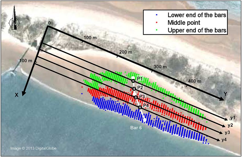
E. Pellón et al.: Intertidal finger bars at El Puntal, Bay of Santander, Spain                                                     351

migrate in the direction of sediment transport, but trans-
port direction is not always identified, possibly due to the
lack of field data. The theoretical modelling studies of Ribas
et al. (2003) and Garnier et al. (2006) have shown differ-
ent mechanisms to explain the dynamics of up- and down-
current-oriented bars by considering forcing due to waves.
Ribas et al. (2012) successfully applied their model to fin-
ger bars of an intermediate beach, based on continuous ob-
servations obtained from video imagery. However, the dy-
namics of finger bars appearing in low-energy environments
is poorly understood, especially concerning the small-scale
low-energy finger bars because (1) the forcing is difficult
to determine, with forces due to wind, waves and tidal cur-
rents all similar in magnitude in very limited fetch envi-
ronments, and (2) there has been no continuous, long-term
survey of such systems. Some observation studies on large-
scale finger bars have measured mean migration rates of less
than 2 m month−1 (Gelfenbaum and Brooks, 2003; Levoy
et al., 2013) and maximum speeds of 1 m day−1 (Levoy et al.,
2013). For the case of small-scale low-energy finger bars,
only the preliminary study of Garnier et al. (2012) has given
information on the dynamics of such systems, but the migra-
tion rates detected are overestimated due to strong noise in
the data.
   The objective of this contribution is to gain insight into the
dynamics of small-scale low-energy transverse bars by per-
forming a continuous survey of finger bars detected in the
Bay of Santander, Spain, and by analysing the possible forc-
ing mechanisms. These finger bars are located in the inter-
tidal zone, and the survey is performed by using video im-          Figure 1. (a) Location of Santander, (b) map of the bay, (c) El Pun-
ages at low tide. Section 2 presents the field site and the data    tal at high tide, and (d) El Puntal at low tide. Images from Google
                                                                    Earth; Landsat; © 2009 GeoBasis-DE/BKG; © 2013 Google; US
set obtained by video imagery. Section 3 describes the char-
                                                                    Dept of State Geographer; Data SIO, NOAA, U.S. Navy, NGA,
acteristics and the dynamics of the bar system. Section 4 re-       GEBCO; © 2013 DigitalGlobe.
ports the forcing analysis based essentially on wind data. The
conclusions are listed in Sect. 5.

2     Field site and video imagery
                                                                    (Losada et al., 1992; Kroon et al., 2007; Requejo et al., 2008;
2.1    Study site
                                                                    Medellín et al., 2008, 2009; Gutiérrez et al., 2011), but the
                                                                    lower-energy southern face remains unstudied. The incom-
El Puntal Spit is part of the natural closure of the Bay of San-    ing swell from the Cantabrian Sea only reaches the northern
tander (Fig. 1). This bay is one of the largest estuaries on the    face of the spit (Medellín et al., 2008). The southern pro-
northern coast of Spain (Cantabrian Sea). The closure of the        tected beaches of El Puntal are part of the bay and are located
bay is composed of two natural formations, the Magdalena            in a low-energy mesotidal environment. The maximum range
Peninsula to the north-west, and El Puntal Spit to the north-       of the semidiurnal tide is 5 m. Recent hydrodynamic studies
east. This spit is a sand accumulation which extends from           (Bidegain et al., 2013) have reported an ebb-oriented mean
east to west over approximately 2.5 km. Historically, more          annual flow of up to 0.1 m s−1 in the channel to the south of
than 50 % of the surface of this bay has been filled in, reduc-     El Puntal. This flow is mainly driven by the (ebb-dominated)
ing the tidal prism and changing the morphological equilib-         tidal current and by the flow from the Miera River, which en-
rium of El Puntal (Losada et al., 1991), which tends to extend      ters the bay at the east end of the El Puntal Spit. In the shal-
westward. However, for navigation purposes (Medina et al.,          lower areas the mean flow is much weaker and wind effects
2007), the entrance channel is periodically dredged, and thus       can become predominant (Bidegain et al., 2013), especially
the west end of El Puntal is maintained artificially.               if we take into account the waves that can be generated over
   There are numerous studies on El Puntal analysing the            a fetch of up to 4.5 km from the south-west direction. The
morphodynamics of the northern face and the west end                fetch is highly variable over a tidal cycle due to the numerous

www.earth-surf-dynam.net/2/349/2014/                                                      Earth Surf. Dynam., 2, 349–361, 2014
352 E. Pellón et al.: Intertidal finger bars at El Puntal, Bay of Santander, Spain
intertidal shoals in the bay (Fig. 1b), which can reduce the
maximum fetch to 200 m at low tide.
The finger bar system is located in the intertidal zone of
the beach on the southern side of the spit. Aerial images show
a system of 15 well-developed finger bars that is fully sub-
merged at high tide (Fig. 1c) and fully emerged at low tide
(Figs. 1d and 2a). At mid-tide the coastline exhibits a cuspate
shape (Fig. 2) and processes of wave refraction and wave
breaking are observed (Fig. 2c).
The alongshore extent of the bar system is less than 600 m
and the mean bar wavelength is about 25 m. The cross-shore
extent of the bars is controlled by the horizontal tidal excur-
sion and is larger in the middle of the domain (130 m) than on Figure 2. Photos at (a, b) low tide and with (c, d) rising tide. Pic-
the lateral sides (70 m). The bars are almost parallel and have tures taken from the east end of the study area (a, c), and from the
an oblique orientation with respect to the low-tide coastline. west end (b, d). Capture date: 25 February 2012.
The bar angle with respect to the low-tide shore normal is
about 25◦ toward the southeast (where 0◦ would correspond
to shore normal, transverse bars). However, the western end
of the system is more irregular, with slight changes in bar
orientation and bifurcations (Fig. 1d).
The intertidal beach where the bars appear is planar
with a constant slope of approximately 0.015. The offshore
boundary of the bars is delimited by a steep slope that ends in
the subtidal channel. Sediment sampling has shown the same
grain size on bars and troughs with D50 = 0.27 mm.
2.2 Video imagery and bar detection Figure 3. Horus video system. (a) Cameras on the roof of Hotel
Real. (b) Image taken by camera 2.
In the last few decades, video monitoring systems have been
increasingly used to study the shoreline around the world
(Holman et al., 1993). To obtain geometric data of the bar
system, the images of the Horus video imagery system were
used (Medina et al., 2007). This system is composed of The data processed by Garnier et al. (2012) have been re-
four cameras located on the roof of Hotel Real, 91 m a.s.l. analysed in order to correct an apparent periodic movement
and 1.5 km from the study area (Fig. 3a). The Horus sta- due to sun shadows in the bars. The amplitude of this periodic
tion was established in 2008 and takes images every 10 min. movement is of the order of the pixel resolution, and it has
In the present study only camera 2 was used (Fig. 3b). The been found that its period is related to the capture times. This
pixel resolution on the study area is variable on the along- apparent movement seems to be a systematic error linked to
shore direction, with values from 4.5 to 6.6 m pixel−1 . In the the different sun positions at low tide during the fortnightly
cross-shore direction the resolution is around 0.5 m pixel−1 . cycle of neap-spring tides, which causes different shadows
One daily image of the bar system has been selected at low due to the bars and different light reflections in the wet areas.
tide between 23 June 2008 and 2 June 2010, which is the This light shadowing/reflection also occurs for fixed struc-
longest period found without long interruptions in the image tures present in the surrounding areas. This allowed us to
database. All the interruptions were of less than 6 consecu- partially correct this spurious movement.
tive days and were due to technical problems (27 days) and For further analysis, a local, approximately shore-parallel
poor meteorological conditions (fog 18 days, strong wind coordinate system has been defined with the alongshore,
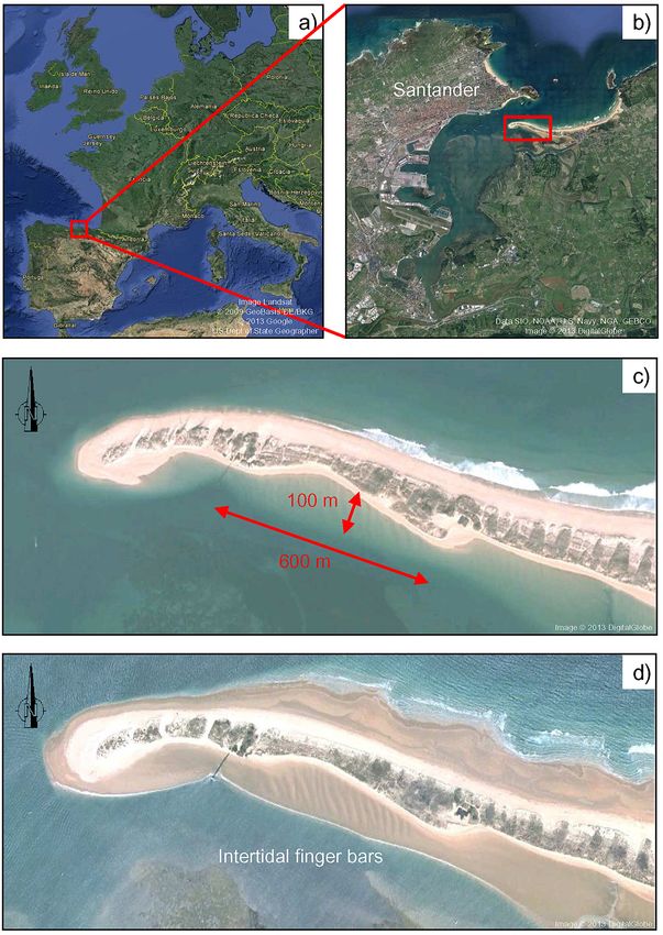
3 days and bad sharpness 85 days). The geometry of the bars y axis at 113◦ from north (Fig. 4). Within the new coordinate
was extracted on 577 days, which is 81 % of the time. system, the mean shoreline position now is approximately
Each bar has been digitised manually by selecting three parallel to the y axis during most of the tidal cycle. To bet-
points along the trough at the upper, middle and lowest end of ter understand the behaviour of the finger bars, the digitised
each bar (Fig. 4). Three points were found to describe the po- bars are then subsampled at x1 = 45, x2 = 65, x3 = 85, and
sition and orientation sufficiently. These digitised data were x4 = 105 m over the length of the alongshore domain (y1–
rectified using seven geographic control points (GCP), estab- y4 axes; see Fig. 4). These positions have been chosen to
lished for the Horus system, thus giving geographic coordi- give complete cross-shore coverage of the bars, and each one
nates of each digitised bar. is representative of one level of the beach profile (Fig. 5c).
Earth Surf. Dynam., 2, 349–361, 2014 www.earth-surf-dynam.net/2/349/2014/
E. Pellón et al.: Intertidal finger bars at El Puntal, Bay of Santander, Spain                                                     353

                                                                        (the segment k has a length of Tk ). For each segment, we
                                                                        can therefore obtain the approximate bar migration rate Vk ,
                                                                        which is the migration rate of this bar during the time interval
                                                                        Tk .
                                                                           Considering that, at a time t, N segments are obtained
                                                                        (where N is the number of bars of the system at this time
                                                                        t, multiplied by 4, which is the number of cross-shore posi-
                                                                        tions studied), the time-dependent migration rate of the bar
                                                                        system Vm (which is the average of the speeds, at this time t,
                                                                        of all the bars on all the cross-shore positions) is computed
                                                                        as
                                                                                                                  (
                                                                                  N (t)
                                                                                  X     V̂i (t)                    Vk , if t ∈ Tk
                                                                        Vm (t) =                , where V̂i (t) =                    (1)
                                                                                  i=1
                                                                                        N (t)                      0,   otherwise .
Figure 4. Coordinate system and bar digitisation. The x and y axes
stand for the cross-shore and the alongshore direction respectively.
The colour points represent the digitised data (each bar is repre-      3     Bar characteristics and dynamics
sented by three points); blue, red and green are the lowest, the mid-
dle and the upper points of the bars respectively. The bar positions    3.1    Bathymetry reconstruction
(P1–P4) are defined along the y1–y4 axes, at x1 = 45, x2 = 65,
x3 = 85, and x4 = 105 m respectively (see positions of bar 6, in        A bathymetry reconstruction has been done on 12 days with
white). Image from Google Earth, © 2013 DigitalGlobe.                   excellent meteorological conditions. Figure 5a shows the
                                                                        bathymetry obtained for 24 June 2008, the day with the
                                                                        best image quality. Cross-shore profiles of this bathymetry
2.3   3-D geometry                                                      (Fig. 5c) show that the bars only appear on the region of the
                                                                        intertidal beach profile which has constant slope of 0.015.
The Horus system captures one image of the study area every
                                                                        The extraction of alongshore profiles from these bathyme-
10 min. This means that the path of the shoreline can be ob-
                                                                        tries allows us to measure the amplitude of the bars, which
served along the tidal cycle with high frequency. To extract
                                                                        oscillates between 10 and 20 cm. These profiles also show the
information about the 3-D geometry of the finger bar system,
                                                                        asymmetry of the bars (Fig. 5b) with steeper slopes on the lee
a reconstruction of the intertidal bathymetry of the study area
                                                                        sides (relative to the migration direction), in agreement with
has been performed by mapping the shoreline from every im-
                                                                        previous studies (Gelfenbaum and Brooks, 2003).
age. This must be done on a day with perfect conditions, as
the meteorological conditions and image sharpness need to
be excellent. Furthermore, the tide should have the highest             3.2    Bar dynamics
range possible, allowing the extraction of a large intertidal           During the 2-year study period the position and geometry
region, and this must occur during daylight hours.                      of 15 bars were digitised daily. Figure 6 shows the posi-
   On good days, the shoreline is digitised and rectified on            tion of the bar system along the y3 axis once the digitised
each image. To obtain the bathymetry we assume that the sea             data have been corrected, rectified and transformed to the de-
level measured at the tide gauge of Santander (less than 2 km           scribed coordinate system (Fig. 4). Taking into account that
away) is the same as the level of the shoreline in the study            the pixel resolution on the study area is of about 5 m pixel−1
area. The tide level (with respect to the local Santander Har-          in the alongshore direction, the small oscillations visible in
bour datum, Z) at the time of each image is associated with             Fig. 6 are not deeply analysed, as they could be either phys-
the rectified shoreline from that image, obtaining an intertidal        ical or measurement errors. The bar system is persistent in
bathymetry.                                                             time, appearing in all the observed images with similar geo-
2.4   Piecewise regression of the bar movement
                                                                        metric characteristics, but the entire system slowly migrates
                                                                        to the east. As a result of the eastward migration a new bar
The method proposed here to find the time-dependent migra-              becomes visible at the western end of the study area (bar 1,
tion rates is based on piecewise regressions. This allows us            Fig. 6). Although aerial images and the migration of the sys-
to focus on the medium-term movements rather than on the                tem suggest that the bars are formed at the west of the study
daily fluctuations. The time series of the bar position for each        area, the formation area is not included in the present results
bar at each cross-shore position has been decomposed into               as it is hidden by the dune (Fig. 5a). At the eastern end of the
segments of variable length. The segment length has been set            area, the last bar decays and slowly disappears. In addition,
in order to minimise the error between the piecewise segment            during the study period, only one episode of merging of two
and the measured positions. After this decomposition, each              bars into one has been detected, on 28 March 2009 (bars 5–6,
bar is represented by several segments of different lengths             Fig. 6).

www.earth-surf-dynam.net/2/349/2014/                                                          Earth Surf. Dynam., 2, 349–361, 2014
354 E. Pellón et al.: Intertidal finger bars at El Puntal, Bay of Santander, Spain
Figure 6. Evolution of the bar system. Time series of the bar po-
sition along the y3 axis. The thin, discontinuous lines represent the
measured position. The thick segments represent the piecewise re-
gression of the measured position. The number to the left of each
line indicates the bar number.
Figure 5. (a) Bathymetry reconstruction with videoed shoreline po-
sitions during rising tide (24 June 2008). The north–west area with-
out data is the shadowed area by the dune, from the point of view of
the camera. (b) Alongshore profile of the bed level. (c) Cross-shore
profiles of the bed level and cross-shore positions of the y1–y4 axes.
Image from Google Earth, © 2013 DigitalGlobe.
3.2.1 Time-averaged characteristics
Figure 7. Time-averaged wavelength, angle and migration rate of
each bar. The bar angles are measured from the shore normal to the
The digitised and rectified data allow the daily measurement
east. Positive values of the bar speeds represent movements of the
of the bar wavelength. The bar wavelength is computed as the
bars to the east.
difference between the positions (on the yi axis) of two con-
secutive troughs. For each bar, the wavelength has been aver-
aged over the complete study period (Fig. 7). The wavelength
is approximately constant for each bar during the study pe-
riod (standard deviation, σ , around 4 m for all bars), but speed of each bar (for the whole study period) is shown in
varies between bars, with a minimum of 15 m and a maxi- Fig. 7. All the bars of the system slowly migrate to the east,
mum of 36 m. The mean wavelength of the whole bar system with a mean speed of 6 cm day−1 (approximately one wave-
is 25.8 m. length per year). The maximum migration rate is obtained
Similarly, the variability of the mean bar angle is low, with for the bar with the shortest wavelength (8 cm day−1 , bar 5)
σ around 5◦ for each bar. The mean angle of the system, that merges with the next bar, which is longer and slower
measured from the x axis, is 26.4◦ , with a maximum angle (bar 6). In general, the longer the wavelength, the slower the
of 34◦ at the western end, decreasing to a minimum of 17◦ at migration rate. This is in agreement with previous studies on
the eastern end (Fig. 7). The bars are not straight in plan view, transverse bars (Garnier et al., 2006).
so their angle has also been studied by splitting the bars into There are noticeable differences in the dynamics and in
two parts, the upper (onshore) half and the lower (offshore) the characteristics of the first five bars (western bars) com-
half. The upper part of all the bars has a lower angle with the pared with the eastern bars. The western bars (close to the
shore normal (mean of the whole system of 23◦ ), while the formation zone) are more irregular in shape, with a larger
lower part has higher angles (mean of 31◦ ). mean angle (5◦ larger), a smaller wavelength (20 m mean)
The time series of bar position is almost continuous and and a corresponding higher migration rate. The eastern bars
allows us to compute the time-averaged migration rate of the are well defined and remarkably parallel. Their cross-shore
system, which is obtained by linear regression. The mean span decreases as they approach the decaying zone.
Earth Surf. Dynam., 2, 349–361, 2014 www.earth-surf-dynam.net/2/349/2014/E. Pellón et al.: Intertidal finger bars at El Puntal, Bay of Santander, Spain 355 3.2.2 Time-dependent migration rates Each bar signal has been decomposed into 10 segments by means of the piecewise regression described in Sect. 2.4 (Fig. 6). It was found that 10 is the best number to repre- sent the medium-term movement of the bar and to filter the daily fluctuations. As we are analysing 2 years of data, the mean segment length is 70 days. The migration rate of the bar system Vm , computed with (Eq. 1), is not constant in time with maximum migration rates in winter (Fig. 8). The maximum speeds, about 0.15 m day−1 , are reached during the first winter studied (2009), while dur- ing the second winter (2010) the maximum speeds are lower than 0.1 m day−1 . During summer the system migration is slower, with negative speeds for summer 2008, and migration rates lower than 0.01 m day−1 for summer 2009. The nega- tive speeds (i.e. migration to the west) found in summer 2008 Figure 8. Vm (thick black line), time-dependent migration rate of can be due to limitations in the computation of Vm . Specif- the entire bar system (average of all coloured lines). Vk (colour ically, the accuracy of the piecewise regression is expected lines), individual bar migration rate (the colours correspond to to be lower at the beginning and end of the time series, due Fig. 6). (a) Vk for bars 3–8. (b) Vk for bars 9–14. to the lack of previous/subsequent data. The negative migra- tion rate is obtained for the first segment of the bars only; therefore this result may not be realistic. 4 Forcing analysis 4.1 Forcing candidates The migration to the east of the bar system indicates a domi- nant forcing coming from the west. The wind data have been extracted from the SeaWind (Menéndez et al., 2011) reanal- ysis database. Figure 9a shows the wind rose, and the time series of the wind speed is displayed in Fig. 9c. The pre- dominant wind is from the west, reaching values of up to 25 m s−1 . The wind from the east is also frequent but less energetic, with speeds lower than 15 m s−1 . The mean wind speed is 5 m s−1 . Other studies on transverse bars (Ribas et al., 2003) sug- gest that waves are the main forcing that controls their dy- namics. The study area is protected from the incoming swell (Medellín et al., 2008) and the waves that can act on the bar system are generated locally. According to estuarine studies these wind waves can have a significant effect in the sediment transport (Green et al., 1997). Here, wind waves are gener- ated over a maximum fetch of 4.5 km (from the south-west of the study area). Toward the south and south-east the fetch is reduced by the proximity of land. During the survey period, the tidal range oscillates be- tween 1 and 5 m (Fig. 9d). Maximum values of the tidal cur- rent in the channel (offshore of the bar system) occur during spring tides, with values of up to 0.25 m s−1 . In the chan- nel the mean (residual) flow is ebb-oriented, but the resid- Figure 9. (a) Wind rose. (b) Wave rose. (c–f) Time series of ual tidal current is small in the intertidal areas. Computations the (c) wind speed W , and the daily averaged (d) tidal range, performed (not shown) with an H2D model (Bárcena et al., (e) river flow rate and (f) root-mean-squared wave height of the 2012) show that the maximum residual current (obtained dur- wind waves Hrms . www.earth-surf-dynam.net/2/349/2014/ Earth Surf. Dynam., 2, 349–361, 2014
356                                                E. Pellón et al.: Intertidal finger bars at El Puntal, Bay of Santander, Spain

ing spring tides) is lower than 0.01 m s−1 in the study area.      energy flux (e.g. Castelle et al., 2007; Price and Ruessink,
Although the residual current is small, the tide can have an       2011) or the wave radiation stress (e.g. Ribas and Kroon,
effect on the bar dynamics because tidal currents can cause        2007).
sediment stirring (which is stronger during mid tides) and           Here, the effect of the local wind is also analysed by com-
because of the changes in water level. Firstly, the fetch is       puting the alongshore component of the wind shear stress
strongly dependent on the water level (Green et al., 1997)         acting on the water surface (Figs. 10a and 11a), defined as
according to the emersion and submersion of the numerous           (Dean and Dalrymple, 1991)
intertidal shoals during the tidal cycle, and this is taken into
account in the wave computations (see Sect. 4.2.1). Secondly,      Ty = −ρCf W 2 cos θw ,                                       (2)
the changes in tidal level affect the time of bar submersion
(that is larger during neap tides) and the volume of sand that     where ρ is the water density (ρ = 1025 kg m−3 ); Cf is the
can be transported (larger if high tide coincides with strong      friction coefficient, equal to 1.2×10⁻⁶ ; W is the wind speed;
winds/waves). This will be taken into account in the sediment      and θw is the incoming wind angle (from the shore normal).
transport computations by including the tidal correction fac-         In order to compare the relative effect of the wind stress
tor (see further explanations in Sect. 4.3.2).                     and of the wave radiation stress, we define the alongshore
   Hydrodynamic studies of the Santander Bay have high-            wave stress, Sy = Sxy /Xb (Figs. 10b and 11b). Sxy is the
lighted the effect of the water discharge produced by the          alongshore component of the wave radiation stress (Longuet-
Miera River (to the east of the study area) in the annual mean     Higgins and Stewart, 1964) and Xb is the surf-zone width. By
current magnitude in the bay (Bidegain et al., 2013). Time se-     considering Xb = Hrms /(β γb ), we obtain
ries of the daily averaged river flow rate are shown in Fig. 9e.
                                                                          ρg Hrms
Bidegain et al. (2013) have shown that, although the effect        Sy =           sin θ cos θ,                                  (3)
of the river is strong in the channel (ebb-oriented flow), the            16 βγb
current produced close to the bar system is weak. However,
                                                                   where g is the gravitational acceleration (g = 9.81 m s−2 ),
the river discharge can play a role in the bar dynamics as it is
                                                                   γb is the breaking coefficient for irregular waves (γb = 0.42,
linked to a strong sediment supply, which can act as an input
                                                                   Thornton and Guza, 1983), β is the beach slope (β = 0.015)
of suspended sediment to the bar system.
                                                                   and θ is the offshore wave angle (from the shore normal). Sy
                                                                   is an approximation of the term ∂Sxy /∂y in the alongshore
4.2     Wind acting on water surface                               momentum balance equation, a term that is equivalent to Ty
4.2.1    Wave computation                                          in the same equation.
                                                                      Figure 11a and b show the seasonal variability of Sy and Ty
The wind waves over the system have been simulated from            respectively. The comparison of both figures shows that both
the wind speed and direction by using the SWAN model               forcings are of the same order of magnitude and can there-
(Booij et al., 1999). In the computations, changes in tidal        fore play a role in the bar dynamics, although Sy is twice
level affecting the fetch have been included. The time series      as large as Ty . Only the wind stress seasonal analysis shows
of the wind waves has been obtained with an interpolation          more highly energetic conditions in winter 2009 than in win-
technique based on radial basis functions (RBF), a scheme          ter 2010, in accordance with the results of the migration rate.
which is convenient for scattered and multivariate data (Ca-       However, the wind stress shows more highly energetic con-
mus et al., 2011). Results of the root-mean-squared (rms)          ditions in autumn than in winter, while the migration rate
wave height Hrms of the waves approaching the bar system           shows lower values in autumn 2009 than in winter 2009.
are displayed in Fig. 9b (wave rose) and in Fig. 9f (time          The wave stress seasonal analysis shows lower differences
series of the daily averaged Hrms ). The waves arrive from         between autumns and winters, with larger values still being
the west-south-west and south-west 65 % of the time, with a        in the autumn.
mean Hrms of 5 cm and a period of 1.5 s. During the westward
windstorms the waves can extend to 20 cm from the west-
south-west, with a period of 3 s. The other 35 % of the time       4.3    Sediment transport
the waves come from the east-south-east, with Hrms lower
                                                                   The relationship between the bar migration and the along-
than 7 cm and periods below 1.7 s. The mean Hrms from this
                                                                   shore component of the sediment transport is also investi-
sector is less than 2 cm with a period of 1.2 s.
                                                                   gated. We use a formulation based on the Soulsby and Van
                                                                   Rijn formula (Soulsby, 1997). This formulation has been
4.2.2    Wind stress vs wind-wave stress forcing                   used in modelling studies to explain the formation of differ-
The previous studies on transverse bars, where the waves ap-       ent kinds of transverse bars (Ribas et al., 2012; Garnier et al.,
pear to be the main forcing, usually focus on wave parame-         2006).
ters to relate the dynamics of the bars with the incident wave
forcing, for example the alongshore component of the wave

Earth Surf. Dynam., 2, 349–361, 2014                                                   www.earth-surf-dynam.net/2/349/2014/
E. Pellón et al.: Intertidal finger bars at El Puntal, Bay of Santander, Spain 357
Figure 10. Time series of the daily averaged (a) alongshore wind
stress (Ty , black) and (b) alongshore wave stress (Sy , black). The
grey lines represent the behaviour of the bar migration rate Vm that
has been rescaled with the above variables.
4.3.1 Soulsby and Van Rijn formula
Here, we assume that the general formulation of the along- Figure 11. Seasonal variability of (a) alongshore wind stress (Ty )
shore component of the sediment transport is given by and (b) alongshore wave stress (Sy ). The black lines represent the
behaviour of the bar migration rate Vm that has been rescaled with
q = α (Vwave + Vwind ) , (4) the above variables. The bottom axes indicate the seasons, from
summer 2008 to spring 2010.
where α is the sediment stirring function, Vwave is the along-
shore component of the wave- and depth-averaged current
driven by the wind waves, and Vwind is the alongshore com- above which the sediment can be transported. AS and Ucrit
ponent of the depth-averaged current driven by the local depend essentially on the sediment characteristics and on
wind. the water depth (for more details see Soulsby, 1997; Garnier
The alongshore current generated by the wind waves is ap- et al., 2006). The equivalent stirring velocity is defined as
proximated from the formula presented by Komar and Inman
0.018 2 0.5
(1970): 2 2
Ueq = Uwind + Vwave + Ub , (8)
0.5 Cd
Vwave = 1.17 (gHrms ) sin θb cos θb , (5)
where Ub is the wave orbital velocity amplitude at the bottom
where θb is the wave angle at breaking. By using Snell’s law (computed at wave breaking), Cd is the morphodynamic drag
and the dispersion relationship, Eq. (5) has been evaluated at coefficient computed with the formula of Soulsby (1997) and
the breaking depth, defined as Hrms /γb (γb = 0.42) from Uwind is the modulus of the current generated by the wind:
the incident wave angle computed with the SWAN model
(Sect. 4.1).
Cf 2
0.5
The alongshore current generated by the wind is computed Uwind = W . (9)
cd
by assuming the alongshore momentum balance between the
wind stress and the bottom friction in the case of a quadratic
friction law: 4.3.2 Tidal correction factor
Ty 0.5 Although the tidal level variations have been included to
Vwind = ± , (6) compute the incoming wave time series, the sediment trans-
ρcd port formula defined in Sect. 4.3.1 does not take into account
where cd is the hydrodynamic drag coefficient set as cd = that the bars can be emerged, and are therefore inactive, dur-
0.005. ing part of a tidal cycle. If strong winds and high waves (de-
The stirring function in Eq. (4) is approximated with the spite the limited fetch) coincide with the time of emersion,
Soulsby and Van Rijn formula (Soulsby, 1997) as they will have no effect and the effective sediment transport
( 2.4 should be zero. Furthermore, the time of submersion depends
AS Ueq − Ucrit if Ueq > Ucrit on the tidal range. During neap tides the bar system is af-
α= (7) fected by the marine dynamics almost 100 % of the time be-
0 otherwise ,
cause the full emersion of the bars occurs only when the tide
where AS is a coefficient that represents the suspended load is at its lowest level (during a short time period). However,
and the bed load transport and Ucrit is the critical velocity during spring tides, the active time period is reduced because
www.earth-surf-dynam.net/2/349/2014/ Earth Surf. Dynam., 2, 349–361, 2014358 E. Pellón et al.: Intertidal finger bars at El Puntal, Bay of Santander, Spain
the tide falls lower and the bars stay emerged for a longer
time.
These effects have been quantified by means of a tidal cor-
rection factor (αt ), ranging from 0 to 1, which evaluates how
exposed the bars are due to the stirring resulting from the hy-
drodynamics. The corrected transport formula is then com-
puted as
q t = αt q; (10)
Figure 12. Parameters for the calculation of the tidal correction
αt varies every hour, depending on the surf-zone width (Xb ) factor (αt ), which depends on the tidal level (ηt ); the mean cross-
shore span of the bars (L); the active depth (h∗ ); the surf-zone width
and on the tidal level (ηt ). It is computed by using the follow-
(Xb ); and the level of the bar lower end (Z0 ), the bar upper end (Z2 )
ing formula (see Fig. 12):
and the levels Z1 and Z3 , which vary with the wave height (Hrms ).
0 if Z3 < ηt
Z3 − ηt
α if Z2 < ηt < Z3
Z3 − Z2 t,max
αt = αt,max if Z1 < ηt < Z2 (11)
η − Z
t 0
αt,max if Z0 < ηt < Z1
Z 1 − Z 0
0 if ηt < Z0 , Figure 13. Time series of: the tidal correction factor αt (red dots);
and the tidal range (greyscale, vertical bars).
where αt,max quantifies the ratio between the surf-zone width
(corresponding to the Hrms ) and the cross-shore span of the
bars, representing the percentage of the bars that could be From our observations, the tidal factor never reaches 1
within the active surf zone, (Fig. 13). αt = 1 could occur for strong stormy conditions
if the surf-zone width is as large as the bar width L (Hrms >
Xb Hrms 0.5), and if it coincides with high tide (ηt = Z2 ). Figure 13
αt,max = = , (12)
L βγb L shows that αt reaches its maximum values during neap tides,
as was expected, generally as the tidal level is close to Z2 a
where L is the mean cross-shore span of the bars (L =
larger part of the day. During spring tides, the time during
100 m) and Xb is the width of the active surf zone (Fig. 12).
which the tidal level is between Z3 and Z0 is highly reduced.
Z0 , Z1 , Z2 and Z3 are defined as (see Fig. 12)
Consequently, the tidal factor is generally minimum.
Z0 = 2.5 m = level of the bar lower end
4.3.3 Results
Z1 (t) = Z0 + h∗ (t) = 2.5 + γ −1 Hrms (t)
b
(13) In order to analyse the correlation between q and the bar mi-
Z 2 = 3.7 m = level of the bar upper end gration rate Vm , the time-dependent sediment transport rate
Z3 (t) = Z2 + h∗ (t) = 3.7 + γb−1 Hrms (t). must be computed. First, we integrate the sediment trans-
port over the time intervals Tk , for each segment that char-
Z0 and Z2 (levels of the bar lower end and upper end) are acterises the bar movement (as explained in Sect. 3.2.2), and
constant and determined from the 3-D-geometry (Fig. 5). then we apply an equation equivalent to Eq. (1) for that sed-
Z1 and Z3 depend on the active depth h∗ defined as (h∗ = iment transport data. The obtained time series of the time-
Hrms /γb ). dependent sediment transport is shown in Fig. 14.
To better understand these formulas, let us consider a day Figure 14a, which displays the sediment transport with-
with constant wave height. The tidal correction factor is ma- out the tidal correction, shows that the sediment transport is
ximum (αt = αt,max ) when the maximum depth at the bars is weaker in spring 2009 than in spring 2010, corresponding to
larger than the active depth (ηt ≥ Z1 ) and when the sea level a smaller migration rate. However, the seasonal average of q
does not exceed the upper end of the bars (ηt ≤ Z2 ). This shows similar values for autumn–winter 2009 and autumn–
means that the complete surf-zone width is located over the winter 2010, while the migration rate results show lower
bars. Furthermore, the sediment transport over the bars van- values during 2010. The correlation coefficient obtained is
ishes if the sea level does not reach the lower end of the bars r = 0.75.
(ηt ≤ Z0 , i.e. too shallow) and if the minimum water depth The addition of the tidal factor improves the results
at the bars is larger than the active depth (ηt ≥ Z3 , i.e. too (Fig. 14b) increasing the correlation coefficient to r = 0.8.
deep). All correlations obtained are highly significant (p < 0.001).
Earth Surf. Dynam., 2, 349–361, 2014 www.earth-surf-dynam.net/2/349/2014/E. Pellón et al.: Intertidal finger bars at El Puntal, Bay of Santander, Spain 359
5 Conclusions
A small-scale finger bar system has been identified on the in-
tertidal zone of the swell-protected beach of El Puntal Spit
in the Bay of Santander (northern coast of Spain). The beach
is characterised by a constant slope of 0.015 and by uniform
sand with D50 = 0.27 mm. This system appears on the flat in-
tertidal region, which extends over 600 m on the alongshore
direction and between 70 and 130 m on the cross-shore di-
rection (the cross-shore span is determined by the tidal hori-
zontal excursion).
A system of 15 bars was observed by using the Horus
video imaging system during 2 years (between 23 June 2008
and 2 June 2010). The bar system has been digitised from
daily images at low tide. The data set is almost continuous,
with good quality data 81 % of the time and a maximum con-
tinuous period of time without data of no more than 6 days.
The geometric characteristics of the system are almost
Figure 14. Sediment transport evaluation. Analysis of (a) along- constant in time. The mean wavelength of the bar system is
shore component of sediment transport q (without tidal correction), 26 m and the bar amplitude is between 10 and 20 cm. More-
and (b) q t (with tidal correction). The grey areas show the season- over, the bars have an oblique orientation with respect to the
ally averaged transport and the red lines show the time-dependent low-tide shoreline, with a mean angle of 26◦ to the east from
sediment transport time series (obtained by averaging over the Tk the shore normal. We noticed differences in the geometry
intervals). The black lines represent the behaviour of the bar migra- along the domain: the western bars (first half) are more ir-
tion rate Vm that has been rescaled with the above variables. The
regular and have smaller wavelength than the eastern bars
correlation coefficient of both lines is shown in the bottom right
(second half).
corner. The bottom axes indicate the seasons, from summer 2008 to
spring 2010. The full system slowly migrates to the east (against the ebb
flow) with a mean speed of 6 cm day−1 that varies between
bars. In general, larger wavelength bars migrate more slowly,
The seasonal analysis shows higher values of sediment trans- in agreement with previous studies (Garnier et al., 2006).
port during autumn–winter 2009 than autumn–winter 2010, An episode of merging of two bars was observed on 28
corresponding with higher time-dependent migration rates March 2009: the bar with the smallest wavelength is faster
during autumn–winter 2009. Again, the sediment transport and merges with the next bar. Bars form on the western end
computed in spring 2009 is lower than in spring 2010, cor- of the system, migrate east and then decay at the eastern end.
responding well with the smaller migration rates measured A detailed analysis of the bar motion, from a piecewise
in spring 2009. The time-dependent sediment transport time regression of the bar positions, has shown that bars migrate
series of q t (Fig. 14b) follows the main shape of the mea- more quickly in winter than in summer, with maximum mi-
sured time-dependent migration rate. The bigger differences gration rates obtained in winter 2009 (0.15 m day−1 ). Some
are found at the beginning and end of the study period, where negative speeds (migration to the west) have been computed
the time-dependent migration rates are less reliable, as ex- (during summer 2008), but this result could be an effect of
plained in Sect. 3.2.2. In particular, none of the formulas the limitations of the piecewise regression at the beginning
used managed to predict the negative (westward) migration and end of the time series.
reported during summer 2008, but, as previously mentioned, The primary forcing mechanism that is acting on the bar
these negative migration rates may be not realistic. dynamics is the wind over the water surface. Offshore of
Figure 9e shows the flow rate of Miera River. This flow the bar system, the mean (annual) flow is ebb-oriented (to
rate is greater during winter 2009 than winter 2010, so the the west), because of the Miera River discharge and the as-
faster migration rate of the bars during this period could tronomical tide. However, in the intertidal zone their effects
be influenced by the river discharge, possibly because it is on the mean flow vanish. There, wind shear stress and wind
a source of sediment. However, tests performed by including waves generated over a fetch of up to 4.5 km at high tide
additional sediment stirring due to the river flow do not show seem to determine the direction of the alongshore transport.
improvement in the results. Although the residual tidal current is weak, the tide seems
to be important in the bar dynamics as the tidal range changes
the mean (daily) fetch as well as the time of exposure of the
bars to the marine dynamics. Furthermore, the river discharge
www.earth-surf-dynam.net/2/349/2014/ Earth Surf. Dynam., 2, 349–361, 2014360 E. Pellón et al.: Intertidal finger bars at El Puntal, Bay of Santander, Spain
could act as input of suspended sediment in the bar system Castelle, B., Bonneton, P., Dupuis, H., and Senechal, N.: Double
and play a role in the bar dynamics. bar beach dynamics on the high-energy meso-macrotidal French
The correlation between the bar migration and the along- Aquitanian coast: a review, Mar. Geol., 245, 141–159, 2007.
shore component of the sediment transport has been anal- Dean, R. G. and Dalrymple, R. A.: Water wave mechanics for engi-
ysed by using the Soulsby and Van Rijn formulation. The in- neers and scientists, World Scientific, 157–158, 1991.
Falqués, A.: Formación de topografía rítmica en el Delta del Ebro,
clusion of a tidal correction factor, simulating that the active
Revista de Geofísica, 45, 143–156, 1989 (in Spanish).
time depends on the tidal level and the wave height, improves Galal, E. M. and Takewaka, S.: Longshore migration of shoreline
the results. mega-cusps observed with x-band radar, Coast. Eng. J., 50, 247–
Finally, the bar system is persistent and neither formation 276, 2008.
nor destruction events of the entire system have been ob- Garnier, R., Calvete, D., Falqués, A., and Caballeria, M.: Gener-
served. Further studies are necessary to understand the for- ation and nonlinear evolution of shore-oblique/transverse sand
mation processes and the full dynamics of these small-scale bars, J. Fluid Mech., 567, 327–360, 2006.
finger bars. In situ measurements of the hydrodynamics and Garnier, R., Calvete, D., Falqués, A., and Dodd, N.: Modelling the
sediment concentrations, as well as numerical morpholog- formation and the long-term behavior of rip channel systems
ical modelling, are essential in order to deepen our under- from the deformation of a longshore bar, J. Geophys. Res., 113,
standing. The bar system here has an oblique down-current C07053, doi:10.1029/2007JC004632, 2008.
Garnier, R., Medina, R., Pellón, E., Falqués, A., and Turki, I.: Inter-
orientation with respect to the migration direction and has
tidal finger bars at El Puntal spit, bay of Santander, Spain, in: Pro-
similar characteristics and dynamics to the system described ceedings of the 33rd Conference on Coastal Engineering, ASCE,
by previous theoretical (modelling) studies that consider the Santander, Spain, 1–8, 2012.
forcing due to waves only (e.g. Garnier et al., 2006). How- Gelfenbaum, G. and Brooks, G. R.: The morphology and migration
ever, in our estuarine environment, the dynamics are more of transverse bars off the west-central Florida coast, Mar. Geol.,
complex as the actions of different forcings are of the same 200, 273–289, 2003.
order of magnitude. Goodfellow, B. W. and Stephenson, W. J.: Beach morphodynamics
in a strong-wind bay: a low-energy environment?, Mar. Geol.,
214, 101–116, 2005.
Green, M. O., Black, K. P., and Amos, C. L.: Control of estuarine
Acknowledgements. The authors thank Puertos del Estado sediment dynamics by interactions between currents and waves
(Spanish Government) for providing tide-gauge data. The work at several scales, Mar. Geol., 144, 97–116, 1997.
of R. Garnier is supported by the Spanish Government through Gutiérrez, O., González, M., and Medina, R.: A methodology to
the “Juan de la Cierva” programme. This research is part of the study beach morphodynamics based on self-organizing maps and
ANIMO (BIA2012-36822) project, which is funded by the Spanish digital images, in: Proceedings of the Coastal Sediments 2011,
Government. The authors thank the editor, G. Coco, and the World Scientific, 2453–2464, 2011.
referees, F. Ribas and E. Gallagher, for their useful comments. Holman, R. A., Sallenger Jr., A. H., Lippmann, T. C. D., and Haines,
J. W.: The application of video image processing to the study of
Edited by: G. Coco nearshore processes, Oceanography, 6, 78–85, 1993.
Komar, P. and Inman, D.: Longshore sand transport on beaches,
J. Geophys. Res., 75, 5514–5527, 1970.
Konicki, K. M. and Holman, R. A.: The statistics and kinematics of
References transverse sand bars on an open coast, Mar. Geol., 169, 69–101,
2000.
Bárcena, J. F., García, A., García, J., Álvarez, C., and Revilla, J. A.: Kroon, A., Davidson, M. A., Aarninkhof, S. G. J., Archetti, R., Ar-
Surface analysis of free surface and velocity to changes in river maroli, C., González, M., Medri, S., Osorio, A., Aagaard, T.,
flow and tidal amplitude on a shallow mesotidal estuary: an appli- Holman, R. A., and Spanhoff, R.: Application of remote sensing
cation in Suances Estuary (Nothern Spain), J. Hydrol., 14, 301– video systems to coastline management problems, Coast. Eng.,
318, 2012. 54, 493–505, 2007.
Bidegain, G., Bárcena, J. F., García, A., and Juanes, J. A.: LAR- Lafon, V., Dupuis, H., Howa, H., and Froidefond, J. M.: Determin-
VAHS: predicting clam larval dispersal and recruitment using ing ridge and runnel longshore migration rate using spot imagery,
habitat suitability-based particle tracking mode, Ecol. Model., Oceanol. Acta, 25, 149–158, 2002.
268, 78–92, 2013. Levoy, F., Anthony, E. J., Monfort, O., Robin, N., and Bretel, P.:
Booij, N., Ris, R. C., and Holthuijsen, L. H.: A third-generation Formation and migration of transverse bars along a tidal sandy
wave model for coastal regions, Part I, Model description and coast deduced from multi-temporal Lidar datasets, Mar. Geol.,
validation, J. Geophys. Res., 104, 7649–7666, 1999. 342, 39–52, 2013.
Bruner, K. R. and Smosna, R. A.: The movement and stabilization Longuet-Higgins, M. S. and Stewart, R. W.: Radiation stresses in
of beach sand on transverse bars, Assateague Island, Virginia, water waves: a physical discussion with applications, Deep-Sea
J. Coastal Res., 5, 593–601, 1989. Res., 11, 529–562, 1964.
Camus, P., Méndez, F. J., and Medina, R.: A hybrid efficient method
to downscale wave climate to coastal areas, Coast. Eng., 58, 851–
862, 2011.
Earth Surf. Dynam., 2, 349–361, 2014 www.earth-surf-dynam.net/2/349/2014/E. Pellón et al.: Intertidal finger bars at El Puntal, Bay of Santander, Spain 361 Losada, M. A., Medina, R., Vidal, C., and Roldan, A.: Historical Requejo, S., Medina, R., and González, M.: Development of evolution and morphological analysis of “EI Puntal” Spit, San- a medium-long term beach evolution model, Coast. Eng., 55, tander (Spain), J. Coastal Res., 7, 711–722, 1991. 1074–1088, 2008. Losada, M. A., Medina, R., Vidal, C., and Losada, I. J.: Tempo- Ribas, F. and Kroon, A.: Characteristics and dynamics of sur- ral and spatial cross-shore distributions of sediment at “El Pun- fzone transverse finger bars, J. Geophys. Res., 112, F03028, tal” spit, Santander, Spain, Coast. Eng., 1992, Proceedings of the doi:10.1029/2006JF000685, 2007. Twenty-Third International Conference, 2251–2264, 1992. Ribas, F., Falqués, A., and Montoto, A.: Nearshore Medellín, G., Medina, R., Falqués, A., and González, M.: Coastline oblique sand bars, J. Geophys. Res., 108, C43119, sand waves on a low-energy beach at “El Puntal” spit, Spain, doi:10.1029/2001JC000985, 2003. Mar. Geol., 250, 143–156, 2008. Ribas, F., de Swart, H. E., Calvete, D., and Falqués, A.: Model- Medellín, G., Falqués, A., Medina, R., and González, M.: Coast- ing and analyzing observed transverse sand bars in the surf zone, line sand waves on a low-energy beach at El Puntal spit, J. Geophys. Res., 117, F02013, doi:10.1029/2011JF002158, Spain: linear stability analysis, J. Geophys. Res., 114, C03022, 2012. doi:10.1029/2007JC004426, 2009. Ribas, F., ten Doeschate, A., de Swart, H., Ruessink, G., and Medina, R., Marino-Tapia, I., Osorio, A., Davidson, M., and Martín, Calvete, D.: Observations and modelling of surf-zone trans- F. L.: Management of dynamic navigational channels using video verse finger bars at the Gold Coast, Australia, Ocean Dynam., techniques, Coast. Eng., 54, 523–537, 2007. doi:10.1007/s10236-014-0719-4, in press, 2014. Menéndez, M., Tomás, A., Camus, P., García-Díez, M., Fita, L., Soulsby, R. L.: Dynamics of Marine Sands, Thomas Telford, Lon- Fernández, J., Méndez, F. J., and Losada, I. J.: A methodol- don, UK, 1997. ogy to evaluate regional-scale offshore wind energy resources, Thornton, B. and Guza, R. T.: Transformation of wave height dis- OCEANS’11 IEEE Santander Conference, Spain, 1–9, 2011. tribution, J. Geophys. Res., 88, 5925–5938, 1983. Niedoroda, A. W. and Tanner, W. F.: Preliminary study of transverse Thornton, E. B., MacMahan, J., and Sallenger Jr., A. H.: Rip cur- bars, Mar. Geol., 9, 41–62, 1970. rents, mega-cusps, and eroding dunes, Mar. Geol., 240, 151–167, Nordstrom, K. F. and Jackson, N. L.: Physical processes and land- 2007. forms on beaches in short fetch environments in estuaries, small van Enckevort, I. M. J., Ruessink, B. G., Coco, G., Suzuki, K., lakes and reservoirs: a review, Earth-Sci. Rev., 111, 232–247, Turner, I. L., Plant, N. G., and Holman, R. A.: Observations of 2012. nearshore crescentic sandbars, J. Geophys. Res., 109, C06028, Price, T. D. and Ruessink, B. G.: State dynamics of a double sandbar doi:10.1029/2003JC002214, 2004. system, Cont. Shelf. Res., 31, 659–674, 2011. Wijnberg, K. M. and Kroon, A.: Barred beaches, Geomorphology, Ranasinghe, R., Symonds, G., Black, K., and Holman, R.: Morpho- 48, 103–120, 2002. dynamics of intermediate beaches: a video imaging and numeri- Wright, L. D. and Short, A. D.: Morphodynamic variability of surf cal modelling study, Coast. Eng., 51, 629–655, 2004. zones and beaches: a synthesis, Mar. Geol., 56, 93–118, 1984. www.earth-surf-dynam.net/2/349/2014/ Earth Surf. Dynam., 2, 349–361, 2014
You can also read