Investigation of Hexavalent Chromium Flux to Groundwater at the 100-C-7:1 Excavation Site
←
→
Page content transcription
If your browser does not render page correctly, please read the page content below
PNNL-21845
                                             RPT-DVZ-AFRI-005

Prepared for the U.S. Department of Energy
under Contract DE-AC05-76RL01830

Investigation of Hexavalent
Chromium Flux to Groundwater at
the 100-C-7:1 Excavation Site

MJ Truex
VR Vermeul
BG Fritz
RD Mackley
JA Horner
CD Johnson
DR Newcomer

November 2012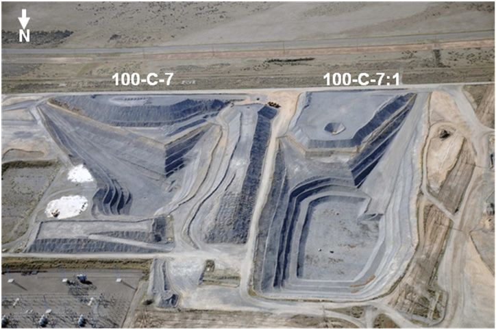
PNNL-21845
                                        RPT-DVZ-AFRI-005

Investigation of Hexavalent
Chromium Flux to Groundwater at
the 100-C-7:1 Excavation Site

MJ Truex
VR Vermeul
BG Fritz
RD Mackley
JA Horner
CD Johnson
DR Newcomer

November 2012

Prepared for
the U.S. Department of Energy
under Contract DE-AC05-76RL01830

Pacific Northwest National Laboratory
Richland, Washington 99352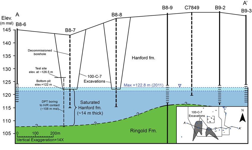
Executive Summary

     Deep excavation of soil has been conducted at the 100-C-7 and 100-C-7:1 waste sites within the
100-BC Operable Unit at the U.S. Department of Energy’s Hanford Site to remove hexavalent chromium
(Cr(VI)) contamination, with excavations reaching to near the water table. Soil sampling showed that
Cr(VI) contamination was still present at the bottom of the 100-C-7:1 excavation. In addition, Cr(VI)
concentrations in a downgradient monitoring well have shown a transient spike of increased Cr(VI)
concentration following initiation of excavation activities. Potentially, the increased Cr(VI) concen-
trations in the downgradient monitoring well are due to Cr(VI) from the excavation site. However, data
were needed to evaluate this possibility and to quantify the overall impact of the 100-C-7:1 excavation
site on groundwater. Data collected from a network of aquifer tubes installed across the floor of the
100-C-7:1 excavation and from temporary small-diameter wells installed at the bottom of the entrance
ramp to the excavation were used to evaluate Cr(VI) releases into the aquifer and estimate local-scale
hydraulic properties and groundwater flow velocity.

    The Cr(VI) data collected from project-installed aquifer tubes show a short-lived and relatively small
pulse of Cr(VI) was released to groundwater at the excavation site during the study period. This release
occurred in response to the seasonal rise in the water table, and associated saturation of excavation-
bottom sediments, resulting from an increase in Columbia River stage. By the end of the study period,
although the water table was still high, Cr(VI) concentrations had dissipated with no significant
continuing source observed, providing direct evidence that sorption of Cr(VI) to vadose zone or aquifer
sediments is minimal and that Cr(VI) present in the lower vadose zone is readily mobilized when the
sediments become saturated.

     Previously available hydraulic property information was sparse for the Hanford formation in the
100-BC Area. Taking advantage of the excavation depth, temporary small-diameter wells were installed
using economical direct-push methods. Hydraulic property information was determined by analysis of
constant rate injection hydraulic response data, tracer injection arrival curves, tracer elution response
under natural gradient conditions, and electromagnetic borehole flow meter data. Direct-push penetration
data also provided information about the local geological contact between the Hanford and Ringold
Formations. Based on the hydraulic/tracer testing data and associated local-scale estimates of
groundwater velocity in the vicinity of the 100-C-7:1 site, it is possible that Cr(VI) mobilized from the
excavation and released to groundwater between November 2011 and February 2012 could have resulted
in the Cr(VI) concentration peak observed in downgradient monitoring well 199-B4-14.

     Access to the excavation floor near the water table enabled collection of a large amount of hydrologic
and contaminant transport and distribution information within a short time frame. These data would be
costly and more difficult to obtain with wells installed from the ground surface. Other opportunities
where excavations provide relatively shallow access to the groundwater and enable use of direct-push
drilling could be used to augment the hydraulic and contaminant data for the Hanford Site. Importantly,
the ability to install multiple temporary wells enables use of constant rate injection (or discharge) testing
with a stressed well and observation well(s), and to jointly conduct tracer tests that provide more
comprehensive and quantitative hydraulic property information than can be obtained from the single-well
slug testing that has been typically applied at the Hanford Site due to constraints of well installation cost.

                                                      iii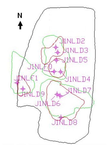
Acknowledgements

   This document was prepared by the Deep Vadose Zone-Applied Field Research Initiative at Pacific
Northwest National Laboratory. Funding for this work was provided by the U.S. Department of Energy,
Richland Operations Office. The Pacific Northwest National Laboratory is operated by Battelle
Memorial Institute for the U.S. Department of Energy under contract DE-AC05-76RL01830.

    The support of the U.S. Department of Energy, Richland Operations Office (Greg Sinton and Tom
Post) and the U.S. Environmental Protection Agency (Laura Buelow) is appreciated in facilitating project
efforts to meet aggressive schedules for implementation of the study. Valuable logistical support and
related excavation and groundwater data needed for conducting the project was provided by CH2M HILL
Plateau Remediation Company and Washington Closure Hanford personnel. Energy Solutions, Inc.
provided the direct-push drilling for the project.

                                                   v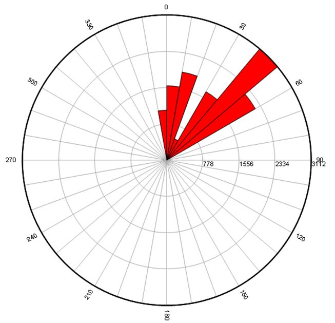
Contents

Executive Summary ..............................................................................................................................         iii
Acknowledgements ...............................................................................................................................          v
1.0 Introduction ..................................................................................................................................       1
2.0 Objectives .....................................................................................................................................      1
3.0 Background...................................................................................................................................         1
       3.1 Site Description and Conditions ...........................................................................................                    1
       3.2 Soil Contaminant Conditions ...............................................................................................                    2
4.0 Methods ........................................................................................................................................      3
       4.1 Aquifer Tube Cr(VI) Data ....................................................................................................                  4
       4.2 Drilling and Well Installation ...............................................................................................                 7
               4.2.1 Aquifer Tube and Well Locations .............................................................................                        7
               4.2.2 Drilling ......................................................................................................................      8
               4.2.3 Well Installation ........................................................................................................          11
               4.2.4 Well Development.....................................................................................................               12
               4.2.5 Well Modifications and Final Decommissioning ......................................................                                 12
       4.3 Hydraulic Testing and Groundwater Flow Direction/Gradient ............................................                                        13
               4.3.1 Constant-Rate Injection Tests ...................................................................................                   13
               4.3.2 Groundwater Flow Direction and Gradient ...............................................................                             14
               4.3.3 Electromagnetic Borehole Flow Meter .....................................................................                           15
       4.4 Tracer Tests ..........................................................................................................................       17
       4.5 Modeling Configuration .......................................................................................................                19
5.0 Results ..........................................................................................................................................   22
       5.1 Cr(VI) Concentration, Mass, and Flux .................................................................................                        23
               5.1.1 Vertical Profiling .......................................................................................................          23
               5.1.2 Temporal Cr(VI) Data ...............................................................................................                24
       5.2 Geology ................................................................................................................................      28
       5.3 Groundwater Flow Direction and Gradient ..........................................................................                            29
       5.4 Local-Scale Hydrologic Characterization ............................................................................                          31
               5.4.1 Electromagnetic Borehole Flow Meter Results.........................................................                                31
               5.4.2 Hydraulic Testing ......................................................................................................            38
               5.4.3 Tracer Tests ...............................................................................................................        40
               5.4.4 Modeling Interpretation of the Tracer Test ...............................................................                          49
6.0 Conclusions and Recommendations .............................................................................................                        55
       6.1 Summary of Study Information............................................................................................                      55

                                                                              vii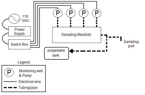
6.2 Cr(VI) Plume Interpretations ...............................................................................................                   57
               6.2.1 Downgradient Fluxes ................................................................................................                 57
               6.2.2 Correlation to Well 199-B4-14 Data .........................................................................                         58
       6.3 Recommendations ................................................................................................................               59
7.0 References ....................................................................................................................................       59

                                                                      Figures

1      Aerial photo of the existing 100-C-7 and 100-C-7:1 excavations looking to the south................                                                 2
2      Soil sample data at the floor of the 100-C-7:1 waste site .............................................................                             3
3      Locations of aquifer tubes for sample collection ..........................................................................                         5
4      Photo of the direct push technology drill rig that was used during drilling and installation
       of the 100-C-7:1 temporary small-diameter well network............................................................                                  9
5      Plan view of the 100-C-7:1 well network and nearby aquifer tubes .............................................                                     9
6      Nominal cross section of the 100-C-7:1 test site showing the relative well locations and
       screen depths .................................................................................................................................    10
7      Each well was developed by alternating the use of a dual flange surge block and
       Grundfos Redi-Flo2 submersible pump ........................................................................................                       12
8      Location of water-level monitoring wells relative to the 100-C-7 and 100-C-7:1 sites ...............                                               15
9      Schematic drawing of the groundwater sample acquisition system..............................................                                       19
10     Plan view of the numerical model grid showing boundary condition cells, the injection
       well, and locations of wells and nearby aquifer tubes ..................................................................                           20
11     Vertical profiling data from May 10, 2012 ...................................................................................                      23
12     Comparison of May 8 and May 10, 2012, vertical profiling data for Cr(VI) ...............................                                           24
13     Cr(VI) concentrations measured at aquifer tubes during sampling from May through
       August 2012 ..................................................................................................................................     26
14     Correlation of total chromium concentration results between laboratory and Hach
       Cr(VI) assays and between filtered and unfiltered laboratory assays ...........................................                                    27
15     East-west transect showing the water table and the Hanford/Ringold Formation contact............                                                   28
16     Hydraulic head data for wells 199-B4-14, 199-B5-8, and 199-B8-6 along with the
       corresponding groundwater flow direction calculated from the head data using
       “three-point problem” techniques .................................................................................................                 29
17     Groundwater flow direction and hydraulic gradient calculated from the hydraulic head
       data for wells 199-B8-6, 199-B4-14, and 199-B5-8 using “three-point problem”
       techniques .....................................................................................................................................   29
18     Radial frequency histogram depicting the groundwater flow direction in 10° bins as
       calculated from the hourly hydraulic head data for wells 199-B8-6, 199-B4-14, and
       199-B5-8 .......................................................................................................................................   30
19     Calculated hydraulic gradient and groundwater flow direction from hydraulic head data
       at wells 199-B8-6, 199-B4-14, and 199-B5-8 during the study period ........................................                                        30

                                                                             viii
20 Estimated groundwater velocities in the Hanford formation beneath the 100-C-7 and
100-C-7:1 excavations based on calculated hydraulic gradients and hydraulic property
estimates........................................................................................................................................ 31
21 Ambient vertical wellbore flow profiles for well UG1 before and after well reconfiguration ..... 33
22 Ambient vertical wellbore flow profiles for well CG1 before and after well reconfiguration ..... 33
23 Ambient vertical wellbore flow profiles for well DG1 before and after well reconfiguration ..... 34
24 Ambient vertical wellbore flow profiles for well DG2 before and after well reconfiguration ..... 34
25 Ambient vertical wellbore flow profiles for well INJ before and after well reconfiguration ....... 35
26 Normalized hydraulic conductivity profile for well UG1 prior to well reconfiguration .............. 36
27 Normalized hydraulic conductivity profile for well CG1 prior to well reconfiguration ............... 36
28 Normalized hydraulic conductivity profile for well DG1 prior to well reconfiguration .............. 37
29 Normalized hydraulic conductivity profile for well DG2 prior to well reconfiguration .............. 37
30 Normalized hydraulic conductivity profile for well INJ prior to well reconfiguration ................ 38
31 Observed pressure response in observation well CG1 for test in stress well INJ, with
fitted Neuman type-curve ............................................................................................................. 39
32 Observed pressure response in observation well DG1 for test in stress well INJ, with
fitted Neuman type-curve ............................................................................................................. 39
33 Observed pressure response in observation well INJ for test in stress well CG1, with
fitted Neuman type-curve ............................................................................................................. 40
34 Tracer injection rate and measured bromide concentration during tracer test 1 ........................... 41
35 Tracer test 1 monitoring results during the injection phase for both discrete groundwater
samples and the downhole probes................................................................................................. 42
36 Comparison of data for groundwater samples and the downhole probes for wells DG2
and INJ .......................................................................................................................................... 42
37 Arrival curves for INJ and DG2 based on downhole probe data that has been filtered to
remove artifacts resulting from groundwater sampling ................................................................ 43
38 Plot depicting an example of how the 50% arrival times were calculated; data in the vicinity
of the 50% relative concentration were fit to a linear equation, which was then used to
back-calculate the time for a relative concentration of 50% ......................................................... 43
39 Downhole probe data for well DG1 during tracer test 1 ............................................................... 44
40 Arrival and elution curves measured during tracer test 2 ............................................................. 47
41 Tracer concentration in well CG2 during tracer test 3 .................................................................. 48
42 Data for tracer test 2 showing the arrival data at wells DG2, INJ, and CG1 and elution
data for the injection well DG1 along with the corresponding smoothed data fits ....................... 50
43 Arrival curves for wells DG2, INJ, and CG1 in tracer test 2 for simulations with varying
porosity values .............................................................................................................................. 51
44 Arrival curves for wells DG2, INJ, and CG1 in tracer test 2 for simulations with varying
longitudinal hydraulic conductivity values ................................................................................... 52
45. Arrival curves for wells DG2, INJ, and CG1 in tracer test 2 for simulations with varying
dispersivity values......................................................................................................................... 52
46 Elution curves for well DG1 in tracer test 2 for simulations with varying porosity values .......... 53
ix47 Elution curves for well DG1 in tracer test 2 for simulations with varying hydraulic
conductivity values ....................................................................................................................... 54
48 Elution curves for well DG1 in tracer test 2 for simulations with varying dispersivity
values ............................................................................................................................................ 54
49 Comparison of tracer test 3 data to the corresponding simulation results .................................... 55
Tables
1 Sample collection requirements for aqueous water quality samples ............................................ 6
2 Analytical requirements for aqueous water quality samples ........................................................ 7
3 Elevation information for wells installed at the 100-C-7:1 site .................................................... 11
4 Sample collection requirements for aqueous tracer test samples .................................................. 18
5 Analytical requirements for aqueous tracer test samples .............................................................. 18
6 Descriptive parameters for the numerical model grid ................................................................... 20
7 Information about the tracer tests and numerical model configuration ........................................ 21
8 Cr(VI) concentrations based on aquifer tube sampling and field analyses performed
from May through August 2012 ................................................................................................... 25
9 Average of AT-1 through AT-7 Cr(VI) concentrations at specific sampling depths ................... 27
10 Summary of pertinent EBF test information ................................................................................. 32
11 Summary of ambient EBF survey results ..................................................................................... 35
12 Summary of hydraulic conductivity estimates from constant-rate injection tests in
100-C-7:1 wells conducted in August 2012.................................................................................. 39
13 Simplified calculation of the drift velocity based on the elution time at well DG1 and the
effective porosity and hydraulic conductivity based on arrival times during tracer test 1............ 45
14 Simplified calculation of the drift velocity based on the elution time at well DG1 and the
effective porosity and hydraulic conductivity based on arrival times during tracer test 2............ 48
15 Simplified calculation of the drift velocity and hydraulic conductivity based on tracer
elution measured during tracer test 3 ............................................................................................ 49
16 Values of parameters tested in the simulation matrix ................................................................... 50
17 Hydrologic data used in the Cr(VI) flux calculation..................................................................... 57
18 Cr(VI) concentrations at specific depth intervals for aquifer tubes AT-4, AT-5, AT-6,
and AT-7 based on samples collected in May, June, and July/August 2012 ................................ 58
19 Cr(VI) mass information determined from flux plane calculations for aquifer tubes AT-4,
AT-5, AT-6, and AT-7 based on data in Table 17 and Table 18 .................................................. 58
x1.0 Introduction
Deep excavation of soil has been conducted at the 100-C-7 and 100-C-7:1 waste sites within the
100-BC Operable Unit at the U.S. Department of Energy (DOE) Hanford Site to remove hexavalent
chromium (Cr(VI)) contamination with excavations reaching to near the water table. Soil sampling
showed that Cr(VI) contamination was still present at the bottom of the 100-C-7:1 excavation site. In
addition, Cr(VI) concentrations in a downgradient monitoring well have shown a transient spike of
increased Cr(VI) concentration following initiation of excavation. Potentially, the increased Cr(VI)
concentrations in the downgradient monitoring well are due to Cr(VI) from the excavation site. However,
data are needed to evaluate this possibility and to quantify the overall impact of the 100-C-7:1 excavation
site on groundwater. Several types of data were collected to assess the release of Cr(VI) from the
excavation site into the groundwater and impact on the groundwater quality. These data included
1) spatial and temporal Cr(VI) concentration data from the shallow groundwater beneath the
100-C-7:1 excavation; 2) hydraulic and tracer response data for characterization of local-scale
groundwater flow and contaminant transport; and 3) hydraulic gradient data.
The study described herein was conducted opportunistically while the 100-C-7:1 excavation was
accessible for characterization activities. Because the excavation was advanced to near the water table,
methods applicable for shallow subsurface investigation became feasible for use in studying the Cr(VI)
concentrations and hydraulic properties of the aquifer within the Hanford formation. The study was
initiated in April 2012 and completed in September 2012.
2.0 Objectives
The study was conducted with the following objectives:
• Quantify the release of Cr(VI) from the excavation site to the groundwater in terms of contaminant
mass discharge into the downgradient aquifer.
• Provide hydraulic property and groundwater flow and gradient estimates for the Hanford formation
aquifer beneath the 100-C-7:1 excavation site.
3.0 Background
3.1 Site Description and Conditions
The 100-C-7 and 100-C-7:1 waste sites were excavated to remove soil contaminated with Cr(VI).
These excavations removed soil down to the water table, a total excavation depth of about 26 m (85 ft)
below the original ground surface (Figure 1). No additional excavation is planned for 100-C-7 because
verification sampling shows that soil cleanup levels for Cr(VI) have been achieved. Continued
excavation in the upper portion of 100-C-7:1 is planned for the future. In addition, soil Cr(VI)
contamination above soil cleanup levels was identified at the bottom of 100-C-7:1; however, deeper
excavation could not continue because the bottom of the waste site had reached the water table.
1Figure 1. Aerial photo of the existing 100-C-7 and 100-C-7:1 excavations (April 2012) looking to the
south
Standard excavation processes were applied at these sites, including the addition of water for dust
control purposes.
The 100-C-7:1 excavation floor elevation of nominally 122 m above mean sea level (msl) was above
the water table in April 2012. However, the water table elevation increased and began flooding the
excavation in May. The excavation floor remained underwater from mid-May 2012 through the end of
the study period.
3.2 Soil Contaminant Conditions
Soil contamination data were collected in March 2012 at the floor of the 100-C-7:1 waste site with
sample locations J1NLD4, J1NLD5, J1NLD7, J1NLD9, J1NLF0, and J1NLF1 showing concentrations
above 10 mg/kg up to a maximum at J1NLD7 of about 40 mg/kg (Figure 2). These samples were
collected from approximately 7.5 cm below the excavation floor in the rewetted zone. Verification
sampling for the 100-C-7 site shows that soil cleanup levels for Cr(VI) have been achieved.
2Figure 2. Soil sample data at the floor of the 100-C-7:1 waste site. The black line is the floor outline.
The red lines show interpreted contamination zones from the March 2012 excavation floor
sample results. The green lines show interpreted contamination zones from previous higher-
elevation sample results. Sample locations are shown for the March 2012 sampling of the
excavation floor. Soil data and interpretations were provided by Washington Closure
Hanford.
4.0 Methods
There were three elements to the investigation.
Element 1. Spatially and temporally distributed Cr(VI) data in the shallow groundwater (top 1–3 m
of aquifer) were collected using aquifer tubes. In addition to spatial and temporal Cr(VI) data in the
shallow aquifer, aquifer tubes were also used to collect a vertical profile of Cr(VI) concentrations to a
depth of approximately 3 m.
Element 2. Local-scale hydrologic data were collected by installing a temporary network of small-
diameter monitoring wells (by direct-push drilling methods) at the bottom of the entrance ramp (above
high water level). The well network was installed to characterize the upper portion of the Hanford
formation, which is present at the water table. Measurements collected during direct-push drilling,
hydraulic testing, and tracer injection and natural gradient drift testing were analyzed to provide estimates
for the following:
• Elevation of the contact between the Hanford and Ringold Formations
• Effective porosity
• Groundwater velocity and associated hydraulic gradient
• Hydraulic properties (hydraulic conductivity, specific yield).
Element 3. A water-level monitoring network in the vicinity of the excavation (wells 199-B8-6,
199-B4-14, and 199-B5-8) was used to monitor hydraulic heads throughout the life of the project. These
3data were used to calculate the hydraulic gradient and groundwater flow direction that were used in
conjunction with the localized hydraulic property information, tracer data, and Cr(VI) concentration data
to assess release of Cr(VI) from the excavation site to the groundwater and estimate impacts to the
downgradient aquifer.
Following a series of planning and coordination meetings and subsequent DOE approval to start
work, project activities initially focused on installing a network of aquifer tubes so that baseline Cr(VI)
concentrations could be measured before the excavation was flooded with groundwater. Although a
longer baseline period would have been preferable, aquifer tubes were installed in time to monitor
elevated Cr(VI) concentrations that were mobilized as the water table came into contact with excavation
bottom sediments. This aquifer tube network was routinely monitored over the duration of the project.
A temporary, small-diameter monitoring well network was installed (by direct-push drilling methods)
for determination of local-scale hydraulic and transport property estimation. The well network, which
was located directly adjacent to the excavation on an elevated access road, was originally designed to
focus interrogation on a 3-m (10-ft) interval of Hanford formation, the top of which was the approximate
elevation of the excavation floor. Results from initial hydraulic and tracer testing in this well network
revealed that the Hanford formation was most transmissive near the water table, and that another zone of
increased permeability near the bottom of the 3-m (10 ft) screened interval resulted in significant vertical
wellbore flow in these wells under ambient conditions. Because the observed wellbore flows
significantly impacted the concentration of tracers measured in the monitoring wells and limited the
ability to quantitatively assess natural gradient tracer drift response data, the wells were reconfigured
using bentonite fill material to decrease the test interval to the upper 1.5 m of each 3-m well screen. This
reconfigured well network, which effectively mitigated the ambient wellbore flow problem and focused
hydrologic interrogation on the upper 1.5-m test interval, was then used to perform both hydraulic and
tracer injection and natural gradient drift tests. Results from these tests, along with hydraulic gradient
information from a well network in the vicinity of the site, were used to characterize properties
controlling local-scale groundwater flow and contaminant transport.
Field testing and monitoring activities conducted in support of the three project elements listed above
are discussed in more detail in the following sections.
4.1 Aquifer Tube Cr(VI) Data
Groundwater samples were collected and analyzed to determine Cr(VI) concentration. Eight lateral
sampling locations within the 100-C-7:1 excavation floor were selected for the installation of aquifer
tubes used to collect groundwater samples (Figure 3).
Vertical profiling of Cr(VI) concentration was conducted with a preliminary profiling on May 8,
2012, at location AT-1 and additional profiling on May 10, 2012, at locations AT-1, AT-3, and AT-6 to a
total depth of ~3.1 m (10 ft). Vertical profiling was conducted with a 1-in.-diameter drive rod and with
sampling every ~0.5 m (1.5 ft). Surface water samples were also collected at these locations. The drive
rod was advanced into a pre-dug 15-cm-deep hole. After the aquifer tube was below the bottom of the
hole, the hole was filled with coated bentonite pellets to create a surface seal during additional advance-
ment of the rod and sampling. Samples were analyzed for Cr(VI) using a field spectrophotometric
method (described in the following paragraphs).
4Figure 3. Locations of aquifer tubes for sample collection. Open circles indicate areas of elevated
Cr(VI) concentration from soil samples. Filled circles are downgradient monitoring locations.
Each of the primary eight monitoring locations consisted of at least two sample depth intervals with a
shallow well-point aquifer tube installed to a depth of about 1 m below the excavation floor and another
aquifer tube installed to a depth of 3 m. At locations AT-1, AT-6, AT-7, and AT-8, an additional aquifer
tube was installed to a depth of 2 m. Well-point aquifer tubes were used for the shallow sample depth
interval because the installation method did not require back-pulling of a drive rod and provided for a
better surface seal at these shallow depths. All abovementioned depths represent the depth from ground
surface to the middle of the screen. The well-point aquifer tubes were constructed of 3.2-cm ID stainless-
steel pipe with a 30-cm-long wire wrapped screen. A cap with a bulkhead fitting was attached to the top
of the well point to allow pass through of the sample tubing to the screened interval. Aquifer tubes were
constructed of 1-cm outside diameter polyethylene tube with a 30-cm screen interval. The screen was
constructed of 50-µm polyethylene mesh wrapped around perforations in the tubing. Aquifer tubes and
well-point aquifer tubes were installed using methods previously developed for sampling along the
Columbia River shoreline (Fritz et al. 2007). Surface completion at all aquifer tube locations consisted of
emplacing a bentonite surface seal, as described for the vertical profiling above, to prevent surface water
from moving vertically along the aquifer tube during sampling. In addition to the eight primary sampling
locations, seven aquifer tubes were installed near the well field to provide supplemental monitoring for
the natural gradient tracer testing. Four of these aquifer tubes (AT-9, -10, -11, -12) were installed with
the screen midpoint at an elevation of 121.5 m, which is the approximate midpoint of the original well
5network’s 3-m (10-ft) screen intervals. Three additional tubes (AT-13, -14, and -15) were installed with
the screen at the approximate midpoint of the reconfigured well network test interval (i.e., upper 1.5 m
[5 ft] of the original screen interval). The location of these aquifer tubes (on the slope near the access
road) required a deeper installation depth than the other shallow installations, but the elevation of the
aquifer tubes was comparable to that of the shallow well points at the other eight sampling locations. The
installation and completion of these seven aquifer tubes was comparable to that of the eight primary
locations.
Groundwater samples were pumped from the aquifer tubes using a peristaltic pump. Purge times
were scaled according to the tubing length and flow rate such that two to three tubing volumes were
purged prior to sample collection. During sample collection, field parameters (specific conductance, pH,
dissolved oxygen, and oxidation reduction potential) were measured using a flow-through cell (model
MP20, QED Environmental Systems, Ann Arbor, Michigan) and monitored for stability. The dissolved
oxygen and oxidation reduction potential values were consistently above 7 mg/L and 150 mV,
respectively, indicating suitable (oxic) conditions for collection of Cr(VI) samples. The probe was
calibrated for specific conductance and pH prior to each sampling event. Field parameters were hand-
recorded on a field data sheet and transferred to an electronic data file at the completion of field activities.
After recording the field parameters, a sample was collected in a clean, triple-rinsed glass beaker. The
sample was then divided into three sub-samples; a filtered/acidified sample, an unfiltered acidified
sample, and a filtered sample for field analysis of Cr(VI).
Aqueous sample collection and analytical requirements are shown in Table 1 and Table 2,
respectively. Measurement of Cr(VI) occurred in the field less than 1 hour after sample collection.
Concentrations of Cr(VI) were measured using spectrophotometric methods (model DR 2000, Hach Co.,
Loveland, Colorado). The filtered sample was transferred to a reagent bottle and allowed to sit for 5 min.
During this time, Cr(VI) present in the sample reacted with the reagent, turning the sample purple.
Table 1. Sample collection requirements for aqueous water quality samples
Parameter Media/Matrix Sampling Frequency(a) Volume/Container Preservation
RCRA/Trace Metals: Water Collected for all samples; 25-mL plastic vial Filtered and
Cr subset selected for analysis (acid washed) unfiltered,
HNO3 to pH < 2
Hold time: 60 days
Cr(VI) Water 10 sampling events, varying Field measurement Filtered
frequency
pH Water Measure for all samples Field measurement None
collected
Electrical conductivity Water Measure for all samples Field measurement None
collected
Dissolved oxygen Water Measure for all samples Field measurement None
collected
Oxidation reduction Water Measure for all samples Field measurement None
potential collected
(a) Sampling frequency for temporal monitoring, not profiling.
QC = quality control; RCRA = Resource Conservation and Recovery Act.
6Table 2. Analytical requirements for aqueous water quality samples
Typical
Parameter Analysis Method Detection Limit Precision/Accuracy QC Requirements
RCRA/Trace Metals: ICP-MS, 1 µg/L for trace ±10% Daily calibration;
Cr PNNL-AGG-415 elements blanks and duplicates
(similar to EPA and matrix spikes at
Method 6020) (EPA 10% level
2007)
Cr(VI) Hach DR-2000 w/ 10 µg/L ±10 µg/L Blanks, duplicates at
Accuvac Ampules 10% level
pH pH electrode Not applicable ±0.1 pH unit User calibrate
Electrical conductivity Electrode 1 µS/cm ±10% User calibrate
Dissolved oxygen Membrane electrode 0.1 ppm ±15% For indication only
Oxidation reduction Electrode Not applicable ±10% For indication only
potential
QC = quality control; RCRA = Resource Conservation and Recovery Act.
The intensity of the purple color was proportional to the Cr(VI) concentration, which was quantified
by the spectrophotometer instrument. The measured concentrations were also hand-recorded on the field
data sheet and transferred to an electronic data file at the completion of field activities. Archived samples
were held for laboratory analysis of total chromium (Table 1). A sub-set of the archived samples were
selected for total chromium analysis by inductively coupled plasma mass spectrometry (ICP-MS)
(Table 2).
4.2 Drilling and Well Installation
This section summarizes activities related to the drilling, construction, and decommissioning of the
100-C-7:1 well network.
4.2.1 Aquifer Tube and Well Locations
Horizontal and vertical coordinates of the aquifer tubes and wells were either mapped for
approximate location or surveyed for a more precise coordinate. The horizontal coordinates of the eight
primary aquifer tube monitoring locations on the excavation floor (AT-1 through -8) were mapped using a
hand-held global positioning system (GPS; model Montana 650t, Garmin Ltd., Olathe, Kansas). The GPS
receiver reported a horizontal accuracy of about ±5 m when these locations were mapped. The elevation
of the ground surface for these eight points was based on elevation contours from the civil survey
obtained from Washington Closure Hanford (Figure 3).1
The seven aquifer tubes located near the well field (AT-9 through -15) and the six wells were
surveyed using an electronic total station (model Set330R, Sokkia Corp., Olathe, Kansas) with an overall
horizontal and vertical accuracy of about ±0.02 m. The horizontal coordinates for these points are relative
1
Martinez C. 2012. E-mail to Rob Mackley (Pacific Northwest National Laboratory) from Charlene Martinez
(Washington Closure Hanford), “Locations of aquifer tubes for sample collection,” May 7, 2012, Richland,
Washington.
7x-y positions – no control was used to reference the horizontal coordinates into the “real world” (e.g.,
latitude/longitude). These relative horizontal coordinates were used to calculate radial distances and
bearings between the injection and monitoring wells and aquifer tubes. The vertical coordinates of these
locations were converted to real-world elevations based on water table elevation according to the
following steps:
1. The known top of casing elevation for well 199-B8-6 from the Hanford Well Information System was
combined with a depth-to-water measurement (using the same e-tape as described in Section 4.3.2) to
calculate the water table elevation.
2. The depth-to-water was measured in well DG2 within 5 min of the measurement in well 199-B8-6.
The water table in the two wells was assumed to be similar in elevation (within the error of the
survey) due to their close proximity (about 300 m).
3. The depth-to-water in well DG2 was added to the water table elevation to find the unknown elevation
of the top of the well casing.
4. All vertical survey measurements with the total station were referenced to the top of casing elevation
for well DG2 and converted to a real-world elevation (NAVD88).
4.2.2 Drilling
A network of six temporary, small-diameter wells was installed near the bottom of the entrance ramp
to the 100-C-7:1 excavation site to support aquifer hydraulic/tracer testing. All of the borings were
drilled and wells installed during a single drilling campaign using direct-push technology (DPT) drilling
methods (Figure 4). Each boring was advanced to total depth using nominally sized 7.6-cm-(3-in.-)
diameter carbon steel temporary casing fitted with a 10.8-cm (4 1/4-in.) diameter drive point that was
knocked out and left in place prior to well installation. The well network (Figure 5 and Figure 6) consists
of one central well (INJ) through which initial tracer injection testing was conducted, three shallow near-
field monitoring wells (DG1, UG1, and CG1), one shallow far-field monitoring well (DG2), and one deep
near-field monitoring well (CG2). All shallow wells were completed with 3-m (10-ft) screens, nominally
placed between elevations of 119 m to 122 m above msl. The top of this interval is the approximate
elevation of the excavation bottom. To monitor for vertical migration of injected tracer solution, one deep
near-field monitoring well was completed with a 0.6-m (2-ft) screen interval placed from 116.4 m to
117.0 m above msl.
8Figure 4. Photo of the direct push technology drill rig that was used during drilling and installation of
the 100-C-7:1 temporary small-diameter well network
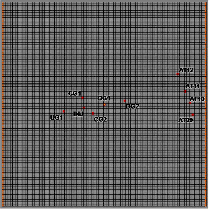
Figure 5. Plan view of the 100-C-7:1 well network and nearby aquifer tubes. Numbers in parentheses
indicate the radial distance from the INJ well in meters. The notation “H/R” refers to the
contact between the Hanford and Ringold Formation geologic units. The line of wells UG1,
INJ, DG1, and DG2 lie along an azimuth of 35°.
9Vertical profile sampling of Cr(VI) was conducted at discrete depth intervals while advancing the
temporary drill casing for the installation well DG2. A total of four groundwater samples were collected
at 2.6, 3.5, 12.0, and 15.4 m (8.5, 11.5, 39.5, and 50.5 ft, respectively) below the top of the water table,
which itself was 3.8 m (12.5 ft) below ground surface. To characterize Cr(VI) concentrations closer to
the groundwater surface, an additional sample was collected from well DG1 at approximately 0.6 m (2 ft)
below the water table. None of the samples collected during drilling contained measurable Cr(VI)
concentrations. All groundwater samples were collected and Cr(VI) concentrations were measured in the
field using the methods described in Section 4.1.
Figure 6. Nominal cross section of the 100-C-7:1 test site showing the relative well locations (with CG1
and CG2 projected onto the cross section) and screen depths. The figure is not to scale.
Elevations are in meters; screen lengths are 3 m (10 ft) and 0.6 m (2 ft). The notation “H/R”
refers to the contact between the Hanford and Ringold geologic formations (fm). Bentonite
material was used to reconfigure the 3-m (10-ft) well screens to 1.5-m (5-ft) screens.
104.2.3 Well Installation
Each well was constructed using 5-cm-(2-in.-) diameter polyvinyl chloride (PVC) casing
(Schedule 40, ASTM D1785, F480 with flush-threaded joints and Viton “O” rings) and 20-slot (0.05-cm
[0.020-in.]) PVC screens (ASTM D1785, F480, continuous wire wrap, with flush-threaded joints and
Viton “O” rings); no glues or solvents were used. Filter pack material consisted of 10-20 mesh filter pack
sand. These selections were based on the hydrogeology encountered during drilling, as well as
information from nearby wells.
Filter pack installation and initial well development consisted of introducing silica sand into the
annular space around the screen and settling the filter pack to eliminate void spaces. A dual-flange surge
block was used to develop and settle the filter pack in the annular space between the screen and the
borehole wall. Surging of the 3-m (10-ft) screens was carried out in two stages, developing the screen in
1.5-m (5-ft) intervals. The 0.6-m (2-ft) screen installed at well CG2 was developed in one stage.
The five shallow wells (INJ, UG1, CG1, DG1, and DG2) were constructed with a hydrated bentonite
crumble seal placed above each screen’s filter pack interval to ground surface. However, the single deep
well (CG2) required an alternate construction method to install an annular seal because the top of the
filter pack material was located too far below the water table to use bentonite crumbles without the risk of
bridging, and the annular space was too small to accommodate bentonite chips or pellets. For this reason,
bentonite slurry was mixed at the surface and pumped down the annular space using a peristaltic pump.
To prevent intrusion of bentonite slurry into the filter pack, approximately 0.15 m (0.5 ft) of 20-40 mesh
silica sand was placed above the 10-20 mesh filter pack prior to pumping bentonite slurry. Bentonite
slurry was pumped and allowed to settle to within 0.15 m (0.5 ft) of the ground surface, and then covered
with a hydrated bentonite crumble seal at the surface. Because all six wells were temporary completions,
surface casing and protective bollards were not installed. Each well was completed with 0.15 m to 0.46 m
(0.5 to 1.5 ft) of stickup above ground surface and fitted with a J-plug type well cap. Additional details
are provided in Table 3.
Table 3. Elevation information for wells installed at the 100-C-7:1 site
Approx. Elevation of the
Approx. Ground Groundwater Elevation of the Top of Bottom of the Well
Well Surface Elevation Elevation the Well Screen Screen
Name (m msl) (m msl) (m msl) (m msl)
UG1 126.99 122.57 121.92 118.97
INJ 126.72 122.59 121.98 118.93
CG1 126.76 122.44 121.91 118.87
CG2 126.67 122.63 117.02 116.41
DG1 126.49 122.60 122.16 119.11
DG2 126.19 122.60 122.01 118.96
m msl = meters mean sea level.
114.2.4 Well Development
Final well development was performed by alternating the use of a dual flange surge block and a
Grundfos Redi-Flo2 submersible pump (Figure 7) to develop the wells until groundwater clarity was
determined sufficient and field parameters, including temperature and conductivity, had stabilized. Water
level drawdown during development was monitored periodically using an electronic tape measure.
During development, the pump was operated with the intake located at multiple stages within the
screened intervals. The flow rates were measured at approximately 11.4–13.2 L/min (3.0–3.5 gallons per
min [gpm]) with less than 3 cm (0.10 ft) of drawdown.
Figure 7. Each well was developed by alternating the use of a dual flange surge block (on the ground by
the well in this photo) and Grundfos Redi-Flo2 submersible pump (down-hole in this photo)
4.2.5 Well Modifications and Final Decommissioning
After the results of the initial tracer test were evaluated, Electromagnetic Borehole Flow meter (EBF)
testing was conducted to evaluate the vertical distribution of horizontal hydraulic conductivity within
each well. Based on the results of the EBF testing (see Section 5.4.1), a decision was made to modify the
well network by plugging the bottom half of the 3-m (10-ft) screen intervals. A 1.5-m (5-ft) seal was
installed in each well using coated bentonite pellets, and then covered with 0.15 m (0.5 ft) of washed pea
gravel to protect downhole equipment from coming into contact with the bentonite. After completion of
the final injection tracer test, all wells were decommissioned by backfilling the 5-cm (2-in.) screen and
PVC casing with 1-cm (3/8-in.) bentonite chips, and either unthreading and removing the surface joint of
5-cm (2-in.) PVC casing, or cutting the 5-cm (2-in.) PVC casing flush to the ground. No permanent
markings were installed because the excavation pit will be backfilled to original ground surface beginning
in the fall of 2012.
124.3 Hydraulic Testing and Groundwater Flow Direction/Gradient
Hydrologic characterization activities performed in support of this study are discussed in detail in the
following sections.
4.3.1 Constant-Rate Injection Tests
A series of constant-rate injection tests were performed in multiple wells in June and August 2012 to
estimate local-scale aquifer hydraulic properties beneath the field test site. June testing consisted of a
constant-rate injection test in well INJ prior to reconfiguration of the wells (i.e., the test was for a 3-m
[10-ft] screened interval). Results from the June tracer injection test and EBF profiles indicated a
relatively high permeability interval over the upper portion of the aquifer and significant ambient vertical
wellbore flows in the wells (Section 5.4.1). The wells were reconfigured in July by plugging the bottom
half of the screens with bentonite to reduce the effective screen interval to the upper 1.5 m of the original
screened interval where the highest permeability materials were indicated. In August 2012, constant-rate
injection tests were performed in the reconfigured well network; quantitative analysis of hydraulic test
responses focused on these test results because 1) this test interval is consistent with that interrogated
during the quantitative tracer testing; and 2) this shallow interval is considered of primary interest for
Cr(VI) transport.
The constant-rate injection tests were designed to maximize the observable pressure response and
minimize the surface boundary effects of the ponded water in the nearby excavation, the boundary of
which was about 15 m away. The floor of the excavation was below the water table during the higher-
water conditions from May to November (see hydrographs in Section 5.3). During the hydraulic tests in
August, there was more than a meter of ponded water covering the excavation floor. Screening
calculations indicated that there would be a noticeable effect on the pressure responses within only a few
minutes of test initiation and that this boundary effect would need to be accounted for in the analysis. For
this reason, the tests were limited to a 40-min injection period, followed by about the same amount of
time for pressure recovery.
Ponded water from the excavation was extracted and pumped through filters and into the stressed
wells using two 4-in.-diameter submersible pumps in parallel. Injection pressures and flow rates were
monitored within the same process trailer equipment used in the tracer injection testing (see Section 4.4).
Flow rates of 37 and 42 gpm were held constant during the tests in stress wells INJ and CG1,
respectively. Pressure buildup and recovery were monitored in the stress well and nearby observation
wells using submersible pressure sensors (model CT2X, Instrumentation Northwest, Kirkland,
Washington).
Hydraulic properties were estimated using a type-curve fitting method according to the analytical
solution of Neuman (1972, 1974, 1975) for an unconfined aquifer with delayed gravity response (specific
yield). In this analysis, the wells can be either partially or fully penetrating. The analysis assumes the
aquifer is homogeneous, of infinite areal extent, of uniform thickness, and ignores well-bore storage
effects. The Neuman type-curve analyses were conducted using the aquifer test analysis software
AQTESOLV (HydroSOLVE, Inc., Reston, Virginia). Type curves were fit to the pressure recovery data
rather than data from the pressure buildup (injection) phase because these data typically have less
13variability, particularly in the early portion of the test response. Prior to analysis, the recovery data were
translated to an equivalent pumping test response through the Agarwal (1980) correction method.
The effective aquifer thickness used in the analysis was determined based on the combination of
results from EBF vertical profiling and tracer injection tests. EBF results indicated that the upper 1.5 m
of the original 3-m screened interval was most transmissive, with a zone from about 4.88 to 5.49 m (16 to
18 ft) below ground surface showing more than an order of magnitude higher relative hydraulic
conductivity than deeper in the formation (see Section 5.4.1). Results from an initial scoping-level tracer
injection (see Section 4.4) were generally consistent with the EBF results, showing relatively dispersed
tracer arrival fronts, which is consistent with the presence of flow system heterogeneities, and no
indication of tracer migration below the 3-m test interval (i.e., no tracer arrival was observed in well CG2,
which is screened approximately 1.5 m below the bottom of the test interval). Given this information, the
effective test interval for these tests was interpreted to be limited to the saturated material within and
above the reconfigured screen interval. The EBF profiles do not extend above the well screen elevation,
so the relative permeability of material above the screen is unknown. However, it was assumed that the
higher permeability materials indicated for the upper 1.5-m test interval extended to the water table. A
partial-penetration model with stress and observation wells having screened-intervals of 1.52 m (5 ft)
located at the base of a 2.74-m-(9-ft-) thick aquifer was used in the analysis. This conceptual model
appears reasonable based on the model fit to the observed data and the agreement of the hydraulic
conductivity estimates from this analysis with values obtained independently from the tracer drift analysis
(see Section 5.4.3). Conversely, a fully penetrating well configuration that assumes an aquifer thickness
of only 1.52 m (5 ft) would yield K estimates about two times those reported in the following paragraphs,
and would not be consistent with tracer test results.
Type curves were fit to the pressure responses in the observation wells using the Neuman solution
while adjusting specific yield (Sy) and transmissivity (T) values to improve the goodness of fit.
Storativity (S) and anisotropy (Kz/Kh) were prescribed to values of 0.001 and 0.1, respectively.
Hydraulic conductivity (K) values were calculated from the transmissivity (T) estimates using a
prescribed saturated thickness (b) of 2.74 m (9 ft) according to T = K/b.
As noted above, the wells are located within 15 m (50 ft) of the excavated pit that intersected the
aquifer at the time of testing. Surface water was ponded in the pit and created a constant-head boundary
condition. The analysis used superposition theory and image-well methods (Ferris et al. 1962) to account
for the effects of this boundary.
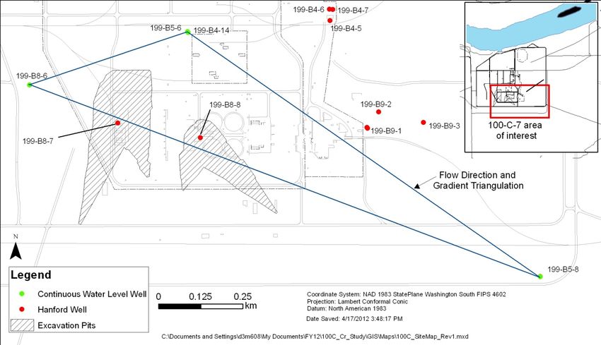
4.3.2 Groundwater Flow Direction and Gradient
Water-level data from nearby wells were used to determine the groundwater flow direction and
gradient in the 100-C-7:1 vicinity. The gradients and flow directions were calculated according to the
triangulation method described by Devlin (2003). There are a number of existing wells located nearby;
however, only three of these wells (199-B4-14, 199-B5-8, and 199-B8-6) were instrumented with
pressure transducers as part of CH2M HILL Plateau Remediation Company’s Hanford water-level
monitoring network (Figure 8). Continuous water-level data for these three wells were extracted from the
Automated Water Level Network module within the Virtual Library (http://vlprod.rl.gov). Data are
available in the Virtual Library starting in late 2010 and early 2011 for these three wells. Manual water-
level verifications in these wells taken with a National Institute of Standards and Technology-traceable
14electronic water level indicator (“e-tape”; RST Instruments, Maple Ridge, British Columbia, Canada)
agreed with the continuous data to within ±0.02 m. These differences are reasonable given the combined
errors associated with depth-to-water measurements, sensor miscalibration (drift/offset), and vertical
survey. Well coordinates were extracted from the Well Information and Document Lookup webpage
(http://prc.rl.gov/widl/).
Figure 8. Location of water-level monitoring wells relative to the 100-C-7 and 100-C-7:1 sites
4.3.3 Electromagnetic Borehole Flow Meter
EBF surveys are effective for measuring the vertical groundwater-flow velocity distribution in wells.
The vertical groundwater-flow velocity measurements can be used to infer the distribution of lateral
groundwater flow into the well. The objective of EBF surveys is to characterize the ambient (i.e., static)
or dynamic (i.e., pump-induced), in-well vertical flow conditions (i.e., vertical flow-velocity magnitude
and direction) within the saturated well-screen section. Dynamic EBF survey results corrected for
ambient flow conditions can be used to characterize the distribution of vertical flow conditions and
inferred vertical hydraulic conductivity distribution.
4.3.3.1 Electromagnetic Borehole Flow Meter Field Method
The theory that governs the operation of the EBF is Faraday’s Law of Induction, which states that the
voltage induced by a conductor moving at right angles through a magnetic field is directly proportional to
the velocity of the conductor moving through the field. In the EBF apparatus, flowing water is the
conductor, an electromagnet generates a magnetic field, and electrodes are used to measure the induced
voltage. For sign convention, upward flow represents a positive voltage signal and downward flow
represents a negative voltage signal. A more detailed description of the EBF instrument system and field
test applications are provided in Young et al. (1998).
15You can also read