Irradiance Volumes for Games - Natalya Tatarchuk 3D Application Research Group ATI Research, Inc - AMD Developer
←
→
Page content transcription
If your browser does not render page correctly, please read the page content below
Irradiance Volumes for Games
        Natalya Tatarchuk
     3D Application Research Group
            ATI Research, Inc.
Overview
• Introduction and Motivation
• Review
  – Radiance, Irradiance, Transfer
• Spherical Harmonics
  – Projection, Gradients, Evaluation
• Irradiance Volume
  – Uniform Subdivision, Adaptive Subdivision,
    Interpolation
• Summary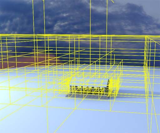
Motivation
• Real-time and offline rendering have one
  important gap: the use of global illumination for
  physically based, realistic lighting
• Games use light mapping
   – Approximates global illumination on the surface
   – Only for static scenes!
   – Does not address dynamic objects that move through
     the scene
   – Result in beautifully rendered, globally illuminated
     scenes that contain unrealistic, locally lit dynamic
     objects
• Solution:
   – Precomputed Irradiance Volumes for static scenes
   – Precomputed Radiance Transfer for objects within
     those scenes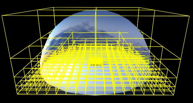
The Irradiance Volumes
• We aim to solve as much of the global
illumination calculation during preprocess
time
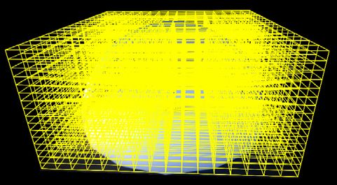
• A 3D light map: volume of diffuse lighting
samples
9 This is what we’re
trying to achieve
[Greger98]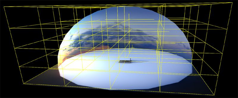
Used in Ruby: Dangerous
             Curves

•   These techniques were used as a drop in replacement
    for diffuse lighting in the Ruby: Dangerous Curves demo
•   At the very least, these techniques could serve as an
    ambient lighting solution in your games
•   Before diving into the details it is necessary to have a
    basic familiarity with the following terms:
     – Radiance, Irradiance, and Transfer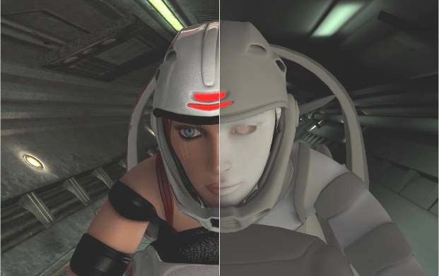
Demo

Ruby2: Dangerous Curves
Agenda
• Introduction and Motivation
• Review
   – Radiance, Irradiance, Transfer
• Spherical Harmonics
   – Projection, Gradients, Evaluation
• Irradiance Volume
   – Uniform Subdivision, Adaptive Subdivision,
     Interpolation
• Summary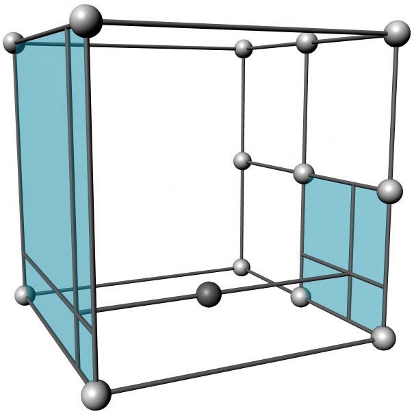
Radiance

                                             [Greger98]

• Radiance is the emitted energy per unit time in
  a given direction from a unit area of an emitting
  surface
Capturing Radiance
•   Capture radiance at a point for all
    directions
     – Place a camera at that point
     – Render the surrounding scene into a
       cubemap
     – Scale each texel by its projected solid
       angle
•   The cube map represents the radiance
    for all directions for this point
     – Known as the radiance distribution        [Greger98]
       function
     – Not necessarily continuous (Even in
       simple environments)
•   Every point in space has a radiance
    distribution function
     – Radiance is a 5D function (3 spacial
       dimensions and 2 directional
       dimensions)
Radiance

                                             [Greger98]

•   The radiance of a surface is a function of its BRDF and
    incident radiance
•   The incident radiance defined on the hemisphere of
    incoming directions is called the field-radiance function
Irradiance
• The radiance of a purely diffuse surface is defined in
terms of the surface’s irradiance
• Irradiance is an integral of the field-radiance function
multiplied by the Lambertian cosine term over a
hemisphere
r r
I ( p, N p ) = ∫ L( p, ωi )( N p • ωi )dωi
ΩIrradiance
[Greger98]
• We could compute irradiance at a point for all possible orientations of a
small patch:
– For each orientation, compute a convolution of the field radiance with a
cosine kernel
• The result of this convolution for all orientations would be an irradiance
distribution function
• The irradiance distribution function looks like a radiance distribution
function except much blurrier because of the averaging process
(convolution with cosine kernel)
• The irradiance distribution function is continuous over directionsIrradiance
• The irradiance distribution function can be computed for
every point in space: irradiance is a 5D function (3
spatial dimensions and 2 directional dimensions)
• Evaluating the irradiance distribution function in the
direction of a surface normal gives us irradiance at that
surface location
• Computing irradiance distribution functions on demand is
possible but can be costly. An obvious optimization is to
precompute irradiance distribution functions for a scene
at preprocess time and then use this precomputed data
at runtimeRendering with Irradiance
• The Irradiance Distribution Function at a point can be
stored using a “Diffuse Cube Map”
• The cube map is indexed with an object’s surface normalEfficient Storage of
Irradiance
• We need an irradiance distribution function for objects
moving in the scene
• Capture the lighting environment at many points in the
scene
– At preprocess time
– Then we’ll have a volume of irradiance distribution functions
• But! We’re still left with the cost of storing tons of cubemaps
– For all the points in the scene
– And the bandwidth overhead of indexing these maps at render
time
• Instead! Compress irradiance maps
– Represent each as a vector of spherical harmonic coefficients
– Reduces both storage and bandwidth costsAgenda
• Introduction and Motivation
• Review
– Radiance, Irradiance, Transfer
• Spherical Harmonics
– Projection, Gradients, Evaluation
• Irradiance Volume
– Uniform Subdivision, Adaptive Subdivision,
Interpolation
• SummarySpherical Harmonics
• Infinite series of spherical functions
• Can be used as basis functions
– Stores a frequency space approximation of an
environment map
• Use Microsoft DirectX SDK for spherical
harmonics computations
– Includes functions for projecting a cubemap into a
representative set of spherical harmonic coefficients
– Also functions for scaling and rotating spherical
harmonics – important if your object is moving
• For code snippets that will help your write your
own spherical harmonic helper functions, see
Robin Green’s Spherical Harmonic Lighting:
The Gritty DetailsFourier Theory
+
+
Sum of =
sine = Successive
waves Approximation
+
=
+
=
• Recall that it is possible to represent any 1D signal as a sum of
appropriately scaled and shifted sine waves
• Spherical harmonics are the same idea on a sphere!Spherical Harmonic Basis
Positive Values
Negative Values
From [Green]Spherical Projection:
Storage and Computation
[Ramamoorthi]
Original Filtered SH
Environment Environment Representation
Map Map
• Projecting an environment map into 3rd order spherical harmonics effectively
gives you the irradiance distribution function [Ramamoorthi]
• Projection into 3rd order SH is not only a storage win but a preprocessing win
too since SH projection is much faster than convolving an environment map
with a cosine kernel for all possible normal orientationsSpherical Harmonics
• Once an environment map has been projected into spherical
harmonics, the coefficients can be used to evaluate the original
map in a given direction
• Storing these coefficients VS constants allows us to compute
irradiance per-vertex rather than having to sample a cubemap
per-pixelSH Evaluation With
Normal
float4 cAr; // first 4 red irradiance coefficients
float4 cAg; // first 4 green irradiance coefficients
float4 cAb; // first 4 blue irradiance coefficients
float4 cBr; // second 4 red irradiance coefficients
float4 cBg; // second 4 green irradiance coefficients
float4 cBb; // second 4 blue irradiance coefficients
float4 cC; // last 1 irradiance coefficient for red, blue and green
float3 x1, x2, x3;
// Linear + constant polynomial terms
x1.r = dot(cAr, vNormal);
x1.g = dot(cAg, vNormal); Constant:
x1.b = dot(cAb, vNormal);
// 4 of the quadratic polynomials Linear:
float4 vB = vNormal.xyzz * vNormal.yzzx;
x2.r = dot(cBr, vB);
x2.g = dot(cBg, vB);
x2.b = dot(cBb, vB); Quadratic:
// Final quadratic polynomial
float vC = vNormal.x*vNormal.x - vNormal.y*vNormal.y;
x3 = cC.rgb * vC;
Output.Diffuse.rgb = x1 + x2 + x3;
[Shader Code From DirectX SDK]One Irradiance Sample: A
Point in Space
• Irradiance samples only store irradiance for a single
point in space
• This really only works well if the lighting environment is
infinitely distant (just like a cubic environment map)
• This error can be very noticeable when the lighting
environment isn’t truly distantSpherical Harmonic
Irradiance Gradients
• If an irradiance sample is used to shade the surface of an
object, the potential error increases the further we move away
from the point at which the irradiance sample was generated
• Irradiance gradients allow us to store the rate at which
irradiance changes with respect to translations about the
sampleIrradiance Gradients No Irradiance Gradients With Irradiance Gradients If irradiance varies greatly near a sample point, can store irradiance gradients along with each irradiance sample. [Ward 92][Annen04]
Spherical Harmonic
      Irradiance Gradients
•   Translational gradients for spherical harmonic irradiance
    samples may be computed in a number of ways [Annen]…
•   One simple way to find the gradients is to use central
    differencing to estimate the partial derivatives of the
    spherical harmonic irradiance coefficients
•   Project 6 additional irradiance functions into spherical
    harmonics and perform central differencing on each of the
    coefficients
Central Differencing
y+1 − y−1
d ∇y =
d
• Subtract the coefficients for samples taken at a small offset in
the +Y and –Y directions
• Divide by distance between the samples
• This gives you an estimate of the partial derivative with respect
to y for each coefficient
• Do this for the other two axes as well…
• You now have a 3D gradient vector for each spherical
harmonic coefficientFirst-Order Taylor
Expansion
• At render time, the gradient may be used to extrapolate a new
irradiance function
• Compute world space vector from the location at which the sample was
generated to the point being rendered
• This vector is then dotted with the gradient vector and added to the
original sample to extrapolate a new irradiance function
I i′ = I i + (∇I i ⋅ d )
• Ii’ is the ith spherical harmonic coefficient of the extrapolated irradiance
function, Ii is the ith spherical harmonic coefficient of the stored
irradiance sample, is the irradiance gradient for the ith irradiance
coefficient and d is a non-unit vector from the original sample location
to the point being rendered
∇I i// Compute vector from original irdiance sample position to the position that is being
shaded
float3 vSampleOffset = (vPos - vIrradianceSamplePosWS);
// Arrays for the extrapolated 4th order (16 coefficients per color channel) spherical
harmonic irradiance
float4 vIrradNewRed[4]; float4 vIrradNewGreen[4]; float4 vIrradNewBlue[4];
// Extrapolate new irradiance for 4th order spherical harmonic irradiance sample
for ( int index = 0; index < 4; index++ )
{
vIrradNewRed[index] = float4( dot(vSampleOffset, vIrradianceGradientRedOS[index*4 + 0]),
dot(vSampleOffset, vIrradianceGradientRedOS[index*4 + 1]),
dot(vSampleOffset, vIrradianceGradientRedOS[index*4 + 2]),
dot(vSampleOffset, vIrradianceGradientRedOS[index*4 + 3])
);
vIrradNewGreen[index] = float4( dot(vSampleOffset, vIrradianceGradientGreenOS[index*4 +
0]),
dot(vSampleOffset, vIrradianceGradientGreenOS[index*4 +
1]),
dot(vSampleOffset, vIrradianceGradientGreenOS[index*4 +
2]),
dot(vSampleOffset, vIrradianceGradientGreenOS[index*4 +
3]) );
vIrradNewBlue[index] = float4( dot(vSampleOffset, vIrradianceGradientBlueOS[index*4 +
0]),
dot(vSampleOffset, vIrradianceGradientBlueOS[index*4 +
1]),
dot(vSampleOffset, vIrradianceGradientBlueOS[index*4 +
2]),
dot(vSampleOffset, vIrradianceGradientBlueOS[index*4 +
3]) );
vIrradNewRed[index] = vIrradNewRed[index] + vIrradianceSampleRed[index];
vIrradNewGreen[index] = vIrradNewGreen[index] + vIrradianceSampleGreen[index];
vIrradNewBlue[index] = vIrradNewBlue[index] + vIrradianceSampleBlue[index];
}What About Self Occlusion
or Bounced Lighting?
• Gradients improve the usefulness of each sample but we still haven’t
solved all our problems…
• One limitation of irradiance mapping is that it doesn’t account for an
object’s self occlusion or for bounced lighting from the object itself
• This additional light transport complexity can be accounted for by
generating pre-computed radiance transfer (PRT) functions for points
on the object’s surfacePrecomputed Radiance
Transfer
• Radiance Transfer maps incident radiance to reflected radiance
• PRT require incident radiance, we’re dealing will irradiance?!
– If you project an environment map into 3rd order SH and evaluate with a surface normal then the
SH data represents irradiance
– If you project an environment map into SH and integrate the product of the environment and
transfer functions then the SH data represents low-frequency incident radiance (where “low-
frequency” is relative to the order of the SH projection)
– As long as we’re assuming low-frequency, the data is the same… the difference is semantic
• If stored as SH, the integral of (Incident Radiance * Transfer) reduces to a dot product of
two vectors (the vectors contain SH coefficients for incident radiance and transfer)Handling Rotation
• If using samples for irradiance distribution, the surface normal
used for finding irradiance should be transformed into world
space (skinned) before evaluating the SH function
• If using the samples for PRT, the transfer function can not be
easily rotated on the GPU so instead rotate the lighting
environment by the inverse model transform on the CPUAgenda
• Introduction and Motivation
• Review
– Radiance, Irradiance, Transfer
• Spherical Harmonics
– Projection, Gradients, Evaluation
• Irradiance Volume
– Uniform Subdivision, Adaptive Subdivision,
Interpolation
• SummaryIrradiance Volume:
Background
• Irradiance volumes have been used by the film industry as an
acceleration technique for high quality, photorealistic offline
rendering
• The volumes store irradiance distribution functions for points in
space by utilizing a spatial partitioning structure that serves as
a cache
• Sampling the volume allows the for the global illumination of a
point in space to be quickly calculated
• Spherical harmonics allow irradiance volumes to be efficiently
stored and evaluated
• These volumes are compatible with precomputed radiance
transfer and allow for fast, efficient and realistic rendering in
real time applications such as gamesThe Irradiance Volume
From [Greger]
• A grid of irradiance samples is taken throughout the scene
• At render time, the volume is queried and near-by irradiance
samples are interpolated to estimate the global illumination at a
point in the sceneUniform Volume
Subdivision
• Subdividing a scene into evenly spaced voxels is one way to
generate and store irradiance samples
• Irradiance samples should be computed for each of the eight
corners of all the voxels
• A uniform grid is easy to implement but quickly becomes
unwieldy for large, complex scenes that require many levels of
subdivisionAdaptive Volume
Subdivision
• Choosing an adaptive subdivision scheme such as an octree
will allow you to only subdivide the volume where subdivision is
beneficial
– For a given scene, some areas will have slowly changing
irradiance and can be subdivided coarsely
– Areas with quickly changing irradiance will need to be subdivided
more finelyDemo Irradiance Volumes with Irradiance Gradients Computed Using Adaptive Subdivision
Adaptive Octree
              Subdivision
•   Knowing which areas of your scene need further
    subdivision is a challenging problem
•   For example, a character standing just inside a house
    will appear shadowed on a sunny day but if the character
    moves over the threshold of the door and into the
    sunlight they should appear much brighter; irradiance
    can change very quickly
•   We need a way to find areas of rapidly changing
    irradiance so that these areas can be more finely
    subdivided
Adaptive Subdivision
• Since irradiance sampling is done as a preprocess, one option
is to use a brute force method that starts by super-sampling
irradiance using a highly subdivided uniform grid
• After this super-sampled volume is found, redundant voxels
may be discarded by comparing irradiance samples at child
nodes using some error tolerance to determine if a voxel was
unnecessarily subdivided
• This brute force method isn’t perfect though because it
assumes you know the maximum level of subdivision or super-
sampling that is needed for a given scene
• Instead, certain heuristics may be used to detect voxels that
might benefit from further subdivisionSubdivision Heuristics
• Measuring irradiance gradients and flagging voxels where the
irradiance is known to change quickly with respect to translation (large
gradient) is one way to test if further subdivision is necessary
• Testing gradients isn’t perfect though, because this will only subdivide
areas where you know that irradiance changes rapidly. There may still
be areas that have small gradients but contain sub-regions with quickly
changing irradiance
• Subdivide any voxels that contain scene geometry [Greger98]
• Find the harmonic mean of scene depth at a sample point to
determine when subdivision is needed [Pharr04]
• The idea is that areas that contain a lot of geometry will have more
rapidly changing irradiance
– Not a bad assumption, the more geometry surrounding a sample point the
more opportunities for shadows, bounced lighting, etc…
– In the center of a room, lighting doesn’t change much. As one approaches
the walls things get interesting.Harmonic Mean of Scene
Depth
• Shoot a bunch of rays out from the irradiance sample’s position
• Compute the harmonic mean of distance traveled by all rays before intersection
N
HM = N
1
∑i d
i
• N is the total number of rays fired, and di is the distance that the ith ray traveled
before intersecting scene geometry
• The harmonic mean is then used as an upper-bound for the sample’s usefulness.
If the neighboring irradiance samples are further away than this upper-bound,
then their associated voxels should be subdivided
• The harmonic mean is chosen over the arithmetic mean (or linear average)
because large depth values—due to infinite depth if no geometry exists in a given
direction—would quickly bias the arithmetic mean to a large valueUsing the GPU: Harmonic
Mean of Scene Depth
• For each sample location, render the scene into each
face of a floating point cubemap
• The scene should be drawn with a shader that outputs:
1/depth
• Read the cubemap back into system memory and find
the harmonic meanUsing the GPU: Voxel
Contains Scene Geometry
• If you’re already reading back scene depth for the
harmonic mean test, you can also use this data to
determine if any scene geometry exists inside the voxel
– Scene depth is sampled at the voxel corners, so only some
of the cubemap texels should be used to test for scene
intersection
• Alternatively, you could use occlusion queries:
– Place the camera at the center of a voxel
– Render into each face of a cubemap
• First draw quads for each face of the voxel
• Second draw the scene
– If any of the scene’s draw calls pass the occlusion query, a
part of the scene is inside the voxelAdaptive Subdivision
• Specify a Min and Max level of subdivision
• Allow thresholds to be specified for each subdivision
heuristic
• After you’ve fully sampled the volume, go back and
reject any redundant samples: if a voxel has been
subdivided and it’s children don’t differ enough from the
parent, these samples may be culledSampling the Volume
• If you’re using an octree, search the tree for the
voxel that contains the object’s centroid
• Use the surrounding samples to determine
irradiance
– Interpolate surrounding samples (trilinear)
– Find a weighted sum of surrounding samples
(weighted by 1/distance)Trilinear Interpolation • Seven LERPs of the spherical harmonic coefficients • Works well for uniformly subdivided volumes • Adaptively subdivided volumes require slightly more care
Trilinear Interpolation

•   When transitioning between voxels that have been adaptively
    subdivided, naïve trilinear interpolation can produce popping
    artifacts
•   As an object moves from finely subdivided voxels to coarsely
    subdivided voxels, some of the sample data will suddenly be
    ignored
Trilinear Interpolation
• To prevent popping, continue using samples from
subdivided neighbors for interpolation
• Each octree node should store pointers to samples that
lie on each faceUsing Gradients for
Interpolation
Linear interpolation between
left and right samples
Gradients used for first-order
Taylor expansion before
interpolation
• Before using a sample for interpolation, evaluate the
first-order Taylor expansion, then interpolate as usual.Tricubic Interpolation Use samples and gradients to construct cubic patches for interpolation. Hermite patches are well suited for this since they only require four control points and four tangents (gradients).
GPU Memory Requirements
    (Constant Store)
6th order SH approximation for R, G and B: 108 floats
6th order SH gradients for R, G, and B:    324 floats
                                         -------------
                                         432 floats / sample

3rd order SH approximation for R, G, and B:   27 floats
3rd order SH gradients for R, G, and B:       81 floats
                                          -------------
                                          108 floats / sample

Modern GPUs can typically store 1024 to 2048 floats in VS constant store
GPU Memory Requirements
(Constant Store)
• If you have enough constant store available, you can
send all nearby samples and their gradients to the vertex
shader and do the interpolation per-vertex
• If this is too costly for you, interpolate on the CPU and
send a single interpolated sample and interpolated
gradient to the vertex shader
– We did this for Ruby: Dangerous Curves and were very
pleased with the resultsSystem Memory
Requirements
Uniform Subdivision Scene: Adaptive Subdivision Scene:
4913 Unique Samples 2301 Unique Samples
3rd Order SH + Gradients: ~2MB 3rd Order SH + Gradients: ~970kB
6th Order SH + Gradients: ~8.2MB 6th Order SH + Gradients: ~3.8MBPros:
• Fast, efficient global illumination: A 3D light map for characters
• Much smaller memory cost compared to diffuse cubemaps
• Scalable: use higher/lower order SH approximations depending on
needs
• Compatible with lower-end hardware
Cons:
• Doesn’t handle dynamic lighting well
• Articulated characters are tricky
– Works fine if evaluating irradiance samples with a vertex normal but PRT can
be problematic
– Instead of using Spherical Harmonic basis functions…
• Valve uses a Cartesian basis in HalfLife2 (Ambient cube):
http://www2.ati.com/developer/gdc/D3DTutorial10_Half-Life2_Shading.pdf
• Zonal Harmonics are more GPU rotation friendly. See Microsoft’s GDC 2004 talk on
LDPRTConclusion
• A lighting technique for dynamic characters in static
scenes
• Compact storage of diffuse lighting functions using
Spherical Harmonics for many points in a scene
• First order derivatives are used for Taylor series
expansion of the incident lighting functions to increase
the accuracy of each sample
• Adaptive scheme using an octree for efficiently
subdividing a scene
• Interpolation between samplesIrradiance Samples Along a
Path
• We used a technique, similar to the one presented today, for diffuse
lighting in Ruby: Dangerous Curves
• We cheated a little though, rather than storing an entire volume, we
only stored samples along each character’s animation spline
• Rather than parameterize the samples by position, we parameterized
by timeReferences
• [Greger98] The Irradiance Volume, Greger, G., Shirley, P., Hubbard, P., and
Greenberg, D., IEEE Computer Graphics & Applications, 18(2):32-43, 1998.
• [Cohen93] Radiosity and Realistic Image Synthesis, Cohen M., Wallace, Academic
Press Professional, Cambridge, 1993.
• [Arvo95] Analytic Methods for Simulated Light Transport, Arvo, J., PhD thesis, Yale
University, December 1995.
• [Brennan02] “Diffuse Cube Mapping”, Brennan, C., Direct3D ShaderX: Vertex and
Pixel Shader Tips and Tricks, Wolfgang Engel, ed., Wordware Publishing, 2002,
pp. 287-289.
• [Debevec98] Rendering Synthetic Objects into Real Scenes: Bridging Traditional
and Image-Based Graphics with Global Illumination and High Dynamic Range
Photography, Debevec, P.E., SIGGRAPH 1998.
• [Ramamoorthi01] An Efficient Representation for Irradiance Environment Maps,
Ramamoorthi, R., and Hanrahan, P., SIGGRAPH 2001, 497-500.
• [Green03] Spherical Harmonic Lighting: The Gritty Details, Green, R.,
http://www.research.scea.com/gdc2003/spherical-harmonic-lighting.html 2003.
• [Annen04] Spherical Harmonic Gradients for Mid-Range Illumination, Tomas
Annen, T. , Kautz, J., Durand, F., and Seidel, H.-P., Proceedings of Eurographics
Symposium on Rendering, June 2004
• [Sloan02] Precomputed Radiance Transfer for Real-Time Rendering in Dynamic,
Low-Frequency Lighting Environments, Sloan, P.-P., Kautz, J., Snyder, J.,
SIGGRAPH 2002.
• [Pharr04[Physically Based Rendering, Pharr, M., Humphreys, G., Morgan
Kaufmann, San Francisco, 2004.
• See also Richard Huddy’s truly awesome material elsewhere, even if it is on other
subjects like cats, chickens and performance malarkey…Thank you >Chris Oat for ideas and implementation >Jan Kautz and Peter-Pike Sloan for providing their input on spherical harmonic gradients >Paul Debevec for the light probes (from www.debevec.org)
You can also read