Irrigation, damming, and streamflow fluctuations of the Yellow River
←
→
Page content transcription
If your browser does not render page correctly, please read the page content below
Hydrol. Earth Syst. Sci., 25, 1133–1150, 2021
https://doi.org/10.5194/hess-25-1133-2021
© Author(s) 2021. This work is distributed under
the Creative Commons Attribution 4.0 License.

Irrigation, damming, and streamflow fluctuations of
the Yellow River
Zun Yin1,2,a , Catherine Ottlé1 , Philippe Ciais1 , Feng Zhou3 , Xuhui Wang3 , Polcher Jan2 , Patrice Dumas4 ,
Shushi Peng3 , Laurent Li2 , Xudong Zhou2,5,6 , Yan Bo3 , Yi Xi3 , and Shilong Piao4
1 Laboratoire   des Sciences du Climat et de l’Environnement, IPSL, CNRS-CEA-UVSQ, Gif-sur-Yvette, France
2 Laboratoire   de Météorologie Dynamique, IPSL UPMC/CNRS, Paris 75005, France
3 Sino-French Institute for Earth System Science, College of Urban and Environmental Sciences,

Peking University, Beijing 100871, China
4 Centre de Coopération Internationale en Recherche Agronomique pour le Développement,

Avenue Agropolis, 34398 Montpellier CEDEX 5, France
5 Institute of Industrial Science, University of Tokyo, Tokyo, Japan
6 State Key Laboratory of Hydrology-Water Resources and Hydraulic Engineering, Center for Global Change

and Water Cycle, Hohai University, Nanjing 210098, China
a present address: Geophysical Fluid Dynamics Laboratory, Princeton University, Princeton, New Jersey, USA

Correspondence: Zun Yin (zyin@princeton.edu)

Received: 8 January 2020 – Discussion started: 16 April 2020
Revised: 5 January 2021 – Accepted: 10 January 2021 – Published: 5 March 2021

Abstract. The streamflow of the Yellow River (YR) is             eration does not change the mean streamflows in our model,
strongly affected by human activities like irrigation and        but it impacts streamflow seasonality, more than the seasonal
dam operation. Many attribution studies have focused on          change of precipitation. By only considering generic opera-
the long-term trends of streamflows, yet the contributions       tion schemes, our dam model is able to reproduce the water
of these anthropogenic factors to streamflow fluctuations        storage changes of the two large reservoirs, LongYangXia
have not been well quantified with fully mechanistic mod-        and LiuJiaXia (correlation coefficient of ∼ 0.9). Moreover,
els. This study aims to (1) demonstrate whether the mech-        other commonly neglected factors, such as the large opera-
anistic global land surface model ORCHIDEE (ORganiz-             tion contribution from multiple medium/small reservoirs, the
ing Carbon and Hydrology in Dynamic EcosystEms) is able          dominance of large irrigation districts for streamflows (e.g.,
to simulate the streamflows of this complex rivers with hu-      the Hetao Plateau), and special management policies dur-
man activities using a generic parameterization for human        ing extreme years, are highlighted in this study. Related pro-
activities and (2) preliminarily quantify the roles of irriga-   cesses should be integrated into models to better project fu-
tion and dam operation in monthly streamflow fluctuations        ture YR water resources under climate change and optimize
of the YR from 1982 to 2014 with a newly developed ir-           adaption strategies.
rigation module and an offline dam operation model. Val-
idations with observed streamflows near the outlet of the
YR demonstrated that model performances improved notably
with incrementally considering irrigation (mean square er-       1   Introduction
ror (MSE) decreased by 56.9 %) and dam operation (MSE
decreased by another 30.5 %). Irrigation withdrawals were        More than 60 % of all rivers in the world are disturbed by hu-
found to substantially reduce the river streamflows by ap-       man activities (Grill et al., 2019), contributing altogether to
proximately 242.8 ± 27.8 × 10⁸ m3 yr−1 in line with inde-        approximately 63 % of surface water withdrawal (Hanasaki
pendent census data (231.4 ± 31.6 × 10⁸ m3 yr−1 ). Dam op-       et al., 2018). River water is used for agriculture, industry,
                                                                 drinking water supply, and electricity generation (Hanasaki

Published by Copernicus Publications on behalf of the European Geosciences Union.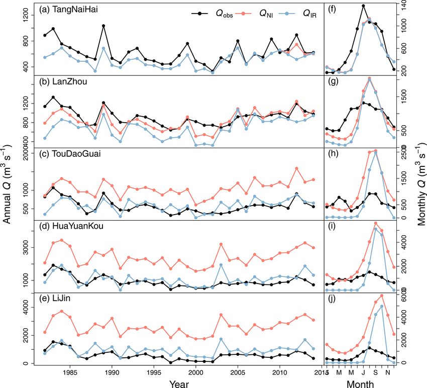
1134                                          Z. Yin et al.: Impacts of irrigation and damming on Yellow River streamflows

et al., 2018; Wada et al., 2014), these usages being influenced    and Tang et al. (2008). Yet, Jia et al. (2006) prescribed cen-
by direct anthropogenic drivers and by climate change (Had-        sus irrigation and dam operation data as input of their model.
deland et al., 2014; Piao et al., 2007, 2010; Yin et al., 2020;    Tang et al. (2008) included irrigation as a mechanism in
Zhou et al., 2020). In order to meet the fast-growing wa-          their DBH (distributed biosphere hydrological) model and
ter demand in populated areas and to control floods (Wada          investigated the long-term trends of streamflows, but they
et al., 2014), reservoirs have been built for regulating the       described the irrigation demand simply from satellite leaf
temporal distribution of river water (Biemans et al., 2011;        area data, so that crop plant water requirements and phenol-
Hanasaki et al., 2006), leading to a massive perturbation of       ogy were not represented by physical laws. Several global
the seasonality and year-to-year variations of streamflows. In     hydrological models (GHMs) simulated both irrigation and
the midlatitude–northern latitude regions, where a decrease        dam operation processes and were applied for future projec-
of rainfall is observed historically and projected by climate      tion of water resources regionally (Liu et al., 2019) or glob-
models (IPCC, 2014), water scarcity will be further exacer-        ally (Hanasaki et al., 2018; Wada et al., 2014, 2016). Those
bated by the growth of water demand (Hanasaki et al., 2013)        global GHM studies acknowledged the complex situation of
and by the occurrence of more frequent extreme droughts            the YRB where models’ performances are limited, but none
(Seneviratne et al., 2014; Sherwood and Fu, 2014; Zscheis-         has focused on the sources of error or potential overlooked
chler et al., 2018). Thus, adapting river management is a          mechanisms in this catchment.
crucial question for sustainable development, which requires          To model present water resources in the YRB and make
comprehensive understanding of the impacts of human ac-            future projections, not only natural mechanisms, but also an-
tivities on river flow dynamics„ particularly in regions under     thropogenic ones must be represented in a model. If a key
high water stress (Liu et al., 2017; Wada et al., 2016).           mechanism is missing in a model, a calibration of its pa-
   The Yellow River (YR) is the second longest river in            rameters to match observations can compensate for structural
China. It flows across arid, semi-arid, and semi-humid re-         biases, and projections may be erroneous. For example, the
gions, and the catchment contains intensive agricultural           HBV model (Hydrologiska Byråns Vattenbalansavdelning)
zones and has a population of 107 million inhabitants (Piao        was well calibrated with different approaches in 156 catch-
et al., 2010). With 2.6 % of total water resources in China, the   ments in Austria but failed in predicting streamflow changes
Yellow River basin (YRB) irrigates 9.7 % of the croplands          due to climate warming (Duethmann et al., 2020), one of the
(http://www.yrcc.gov.cn, last access: 28 February 2021). Un-       key reasons being that the response of vegetation to climate
derground water resources are used in the YRB, but they            change was missing in the model. In this study, we inte-
only account for 10.3 % of total water resources, outlining        grate two key anthropogenic processes (irrigation and dam
the importance of streamflow water for regional water use.         operation) in the land surface model ORCHIDEE (ORganiz-
A special feature of the YRB is the huge spatiotemporal            ing Carbon and Hydrology in Dynamic EcosystEms), which
variation of its water balance. Precipitation is concentrated      has a mechanistic description of plant–climate and soil wa-
in the flooding season (from July to October) which consti-        ter availability interactions and of river streamflows. Through
tutes ∼ 60 % of the annual discharge, whereas the dry season       a set of simulations with generic parameter values, we aim
(from March to June) represents only ∼ 10 %–20 %. Numer-           to preliminarily diagnose how irrigation and dam operation
ous dams have been built to regulate the streamflows intra-        improve the simulations of observed YRB streamflows. Af-
and inter-annually in order to control floods and alleviate wa-    ter making sure we understand the impact of adding these
ter scarcity (Liu et al., 2015; Zhuo et al., 2019). The YRB        two new and crucial processes, the model will be calibrated
streamflows are thus highly controlled by human water with-        against a suite of observations so that it can be applied for
drawals and dam operations, making it difficult to separate        future projections.
the impacts of human and natural factors on the variability           Using a standard version of ORCHIDEE without irrigation
and trends.                                                        or dams, Xi et al. (2018) performed simulations with a 0.1◦
   Numerous studies documented the effects of anthro-              hypo-resolution atmospheric forcing over China (Chen et al.,
pogenic factors on streamflows and water resources in the          2011). They attributed the trends of several river streamflows
YRB by statistical approaches (e.g., Liu and Zhang, 2002; Jin      to natural drivers from increased CO2 and climate change
et al., 2017; Miao et al., 2011; Wang et al., 2006, 2018; Zhuo     and to land use change. Lacking irrigation and other human
et al., 2019). To further elucidate the mechanisms, physical-      removals, their simulated results were higher than the ob-
based land surface hydrology models including natural and          served streamflows for the YRB. By developing a crop mod-
anthropogenic factors are required. Many previous model            ule in ORCHIDEE (Wang et al., 2016; Wang, 2016; Wu et al.,
studies only considered natural processes, and YRB simu-           2016), ORCHIDEE was able to provide precise estimation
lations were evaluated against naturalized streamflows (Liu        of crop physiology, phenology, and yield at both local and
et al., 2020; Xi et al., 2018; Yuan et al., 2018; Zhang and        national scales, as well as other site-based crop models, e.g.,
Yuan, 2020). YRB modeling studies simulating real stream-          EPICs (Folberth et al., 2012; Izaurralde et al., 2006; Liu et al.,
flows and comparing their values to observed streamflows           2007, 2016; Williams, 1995), CGMS-WOFOST (de Wit and
are scarce, the most important being from Jia et al. (2006)        van Diepen, 2008), APSIM (Elliott et al., 2014; Keating

Hydrol. Earth Syst. Sci., 25, 1133–1150, 2021                                       https://doi.org/10.5194/hess-25-1133-2021
Z. Yin et al.: Impacts of irrigation and damming on Yellow River streamflows                                                 1135

et al., 2003), and DSSAT (Jones et al., 2003), and land sur-       streams, which simplifies the assessment of the effects of ir-
face models, e.g., CLM-CROP (Drewniak et al., 2013), LPJ-          rigation and damming on streamflows.
GUESS (Smith et al., 2001; Lindeskog et al., 2013), LPJmL             In this study, ORCHIDEE, with the novel crop–irrigation
(Waha et al., 2012; Bondeau et al., 2007), and PEGASUS             module (Wang, 2016; Yin et al., 2020) and the new dam op-
(Deryng et al., 2011, 2014; Wang et al., 2017; Müller et al.,      eration model, was applied in the YRB from 1982 to 2014
2017). ORCHIDEE-estimated irrigation accounts for poten-           in order to (1) demonstrate whether ORCHIDEE and the
tial ecological and hydrological impacts (e.g., physiological      dam model, with generic parameterizations, are able to im-
response of plants to climate change and short-term drought        prove the simulation of streamflow fluctuations and (2) at-
episodes on soil hydrology) with respect to other land sur-        tempt to separate the effect of irrigation and dams on the fluc-
face models (LSMs) and GHMs (Hanasaki et al., 2008; Leng           tuations of monthly streamflows. We first describe the OR-
et al., 2015; Thiery et al., 2017; Nazemi and Wheater, 2015;       CHIDEE model and our new dam model in Sect 2.1. Then
Voisin et al., 2013). In a study focusing on China (Yin et al.,    we present the algorithm used for estimating sub-catchment
2020), ORCHIDEE was able to simulate irrigation with-              water balances in Sect. 2.2, followed by the input and evalu-
drawals across China and to evaluate them against census           ation datasets, the simulation protocol, and metrics for eval-
data with a provincial-based spatial correlations of ∼ 0.68.       uation in Sect. 2.3 to 2.5. Results are presented in Section 3,
It successfully explained the decline of total water storage       and limitations are discussed in Sect. 4.
in the YRB. In this study, we add a simple module describ-
ing the dam operations to further improve the model over the
YRB.                                                               2     Methodology
   A simple dam operation model is developed and firstly
coupled to ORCHIDEE to simulate the real streamflows in            2.1     ORCHIDEE land surface model used in this study
this study. Similar to other GHMs and LSMs, our dam oper-
ation model is based on generic operation principles due to a      2.1.1    Irrigation and crop modules
lack of related data. Recent dam models are developed from
different perspectives, such as the agent-based model River        ORCHIDEE is a physical process-based land surface model
Wave (Humphries et al., 2014), the basin-specific model            that integrates the hydrological cycle, surface energy bal-
Colorado River Simulation System (Bureau of Reclamation,           ances, the carbon cycle, and vegetation dynamics using
2012), and the original dam module in the Variable Infiltra-       two main modules. The SECHIBA (surface–vegetation–
tion Capacity (VIC) model (Lohmann et al., 1998). How-             atmosphere transfer scheme) module simulates the dynam-
ever, the representation of dam operations in many global          ics of the water cycle, energy fluxes, and photosynthesis at a
hydrological studies (e.g., Droppers et al., 2020; Haddeland       0.5 h time interval, which are used by the STOMATE (Saclay
et al., 2006, 2014; Hanasaki et al., 2018; Zhao et al., 2016;      Toulouse Orsay Model for the Analysis of Terrestrial Ecosys-
Yassin et al., 2019; Wada et al., 2014, 2016) is based on the      tems) to estimate vegetation and soil carbon cycle at daily
ideas of Hanasaki et al. (2006). They categorized dams based       time step. The ORCHIDEE model used in this study is a spe-
on their regulation purposes (irrigation and non-irrigation).      cial version with a newly developed crop and irrigation mod-
Irrigation-oriented rules adjust the dam retention to meet the     ule (Wang et al., 2017; Wu et al., 2016; Yin et al., 2020). The
irrigation demand downstream, while non-irrigation-oriented        crop module includes specific parameterizations for wheat,
rules buffer floods and thus dampen the variability (Hanasaki      maize, and rice, calibrated over China using observations
et al., 2006). However, the water release target of a dam in       (Wang, 2016; Wang et al., 2017). It is able to simulate crop
the model of Hanasaki et al. (2006) is fixed at the begin-         carbon allocation and different phenological stages, as well
ning of the year and cannot adjust interactively to large intra-   as related management (e.g., planting date, rotation, multi-
and inter-annual climate variations, which is a key feature        cropping, and irrigation).
of the YRB. To overcome this limitation, we propose a new             Irrigation amount is simulated in the land surface model
dam operation model based on a target operation plan, con-         ORCHIDEE (Wang, 2016; Wang et al., 2017) as the mini-
strained by the regulation capacity of a dam and historical        mum between crop water requirements and the water sup-
simulated streamflows, with flexibility to adjust to climate       ply. The crop water requirements are defined according to
variation. The effects of dams on streamflows could then be        the choice of irrigation technique, namely minimizing soil
studied with ORCHIDEE and isolated from the effect of cli-         moisture stress for the flooding technique, sustaining plant
mate factors and irrigation demands. Different from classical      potential evapotranspiration for the dripping technique, and
approaches separating the YRB into an upper, middle, and           maintaining the water level above the soil surface during spe-
lower stream (Tang et al., 2008; Zhuo et al., 2019), here we       cific months for the paddy irrigation technique. Each crop
further divide both the upper and middle streams into sub-         is grown on a specific soil column (in each model grid
catchments based on the locations of five key gauging sta-         cell), where the water and energy budgets are independently
tions (Fig. 1). This approach splits regions with and without      resolved. The water resources in the hydrological routing
big dams (or large irrigation areas) in the upper and middle       scheme are from three water reservoirs: (1) a streamflow

https://doi.org/10.5194/hess-25-1133-2021                                        Hydrol. Earth Syst. Sci., 25, 1133–1150, 2021
1136 Z. Yin et al.: Impacts of irrigation and damming on Yellow River streamflows
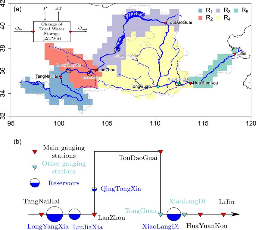
Figure 1. (a) Map of YRB. Gray and blue lines indicate the catchment and network of YR based on GIS data, respectively. Dark circles
are main artificial reservoirs on the YR. Triangles are gauging stations. Red triangles are main stations used for classifying sub-catchment
and simulation comparison, and teal triangles are stations used to assess the impacts of XiaoLangDi Reservoir on river streamflows. Colored
patterns are sub-catchments between two neighboring gauging stations based on the ORCHIDEE routing map. The water balances of specific
sub-catchments are shown in the top left. (b) Conceptual figure of YR main stream, gauging stations, and artificial reservoirs. The sizes of
circles indicate the regulation capacities of these reservoirs (Table 2).
component, (2) a fast reservoir with surface runoff, and (3) a mands. It has been developed for the main reservoirs of the
slow reservoir with deep drainage, used in this order for YRB (e.g., the LongYangXia, LiuJiaXia, and XiaoLangDi in
defining the priorities of water use for irrigation. As long- Fig. 1). Different from Biemans et al. (2011) and Hanasaki
distance water transfer is not modeled, streams only supply et al. (2006), we primarily consider the ability of reservoirs
water to the crops growing in the grid cell they cross, accord- to regulate river flow seasonality. This means that the target
ing to the river routing scheme of the ORCHIDEE model base flow and flood control of our dam model are not fixed
(Ngo-Duc et al., 2007). Without dams, irrigation can be un- proportions of the mean annual streamflow but depend on the
derestimated where dams store water to supply the crop de- regulation capacity of the reservoir (Cmax ). Firstly, similar to
mand. Transfer from reservoirs, lakes, or local ponds to ad- Voisin et al. (2013), a multi-year averaged monthly stream-
jacent cells is not considered, which should further lead to flow (Qs ) is calculated based on ORCHIDEE simulations.
an underestimation of the irrigation supply, dependent on the To include the potential impacts of recent climate change on
cell size. Details of the coupled crop–irrigation module of dam operation, here we only consider the latest past 10-year
ORCHIDEE are described in Yin et al. (2020). simulations, as
2.1.2 New dam operation model j ∈N
1 X j
Qs,i = Qi . (1)
N j
To account for the impacts of dam regulation on streamflow
(Q) seasonality, we developed a dynamic dam water stor-
age module based on only two generic rules: reducing flood Here Qs,i (m3 s−1 ) is the multi-year averaged monthly
peaks and guaranteeing base flow. This model depends on streamflow of month i; j is the year index; and N is the num-
simulated inflows and is thus independent from irrigation de- ber of years accounted for. For an upcoming year j , we only
Hydrol. Earth Syst. Sci., 25, 1133–1150, 2021 https://doi.org/10.5194/hess-25-1133-2021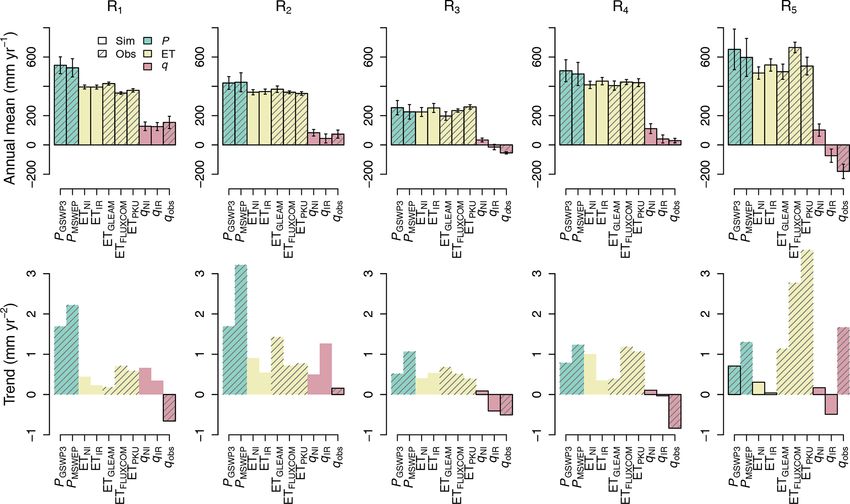
Z. Yin et al.: Impacts of irrigation and damming on Yellow River streamflows                                                                1137

use the historical simulations (maximum latest 10 years) to                      (Eq. 6), we decide to recharge additional water volume be-
calculate Qs .                                                                   sides the 1Wt,i .
   Secondly, we evaluate the target water storage change                            1W is then applied as a correction of simulated stream-
1Wt and monthly streamflow Qt considering the regulation                         flows to generate actual monthly streamflows using the fol-
capacity of each reservoir. As shown in Fig. S1 in the Supple-                   lowing equation:
ment, 1 year can be divided into two periods by comparing                                             1
Qs with Qs . The longest continuous period of months with                        Q̂sim,i = Qsim,i −     1Wi .                                 (7)
                                                                                                      α
Qs > Qs is the recharging season for reservoirs, and the rest
is the releasing season. The amount of water stored during                       Here Q̂sim (m3 s−1 ) is the simulated regulated streamflows,
the recharging season (blue region in Fig. S1) is determined                     and Qsim (m3 s−1 ) is the simulated monthly streamflows.
by Cmax and is used during the releasing season (red regions                     Note that this model is a simplified representation of dam
in Fig. S1). The values of 1Wt and Qt can be estimated by                        management because it ignores the direct coupling between
                                                                                 water demand and irrigation water supply from the cascade
               Cmax
                                                                                 of upstream reservoirs. This approach implies that, with a
k = min                      , kmax ,                      (2)
             i∈Recharge
                X                                                                regulated flow, demands will be able to be satisfied and floods
           α            Qs,i                                                     avoided without being more explicit. A complete coupling
                    i
                                                                              of demand, flood, and reservoir management is difficult to
1Wt,i     = α k Qs,i − Qs + Qs ,                                           (3)   implement in the land surface model in the absence of data
Qt,i = Qs,i − 1Wt,i /α.                                                    (4)   about the purpose and management strategy of each dam,
                                                                                 given different possibly conflicting demands of water for in-
Here k (–), varying between 0 and kmax (= 0.7), indicates the                    dustry and drinking versus cropland irrigation.
ability of the reservoir to disturb streamflow seasonality. It                      Before performing the simulation, we estimate the max-
is a ratio of the maximum regulation capacity of the reser-                      imum regulation capacity of each studied reservoir in each
voir Cmax (108 m3 ) over the streamflow amount throughout                        river sub-catchment shown in Fig. 1. Table 1 lists collected
the recharging season. α (0.0263) converts monthly stream-                       information of the main reservoirs on the YR. Only large
flow to water volume. Assuming that the water storage of the                     reservoirs like LongYangXia (LYX), LiuJiaXia (LJX), and
reservoir reaches Cmax at the end of the recharging season,                      XiaoLangDi (XLD) are considered in our model because of
we can calculate target water storage Wt by using 1Wt .                          their huge Cmax .
   Finally, the variation of the actual water storage of the
reservoir 1W is a decision regarding actual monthly stream-                      2.2   Sub-catchment diagnosis
flow, current water storage, Qt , 1Wt , and Wt . During the re-
leasing season, 1W is calculated as                                              Figure 1 shows the YRB and main gauging stations used in
                                                                                 this study. To effectively use Qobs for investigating impacts
 −Wi ( Wt,i t,i )
       −1W
                                         if Wi ≤ Wt,i ;                          of irrigation and dam regulations on the streamflows of dif-
                                                                           (5)
        h                         i
 1W̃i −    Wi + 1W̃i − Wt,i + 1Wt,i      if Wi > Wt,i and 1W̃i > 1Wt,i ;         ferent river sub-catchments, we divided the YRB into five

 1Wt,i − Wi − Wt,i                       if Wi > Wt,i and 1W̃i ≤ 1Wt,i .
                                                                                 sub-catchments (Ri , i ∈ [1, 5]; Fig. 1) with an outlet at each
1W̃i = αQi − (αQt,i − 1Wt,i ). It is the expected release                        gauging station. Thus we can evaluate the water balance in
amount to make river streamflows equal to the target stream-                     Ri by
flows after reservoir regulation. If current water storage is                    1TWSi              Qin,i − Qout,i
                                                                                       = Pi − ETi +                ,                          (8)
less than the target value (the case of Eq. 5), the 1Wi is cal-                   1t                      Ai
culated by the Wi with a proportion of 1Wt,i over Wt,i . If
                                                                                 where 1t is the time interval, 1TWSi (mm) is the change of
the current storage is more than the target value (the cases of
                                                                                 total water storage in specific Ri , Pi (mm 1t −1 ) is precipita-
Eq. 5), the reservoir can release more water based on a bal-
                                                                                 tion in Ri , ETi (mm 1t −1 ) is evapotranspiration in Ri , and
ance between the target water storage change 1Wt,i and the
                                                                                 Ai (m2 ) is the area of Ri . Qin,i and Qout,i (m3 1t −1 ) are in-
target water storage at the next time step Wt,i (represented
                                                                                 flow and outflow respectively. In addition, qi = Qout,i −Qin,i
by 1W̃i ). Note that all water storage change variables are
                                                                                 indicates the contribution of Ri to the river streamflows, that
negative throughout the releasing season.
                                                                                 is the sub-catchment streamflows. This term can be negative
   During the recharging season, we can calculate the 1Wi
                                                                                 if local water supply (e.g., precipitation and groundwater)
as
                                                                               cannot meet water demand. A conceptual figure of the water
  max min Wt,i + 1Wt,i − Wi , αQ i , 0 if Wi > Wt,i ; (6)                      balance of a sub-catchment is shown in the top left of Fig. 1.
  min 1Wt,i + Wt,i − Wi , αQi               if Wi ≤ Wt,i .
                                                                                 2.3   Evaluation datasets
If current water storage is larger than the target value (Eq. 6),
we will try to recharge a volume of water to make Wi+1 =                         Observed monthly streamflows (Qobs ) from the gauging
Wt,i+1 . If current water storage is less than the target value                  stations shown in Fig. 1 are used to evaluate the simula-

https://doi.org/10.5194/hess-25-1133-2021                                                     Hydrol. Earth Syst. Sci., 25, 1133–1150, 2021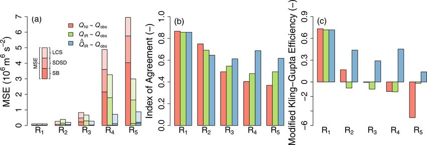
1138                                                     Z. Yin et al.: Impacts of irrigation and damming on Yellow River streamflows

Table 1. Information of artificial reservoirs on the YR with considerable total capacity. Data are mainly from the YR Conservancy Commis-
sion of the Ministry of Water Resources (http://www.yrcc.gov.cn, last access: 28 February 2021). The “regulation purposes” follow the style
of Hanasaki et al. (2006). “H” indicates hydropower; “C” indicates flood control; “I” indicates irrigation; “W” indicates water supply; and
“S” indicates scouring sediment.

   Name                  Total capacity (108 m3 )      Regulation capacity (108 m3 )   Regulation since   Regulation type   Regulation purposes
   LongYangXia                                 247                           193.53    Oct 1986           Inter-annual      HCIW
   LiJiaXia                                   16.5                                –    Dec 1996           Daily, weekly     HI
   GongBoXia                                    6.2                            0.75    Aug 2004           Daily             HCIW
   LiuJiaXia                                     57                            41.5    Oct 1968           Inter-annual      HCIW
   YanGuoXia                                   2.2                                –    Mar 1961           Daily             HI
   BaPanXia                                   0.49                             0.09    –                  Daily             HIW
   QingTongXia                         6.06 → 0.4∗                                –    1968               Daily             HI
   XiaoLangDi                                126.5                             91.5    1999               Inter-annual      CSWIH
∗ The total capacity shrink is due to sedimentation.

tions. Several precipitation (P ) and evapotranspiration (ET)                    to the modeled crop (wheat, maize, and rice) is used, based
datasets were selected to evaluate the simulated water bud-                      on a 1 : 1 million vegetation map and provincial-scale cen-
gets in each sub-catchment of the YRB. The 0.5◦ 3-hourly                         sus data of China. Crop planting dates for wheat, maize, and
precipitation data from GSWP3 (Global Soil Wetness Project                       rice are derived from the spatial interpolation of phenolog-
Phase 3) used as model input are based on GPCC v6 (Global                        ical observations from the Chinese Meteorological Admin-
Precipitation Climatology Centre; Becker et al., 2013) af-                       istration (Wang et al., 2017). The soil texture map is from
ter bias correction with observations. The MSWEP (Multi-                         Zobler (1986). Two simulation experiments were performed
Source Weighted-Ensemble Precipitation) is a 0.25◦ 3-hourly                      to assess the impacts of irrigation on streamflows: (1) NI, no
P product integrating numerous in situ measurements, satel-                      irrigation, and (2) IR, irrigated by available water resources.
lite observations, and meteorological reanalysis (Beck et al.,                   In IR, only surface irrigation is considered, that is, water ap-
2017). Three ET datasets are chosen for their potential abil-                    plied on the cropland soil without interception by canopies.
ity to capture the effect of irrigation disturbance on ET (Yin                   The soil water stress, a function of soil moisture and crop root
et al., 2020) (noted as ETobs ). GLEAM v3.2a (Global Land                        density up to 2 m depth (Yin et al., 2020), is checked every
Evaporation Amsterdam Model; Martens et al., 2017) pro-                          half an hour. When it is less than a target threshold, irrigation
vides 0.25◦ daily ET estimations based on a two-soil layer                       is triggered with an amount equal to the difference between
model in which the top soil moisture is constrained by the                       saturated and current soil moisture. To precisely estimate ir-
ESA CCI (European Space Agency Climate Change Ini-                               rigation water consumption (direct water loss from the sur-
tiative) Soil Moisture observations. The FLUXCOM model                           face water pool excluding return flow), deep drainage of the
(Jung et al., 2009) upscales ET data from a global network                       three crop soil columns is turned off in the IR simulation.
of eddy covariance tower measurements into a global 0.5◦                         Simulations start from a 20-year spin-up in 1982 to initialize
monthly ET product. Since these towers do not cover irri-                        the thermal and hydrological variables then continued from
gated systems, ET from irrigation simulated by the LPJmL                         1982 to 2014. A validation against naturalized streamflows is
(Lund–Postam–Jena managed Land) is added to ET from                              shown in the Supplement Table S1.
non-irrigated systems. The PKU ET product estimates 0.5◦                            The dam operation simulation starts from 1982 as an of-
monthly ET using water balances at basin scale, integrating                      fline model applied to the simulated streamflows from the IR
FLUXNET observations to diagnose sub-basin patterns us-                          simulation (QIR ) as input. The initial values of W were set
ing a model tree ensemble approach (Zeng et al., 2014).                          to half of the Cmax . Considering the potential joint regulation
                                                                                 of reservoirs, we firstly estimate the total 1W of all consid-
2.4     Simulation protocol                                                      ered reservoirs by using QIR at HuaYuanKou (outlet of R4 ;
                                                                                 Fig. 1). Then we estimate the 1W of LYX and LJX reservoir
The 0.5◦ half-hourly GSWP3 atmospheric forcing (Kim,                             by using QIR at LanZhou. The difference between these two
2017) was used to drive ORCHIDEE simulations. Yin et al.                         1W is assumed to be the 1W of the XLD reservoir in be-
(2018) used four atmospheric forcing datasets to drive OR-                       tween. Offline simulated 1W values are used to estimate reg-
CHIDEE to simulate soil moisture dynamics over China, and                        ulated monthly streamflows (Q̂IR ) as in Eq. (7). As huge irri-
they found that the GSWP3 provided the best performances;                        gation water withdrawals occur in R3 and R5 (YRCC, 2014),
hence we chose this forcing for this study. A 0.5◦ map with                      the water recharge of reservoirs may result in negative Q̂IR at
15 different plant functional types (PFTs) containing crop                       TouDaoGuai and LiJin. To avoid this numerical artifact due
sowing area information for the three PFTs corresponding                         to the offline nature of our dam model, we corrected all neg-

Hydrol. Earth Syst. Sci., 25, 1133–1150, 2021                                                      https://doi.org/10.5194/hess-25-1133-2021
Z. Yin et al.: Impacts of irrigation and damming on Yellow River streamflows 1139
Table 2. Definitions of sub-catchments and values of Cdam used in The modified Kling–Gupta efficiency (mKGE ∈ (−∞, 1])
the dam regulation simulation. is defined as the Euclidean distance of three independent cri-
teria: correlation coefficient r, bias ratio β, and variability
Sub-catchment Stations Cdam (108 m3 ) Regulation ratio γ (Gupta et al., 2009; Kling et al., 2012). It is an im-
since proved indicator from the Nash–Sutcliffe efficiency avoiding
– heterogeneous sensitivities to peak and low flows, which is
R1 – –
TangNaiHai crucial for this study that is not only interested in simulating
TangNaiHai 41.5 before 1987; peak flows but also concentrates on base flows regulated by
R2 1982 dams for human usage. The mKGE is calculated as
LanZhou 235 after 1987
LanZhou q
R3 – 1982
TouDaoGuai mKGE = 1 − (1 − r)2 + (1 − β)2 + (1 − γ )2 , (11)
R4
TouDaoGuai
91.5 1999
µS CVS
HuaYuanKou β= ;γ = , (12)
µO CVO
HuaYuanKou
R5 – – where r is the correlation coefficient between observed and
LiJin
simulated streamflows, and µ (m3 s−1 ) and CV (–) are the
mean and the coefficient of variation of Q, respectively.
ative Q̂IR to zero by assuming that the streamflows cannot These indicators are used for three comparisons: (1) QNI and
further drop when all stream water is consumed upstream. Qobs , (2) QIR and Qobs , and (3) Q̂IR and Qobs .
The impact of these corrections is accounted for at gauging
stations downstream to ensure mass conversation.
3 Results
2.5 Evaluation metrics
3.1 Water budgets at sub-catchment scale
Three metrics are used to evaluate the performances of simu-
lated monthly Q. The mean square error (MSE) evaluates the Figure 2 displays water budgets and trends in Ri based
magnitude of errors between simulation and observations. It on simulation and observations. Going from upstream to
can be decomposed into three components (Kobayashi and downstream, precipitation in PGSWP3 , which is consis-
Salam, 2000): tent with PMSWEP , decreases from 543.6 mm yr−1 (R1 ) to
254.2 mm yr−1 (R3 ) and then rises again to 652.1 mm yr−1
n (R5 ). The magnitudes of simulated ET (both ETNI and ETIR )
1X
MSE = (Si − Oi )2 = SB + SDSD + LCS, (9) have no significant differences with ETobs aggregated over
n i=1
sub-catchments R1 to R5 . Grid-cell-based validation shows
where Si and Oi are simulated and observed values, respec- high agreement between simulated and observed ET across
tively, and n is the number of samples. SB (squared bias) all sub-catchments. The lowest mean of correlation coeffi-
is the bias between simulated and observed values. In this cients is 0.79, and the highest mean of relative root mean
study, SB represents the difference between simulated and square error (RMSE) is 4.9 % (Table S2). Except for R1
observed multi-year mean annual Q. SDSD (the squared dif- where cropland is rare, ETIR accounts for an amount rep-
ference between standard deviation) relates to the mismatch resenting more than 80 % of PGSWP3 in the YRB, with a
of variation amplitudes between simulated and measured val- maximum value of 96.5 % in R3 . The difference between
ues. It can reflect whether our simulation can capture the ETIR and ETNI is due to the irrigation process, which ac-
seasonality of Qobs . LCS (the lack of correlation weighted counts for 9.1 % and 8.2 % of ETNI in R3 and R5 respec-
by the standard deviation) indicates the mismatch of fluctua- tively as caused by the irrigation demand. The impact of
tion patterns between simulated and observed values, which irrigation can be detected from sub-catchment streamflows
is equivalent to inter-annual variation of Q in this study. The (qi = (Qout,i − Qin,i )/Ai ) as well. For instance, both qobs
formulas of these three components and a detailed explana- and qIR are negative in R3 and R5 , suggesting that local sur-
tion can be found in Kobayashi and Salam (2000). face water resources cannot meet water demand for irriga-
The index of agreement (d ∈ [0, 1]) is defined as the ratio tion. As irrigation water transfers between grid cells are not
of MSE and potential error. It is calculated as represented in our simulations, the non-availability of water
Pn locally results in an underestimation of the irrigation with-
2
i=1 (Oi − Si ) drawals, likely explaining why qIR > qobs in R3 to R5 .
d = 1− P 2 , (10)
n The trends of P and ET are positive but not significant
i=1 |Si − O| + |Oi − O|
in most Ri during the period 1982–2014 (bottom panels of
where d = 1 indicates perfect fit, and d = 0 denotes poor Fig. 2). However, significant trends can be found in simu-
agreement. lated and observed q in some Ri . The decrease of qobs in R1
https://doi.org/10.5194/hess-25-1133-2021 Hydrol. Earth Syst. Sci., 25, 1133–1150, 20211140 Z. Yin et al.: Impacts of irrigation and damming on Yellow River streamflows
Figure 2. Top panels: annual mean of hydrological elements in each sub-catchment of the YR basin from both simulation (plain colors) and
observation (hatched colors). Error bars represent standard deviation. Bottom panels: trends of these elements in each sub-catchment. Dark
borders indicate the trend is statistically significant (p-value < 0.05) according to the Mann–Kendall test.
is not captured by the model, neither in qNI nor qIR . This un- is lower, and a larger fraction of P can go to runoff. This
derestimated decrease of river streamflows might be linked mechanism highlighted that irrigation could enhance the het-
to decreased glacier melt or increased non-irrigation-related erogeneity of water temporal distribution and may reinforce
human water withdrawals, which are ignored in our simula- floods after a dry season.
tions. In R2 and R3 , the qobs trends are determined by the
joint effects of climate change (e.g., the P increase) and hu- 3.2 Comparison between observed and simulated Q
man water withdrawals. The trends of qIR show the same di-
rection as those of qobs . In R5 , however, qobs increased by Figure 3 shows time series of annual streamflows and of the
1.67 mm yr−1 , which was not captured by our simulation of seasonality of monthly streamflows. Our simulations under-
qIR . Besides the increase of P , another possible driver of in- estimate Qobs at TangNaiHai in R1 , likely because we miss
creasing qobs in R5 is a decrease of water withdrawal due to glacier melt. After LanZhou, the values of QIR coincide very
the improvement of irrigation efficiency (Yin et al., 2020), well with those of Qobs , indicating that irrigation strongly
which is not accounted for in our simulations. Moreover, wa- reduces the annual streamflows of the YR. However, the sea-
ter use management may play an important role in the ob- sonality of monthly QIR is different from Qobs (Fig. 3f–j).
served positive trends of qobs as well, with the aim to increase Despite the good match of annual values, the model with-
the streamflows downstream of the YR to avoid streamflow out dams (shown in Fig. 3) produces an underestimation of
cutoff (Qobs < 1 m3 s−1 ) that occurred in the 1990s (Wang Q in the dry season and an overestimation of Q in the flood
et al., 2006). season. Such a mismatch of Q seasonality is likely caused
Irrigation not only influences annual streamflows in the primarily by dam regulation ignored in the model. The loca-
YR but also affects its intra-annual variation. In general, the tions of several big reservoirs are shown in Fig. 1b, and their
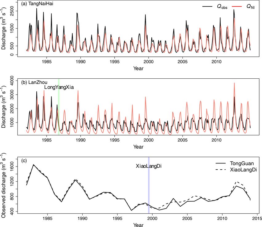
discharge yield YQ , defined by the sum of surface runoff characteristics are listed in Table 1.
and drainage, of all grid cells in NI should be higher than in Regarding dams, before the operation of the LongYangXia
IR because our irrigation model can remove water from the dam in 1986, which brought a regulation capacity of 193.5 ×
stream reservoirs which is a fraction of drainage and runoff. 108 m3 (green bar in Fig. 4b), the peaks of monthly QNI at
However, our simulations show that YQ,NI can be less than LanZhou were slightly lower than the peaks of Qobs in R2
YQ,IR (Fig. S2) at the beginning of the monsoon season. This (Fig. 4b), as well as at TangNaiHai (Fig. 4a). But after the
is because irrigation keeps soil moisture higher than with- construction of the LongYangXia dam, modeled peak QNI
out irrigation in July in R4 and R5 (Fig. S2d and e), which became systematically higher than the peak of Qobs each
in turn promotes YQ because the soil water-holding capacity year, suggesting that the construction of this dam caused the
observed peak reduction (Fig. 4b). Moreover, the seasonality
Hydrol. Earth Syst. Sci., 25, 1133–1150, 2021 https://doi.org/10.5194/hess-25-1133-2021Z. Yin et al.: Impacts of irrigation and damming on Yellow River streamflows 1141
Figure 3. (a–e) Time series of annual streamflows from observations and simulations at each gauging station. (f–j) Seasonality of observed
and simulated streamflows at each gauging station. Qobs is the observed annual mean streamflows. QNI and QIR are the simulated annual
mean streamflows based on the NI and IR simulations (Sect. 2.4), respectively. These simulations do not account for dams, and therefore the
seasonality has a higher amplitude than observed in the plots on the right-hand side.
of Qobs changed dramatically in the period (1982–2014), but The dam model is successful in reproducing flood control
no similar trend was found in monthly P (Fig. S3), suggest- as well. At LanZhou, although Q̂IR underestimates the peak
ing that dam operation was the primary driver of the observed flow due to the bias of the simulated mean annual stream-
shift in seasonal streamflow variations of the YRB from 1982 flows (Fig. 3b), its seasonality is much smoother than that of
to 2014. Dams can affect inter-annual variations of Q as well, QIR . The underestimation of Q̂IR can reflect special water
although less than the seasonal variation. For instance, Tong- management during extreme years. From 2000 to 2002, the
Guan and XiaoLangDi are two consecutive gauging stations YRB experienced severe droughts, with 10 %–15 % precip-
upstream and downstream of the reservoir of XiaoLangDi itation less than usual, leading to a decrease of surface wa-
in R4 (Fig. 1). The annual Qobs at the two stations shows ter resources by as much as 45 % (Water Resources Bulletin
different features after the construction of the XiaoLangDi of China; http://www.mwr.gov.cn/sj/tjgb/szygb/, last access:
reservoir in 1999. 28 February 2021). To guarantee base flow, a set of policies
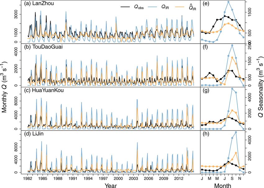
Figure 5 shows monthly time series of Qobs , QIR , and Q̂IR were applied (e.g., reducing water withdrawn, increasing wa-
(see Sect. 2.1.2) at each gauging station. Discharge fluctua- ter price, and releasing more water from reservoirs). These
tions are successfully improved in Q̂IR . Especially the base policies are not accounted for in the model, which will pro-
flow of Q̂IR coincides well with that of Qobs during win- duce a higher irrigation demand during dry years and pro-
ter and spring. The only exception occurs at LiJin, where mote the underestimation of the Qobs . From TouDaoGuai
Q̂IR overestimates the streamflows from January to May. In to LiJin, the floods from August to October are dramati-
fact, the water release from XLD during this period would cally reduced by our dam model. Nevertheless, the peaks
be withdrawn for irrigation and industry in R5 . However, our are still overestimated in Q̂IR , which might be due to numer-
offline dam model is not able to simulate the interactions, ous non-modeled medium/small reservoirs that were ignored
leading to the overestimation. by our model; no fewer than 203 medium reservoirs were
documented at the end of 2014 (YRCC, 2014). In our sim-
https://doi.org/10.5194/hess-25-1133-2021 Hydrol. Earth Syst. Sci., 25, 1133–1150, 20211142 Z. Yin et al.: Impacts of irrigation and damming on Yellow River streamflows Figure 4. (a–b) Monthly observed (Qobs ) and simulated (QNI ) streamflows at TangNaiHai and LanZhou stations. Green bar in (b) indicates the start of the LongYangXia dam regulation. (c) Observed annual streamflows at TongGuan and XiaoLangDi gauging stations, which are located up- and downstream of the XiaoLangDi reservoir, respectively (see Fig. 1). Blue bar in (c) indicates the start of the XiaoLangDi dam regulation. ulation, a 326.5 ×10⁸ m3 regulation capacity is considered, ment flushing downstream (Baoligao et al., 2016; Kong et al., which only accounts for 45 % of the total storage capacity of 2017; Zhuo et al., 2019), a process not represented in our 720 ×108 m3 (Ran and Lu, 2012). Moreover, in the five irri- simple dam model. Moreover, because we ignored the buffer- gation districts (http://www.yrcc.gov.cn/hhyl/yhgq/, last ac- ing effect of numerous medium reservoirs, the simulated wa- cess: 28 February 2021; Tang et al., 2008), special irrigation ter recharge during the flood season could be overestimated. systems in the YRB could contribute to flood reduction. For Figure 7 presents the model performances with differ- instance, the Hetao Plateau is the traditional irrigation district ent metrics in different Ri . The results show that MSE in- and is equipped with a hydraulic system that can divert river creases considerably from R1 to R5 , implying accumulated water into a complex irrigation network (bounded by 106.5– impacts of error sources in increasing the error of modeled Q 109◦ E and 40.5–41.5◦ N, shown in Fig. 1), by adjusting wa- when going downstream in the entire catchment. Most likely, ter level differences during the flood season. This no-dam those error sources are omission errors of anthropogenic fac- diversion system of the Hetao Plateau can take 50 ×108 m3 tors such as drinking and industrial water removals, but also as an extra regulation capacity per year, equivalent to 14 % of natural factors such as riparian wetlands and floodplains of the annual streamflow in R3 . (e.g., the SanShengGong water conservancy hub) and non- Simulated 1W in R2 is compared to observations (Jin represented small streams in the routing of ORCHIDEE (e.g., et al., 2017) in the left panel of Fig. 6, and the good agree- the irrigation system at the Hetao Plateau). From the de- ment suggests that our dam model is able to capture the sea- composition of MSE, we found that adding irrigation to the sonal variation of 1W (r = 0.9, p < 0.001) and rectify the model removes most of the bias in the average magnitude simulated streamflows. In the case of XiaoLangDi in the right Q by reducing the SB bias error term of the MSE. The only panel of Fig. 6, where the correlation is smaller (r = 0.34, exception occurs at LanZhou, where SB increases in IR, con- p = 0.28), the mismatch could be explained by sediment sequently leading to higher MSE. This misfit is due to the un- regulation procedures of that dam, given that it releases a derestimation of Q upstream (Fig. 3a). Thus, modeled QIR huge amount of water in June for reservoir cleaning and sedi- is lower at LanZhou, which enlarges the SB. On the other Hydrol. Earth Syst. Sci., 25, 1133–1150, 2021 https://doi.org/10.5194/hess-25-1133-2021
Z. Yin et al.: Impacts of irrigation and damming on Yellow River streamflows                                                         1143

Figure 5. Comparison between observed and simulated actual monthly streamflows at gauging stations. Qobs (dark lines) is observed monthly
streamflows. QIR (blue lines) is simulated monthly streamflows from the IR experiment (Sect. 2.4). Q̂IR (orange lines) is simulated monthly
streamflows including impacts of dam regulation (Sect. 2.4).

                                                                        man effects on Q of the YR were modeled brings more real-
                                                                        istic results, despite ignoring the direct effect of irrigation de-
                                                                        mand on reservoir release and ignoring industrial and domes-
                                                                        tic water demands. The mKGE reveals a significant increase
                                                                        after considering dam operations (Fig. 7c). Particularly at
                                                                        LanZhou and HuaYuanKou, the mKGE of Q̂IR ∼ Qobs in-
                                                                        creases by 0.86 and 1.11 compared to QIR ∼ Qobs , respec-
                                                                        tively. Note that the mKGEs of QIR ∼ Qobs are smaller than
                                                                        those of QNI ∼ Qobs from R2 to R4 because irrigation de-
                                                                        creases the mean annual streamflow of QIR , which further
                                                                        increases the CVS , leading to worse γ in mKGE (Eq. 11).
Figure 6. The changes of water storage of dams (1W ) in R2 and
R4 . The dark line represents the 1W from literature. The multi-
year mean of 1W of LongYangXia and LiuJiaXia is from Jin et al.
(2017). The 1W of XiaoLangDi is from the 1-year record reported         4   Discussion
in Kong et al. (2017). Red lines represent corresponding simulated
1W from our dam regulation model.                                       This study shows that ORCHIDEE land surface model with
                                                                        crops, irrigation, and our simple dam operation model can
                                                                        reproduce streamflow mean levels, inter-annual variations,
hand, adding the dam operation contributes to improve the               and the seasonal cycle in different sub-catchments of the
phase variations of Q which are dominated by the phase of               YRB correctly. We preliminarily quantified the impacts of
the seasonal cycle, by reducing the SDSD error term. Never-             irrigation and dams on the fluctuations of streamflows. Sim-
theless, the LCS error term, indicating the magnitude of the            ulated water balance components were compared to obser-
variability, mainly at inter-annual timescales, has no signif-          vations in different sub-catchments with a good agreement
icant improvement with the representation of irrigation and             (e.g., 4.5 ± 6.9% for ET). We found that irrigation mainly
dam regulations. It is because some of reservoirs are able to           affects the magnitude of annual streamflows by consuming
regulate Q inter-annually (Table 1), which can be observed              242.8 ± 27.8 × 10⁸ m3 yr−1 of water, consistent with cen-
from Fig. 4c. However, related operation rules are unclear              sus data giving a consumption of 231.4 ± 31.6 × 10⁸ m3 yr−1
and are not implemented in our dam model. Improvements                  (YRCC, 2014). As the water of the YRB is reaching the
were found in d as well, which demonstrates that the way hu-            limit of usage (Feng et al., 2016), we did not find any sig-

https://doi.org/10.5194/hess-25-1133-2021                                             Hydrol. Earth Syst. Sci., 25, 1133–1150, 2021
1144 Z. Yin et al.: Impacts of irrigation and damming on Yellow River streamflows Figure 7. Indicators of Q comparisons in each sub-catchment of the YRB. Colors indicate different comparisons. The MSE is decomposed to SB, SDSD, and LCS, which are distinguished by different transparencies. nificant effect of irrigation on streamflow trends. Instead of ing demands for water (e.g., policies, electricity price, water increasing river water withdrawals, the growing water de- price, land use change, irrigation techniques, water manage- mand appeared to have been balanced by improving wa- ment techniques, and dams inter-connection), which are dif- ter use efficiency during the study period (Yin et al., 2020; ficult to model well due to a lack of data. However, with the Zhou et al., 2020). Our simulation reveals that the impact of upcoming Surface Water and Ocean Topography (SWOT) irrigation on streamflows may even be positive under spe- mission, it will be possible to monitor the water level and cial situations, which was also shown in Kustu et al. (2011). surface extent of more reservoirs, which will be helpful to However, our mechanisms are different from the irrigation– improve and validate the dam operation simulations (Ottlé ET–precipitation atmospheric feedback mechanisms found et al., 2020). by Kustu et al. (2011); we demonstrated that irrigation may Our simulations ignored potential impacts of reservoirs significantly increase soil moisture and promote runoff yield on local climate, e.g., through their evaporation (Degu during the following wet season. It implies that irrigation in et al., 2011). The water area of several artificial reservoirs such landscapes may reinforce the magnitude of floods dur- (LongYangXia, LiuJiaXia, BoHaiWan, SanShengGong, and ing the rainy season by a higher legacy soil moisture. XiaoLangDi) is approximately 1056 km2 , which is larger We found that dams strongly regulate the temporal varia- than the 10th largest natural lake in China. These water tion of streamflows (Chen et al., 2016; Li et al., 2016; Yagh- bodies can also significantly influence local energy budgets, maei et al., 2018). By including simple regulation rules de- and evaporative water loss may be considerable, especially pending on inflows, our dam model reduced the simulation in arid and semi-arid areas (Friedrich et al., 2018; Shiklo- error by 48 %–77 % (MSE in Fig. 7), especially the variabil- manov, 1999). In addition, the five large irrigation districts ity component (SDSD) of the total error, which is dominated (http://www.yrcc.gov.cn/hhyl/yhgq/, last access: 27 Febru- by seasonal misfit reduction from dams. Moreover, we con- ary 2021) could dramatically alter the local climate through firmed that the change of Qobs seasonality during the study atmospheric feedbacks. For instance, the Hetao Plateau can period is not due to climate change (Fig. S3) but is deter- take about 50 ×108 m3 from streamflows every year during mined by dam operations (Wang et al., 2006). Big dams, like the flood season. Its irrigation area is 5740 km2 , with an evap- the LongYangXia, LiuJiaXia, and XiaoLangDi, are able to otranspiration rate ranging between 1200–1600 mm yr−1 . regulate streamflows inter-annually (Wang et al., 2018) and However, as these irrigation districts divert river water with- smooth the inter-annual distribution of water resources in the out big dams, they are not taken into account in most YR YRB (Piao et al., 2010; Wang et al., 2006; YRCC, 2014). studies. Another non-negligible factor in the case of YR is However, their detailed operation rules are unclear and were sedimentation, which reduces the regulation capacities of not implemented explicitly in our dam model. The error cor- reservoirs and weakens streamflow regulation by humans. responding to inter-annual variation (LCS in MSE in Fig. 7) For instance, the total capacity of QingTongXia has declined was thus not reduced by including dams. In the dam model, from 6.06 to 0.4 × 10⁸ m3 since 1978 due to sedimentation. some functions of reservoirs, such as providing irrigation Therefore, how land use change and the evolution of natural supply, industrial and domestic water, electricity generation, ecosystems affect sediment load and deposition is another and flood control (Basheer and Elagib, 2018), are not explic- key factor to project dams’ disturbances on streamflows in itly represented. Particularly the XiaoLangDi dam carries a the YRB. distinctive water-sediment mission, which scours sediments Simulating anthropogenic impact on river streamflows is downstream by creating artificial floods in June (Kong et al., challenging. In the case of the YR, well-calibrated mod- 2017; Zhuo et al., 2019). These functions are associated with els can provide accurate naturalized streamflow simulations, many socioeconomic factors and drivers, leading to compet- with Nash–Sutcliffe efficiency (NSE) as high as 0.9 (Yuan Hydrol. Earth Syst. Sci., 25, 1133–1150, 2021 https://doi.org/10.5194/hess-25-1133-2021
Z. Yin et al.: Impacts of irrigation and damming on Yellow River streamflows                                                     1145

et al., 2016). However, when considering the impacts of irri-     5   Conclusions
gation and dams, the NSE values of simulations are generally
worse. For instance, simulations with anthropogenic effects
by Hanasaki et al. (2018) had lower NSE than the simulation       A land surface model ORCHIDEE and a newly developed
with only natural processes. Similarly, Wada et al. (2014)        dam model are utilized to simulate the streamflow fluctu-
showed NSE decrease after considering anthropogenic fac-          ations and dam operations in the Yellow River basin. The
tors in the YRB, which was interpreted as complexity of           impacts of irrigation and dam regulation on streamflow fluc-
the YRB under the impacts of human activities and climate         tuations of the Yellow River were preliminarily qualified and
variation. However, the NSE of naturalized streamflows can-       quantified in this study by using a process-based land surface
not really be compared to the one of regulated streamflows.       model and a dam operation model. Irrigation mainly con-
Even if a model can perfectly simulate the dam operations,        tributes to the reduction of annual streamflow by as much as
the NSE of naturalized streamflows will be larger than that       242.8 ± 27.8 × 10⁸ m3 yr−1 . The shifts of intra-annual varia-
of regulated streamflows, given that dam operations auto-         tion of the Yellow River streamflows appear not to be caused
matically reduce the variation of river streamflows (a simple     by climate change, at least not by significant changes of pre-
proof is available in Sect. A of the Supplement). In fact, our    cipitation patterns and land use during the study period, but
model performances are very similar to GHM simulations            by the construction of dams and their operation. After consid-
(Fig. S2 from Liu et al., 2019). By gradually considering an-     ering the impacts of dams, we found that dam regulation can
thropogenic factors (irrigation and dam operations), the per-     explain about 48 %–77 % of the fluctuations of streamflows.
formances of our simulations increase dramatically accord-        The effect of dams may be still underestimated because we
ing to all three metrics.                                         only considered simple regulation rules based on inflows
   Intensive calibrations using a suite of observations can al-   but ignored its interactions with irrigation demand down-
low catchment-scale studies to provide highly accurate sim-       stream. Moreover, our analysis showed that several reservoirs
ulated streamflows for short-term flood forecasts. However,       on the Yellow River are able to influence streamflows inter-
for long-term projections, a model should include all key         annually. However, such effects are not quantified due to a
processes of the system studied. If key processes are miss-       lack of knowledge of the regulation rules across our study
ing in the model, a calibration will cover up the shortcom-       period.
ings, which lead to a lack of predictive capacities for long
timescales, as shown by Duethmann et al. (2020). There-
fore, by developing crop physiology and phenology, irriga-        Code and data availability. The code of ORCHIDEE can be as-
                                                                  sessed via https://forge.ipsl.jussieu.fr/orchidee/browser/branches/
tion, and a (offline) dam operation model, we have tried to
                                                                  ORCHIDEE-MICT (Yin et al., 2020). The data used in this study,
demonstrate that streamflow fluctuations of the YR can be         and the code of the dam operation model, analysis, and plotting
reasonably reproduced by a generic land surface model. Al-        can be accessed via https://doi.org/10.5281/zenodo.3979053 (Yin,
though mismatches exist in the simulated streamflows, they        2020). The GLEAM ET data can be downloaded from http://gleam.
are more likely caused by missing processes (joint impact of      eu (Global Land Evaporation Amsterdam Model, 2021; Martens
multiple medium reservoirs, special mission of dams, irriga-      et al., 2017). The MSWEP precipitation data and the PKU ET
tion system characteristics) than by poor calibration of ex-      are available from http://gloh2o.org (GLOH2O, 2021; Beck et al.,
isting processes because other simulated hydrological vari-       2017) and Zhenzhong Zeng (Zeng et al., 2014), respectively, and
ables coincide well with observations in the YRB, such as         can be obtained upon reasonable request.
soil moisture dynamics (Yin et al., 2018), naturalized river
streamflows (Table S1 in Xi et al., 2018), leaf area index
(Sect. S2 in Xi et al., 2018), amount and trend of irrigation     Supplement. The supplement related to this article is available on-
withdrawals (Yin et al., 2020), trends of total water storage     line at: https://doi.org/10.5194/hess-25-1133-2021-supplement.
(Sect. 3.4 in Yin et al., 2020), and ET (Table S2). On the
contrary, these mismatches draw our attention to some key
                                                                  Author contributions. ZY, CO, and PC designed this study; ZY and
mechanisms overlooked in most models. For instance, our
                                                                  XW contributed to the model development; ZY, FZ, XW, XZ, YB,
model underestimates the annual streamflow at LanZhou in          and YX prepared observation datasets; ZY performed model sim-
the period 2000–2002 (Fig. 3b), during which Q̂IR was al-         ulations and primary analysis and drafted the manuscript; all au-
most negatively correlated to the Qobs (Fig. 5a). In summary,     thors contributed to results interpretation, additional analysis, and
our results show that the errors of simulated streamflows de-     manuscript revisions.
creased dramatically after considering crops, irrigation, and
dam operations, suggesting that these are first-order mecha-
nisms controlling streamflow fluctuations. Future work can        Competing interests. The authors declare that they have no conflict
be focused on completing the model by linking dam opera-          of interest.
tion to the variable crop water demand.

https://doi.org/10.5194/hess-25-1133-2021                                       Hydrol. Earth Syst. Sci., 25, 1133–1150, 2021
You can also read


