Is Exchange Rate Stabilization an Appropriate Cure for the Dutch Disease?
←
→
Page content transcription
If your browser does not render page correctly, please read the page content below

Is Exchange Rate Stabilization an Appropriate
        Cure for the Dutch Disease?∗

                   Ruy Lama and Juan Pablo Medina
                         International Monetary Fund

             This paper evaluates how successful a policy of exchange
         rate stabilization is in counteracting the negative effects of
         a Dutch disease episode. We consider a small open-economy
         model that incorporates nominal rigidities and a learning-by-
         doing externality in the tradable sector. The paper shows that
         leaning against an appreciated exchange rate can prevent an
         inefficient loss of tradable output but at the cost of generating
         a misallocation of resources in other sectors of the economy.
         The paper also finds that welfare is a decreasing function of
         exchange rate intervention. These results suggest that stabiliz-
         ing the nominal exchange rate in response to a Dutch disease
         episode could be highly distortionary.
         JEL Codes: E52, F31, F41.

1.       Introduction

Small open economies experience recurrent episodes of exchange
rate appreciation in response to different types of shocks.1 When an
appreciation induces a contraction of the exporting manufacturing
sector, then an economy usually is diagnosed as having a Dutch

     ∗
      Copyright c 2012 International Monetary Fund. We thank Mick Devereux,
Carl Walsh, Jon Faust, Alok Johri, Michel Juillard, Leonardo Martı́nez, Diego
Restuccia, Jorge Roldós, Carlos Urrutia, Rodrigo Valdés, Adrián Armas, Nicolás
Magud, Marco Vega, and seminar participants at the 2009 Society of Computa-
tional Economics Conference, the 2010 LACEA Meeting, and the Third Annual
IJCB Fall Conference at the Bank of Canada. All remaining errors are ours. The
views expressed herein are those of the author and should not be attributed to the
IMF, its Executive Board, or its management. Author e-mails: rlama@imf.org;
jmedina@imf.org.
    1
      For instance, if an economy discovers valuable natural resources (e.g., oil),
its terms of trade improve, or it faces a supply shock such as higher productivity
relative to the main trade partners, then its real exchange rate will appreciate.

                                        5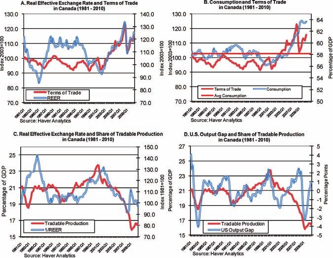
6           International Journal of Central Banking                 March 2012

disease.2 The Dutch disease phenomenon is a source of concern for
policymakers to the extent that a smaller tradable sector might
undermine future possibilities of growth and employment creation.
In this context, policymakers face a key question: What type of
policy intervention can counteract the negative effects of a Dutch
disease episode? In this paper we evaluate the merits of one of the
policy options commonly implemented by governments: exchange
rate stabilization through monetary policy.
    One way to prevent tradable output from falling below the effi-
cient level is to depreciate the real exchange rate through monetary
policy. A policy of exchange rate depreciation can be successful in
preventing a contraction of tradable output, but it will have alloca-
tive effects in the economy. In this paper we evaluate in a dynamic
stochastic general equilibrium (DSGE) model what the cost and
benefits of this policy intervention are in terms of macroeconomic
stability and welfare.
    To illustrate the effects of a Dutch disease episode, figure 1 shows
the behavior of several Canadian macroeconomic variables in recent
years. In the period 2002–07, the terms of trade improved 25 per-
cent. This increase in the terms of trade was driven by a worldwide
boom in commodity prices—in particular, a surge in oil and gas
prices. Consistent with the empirical evidence of commodity cur-
rencies, panel A shows that the real effective exchange rate also
appreciated around 25 percent.3 These changes in relative prices
had an impact in the reallocation of resources across sectors in the
economy. For instance, panel B shows that the ratio of consumption
to GDP increased about 8 percentage points in the same period,
reflecting the wealth effects from higher commodity prices.
    On the other hand, panel C shows the share of manufactur-
ing production over GDP for Canada. The period of exchange rate
appreciation coincides with a contraction of 4 percentage points of

    2
     The term “Dutch disease” was introduced to describe the situation experi-
enced in the Netherlands in the 1960s after the discovery of gas deposits in the
North Sea. The discovery of natural resources was followed by an appreciation of
the real exchange rate and a crowding out of the manufacturing exports. More
recently, the term is also used to describe the negative effects on exports induced
by foreign aid, remittances, capital inflows, or an improvement in the terms of
trade.
   3
     For a reference on commodity currencies, see Chen and Rogoff (2003).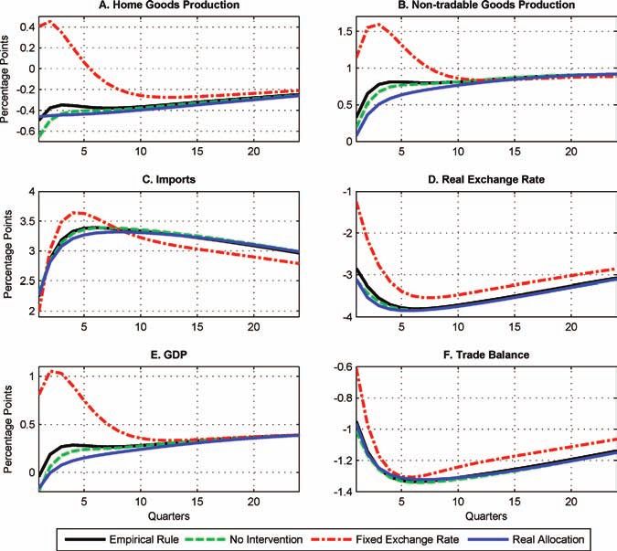
Vol. 8 No. 1              Exchange Rate Stabilization              7

  Figure 1. Effects of Higher Terms of Trade in Canada

GDP in the share of manufacturing production. Notice that this real-
location process is unprecedented in the Canadian economy in terms
of the size and the timing of the contraction. Panel D shows that in
the last twenty years, Canadian manufacturing production experi-
enced a maximum contraction of 2 percentage points of GDP every
time it entered into a recession, which coincides with a recession in
the United States. The most recent episode of exchange rate appreci-
ation shows a larger decline in manufacturing production unrelated
to the U.S. business cycle, pointing out some Dutch disease effects in
the economy. We consider Canada an interesting case study to the
extent that it is an economy with a sizable manufacturing export
sector and, at the same time, with business cycles sensitive to vari-
ations in commodity prices. These two features make the potential
costs of a Dutch disease episode larger compared with other small
open economies.
    In a standard frictionless two-sector real business-cycle model,
the reallocation between the tradable and non-tradable sector, such
8          International Journal of Central Banking               March 2012

as the one observed in Canada, is the efficient response to an
increase in the terms of trade. Higher terms of trade will increase
the demand for tradable and non-tradable goods, and as a conse-
quence wages will be higher in the economy. Taking international
prices as given, higher wages will reduce the production of tradable
goods, and the demand will be satisfied with imports from the rest
of the world. In this situation there is no rationale for government
intervention, and protecting the tradable sector will reduce overall
welfare.
    If we consider an economy with nominal rigidities in domestic
prices, then variations in the terms of trade can reduce welfare if
these variations generate domestic inflation volatility. In this situa-
tion, the role of monetary policy is to stabilize the set of prices with
nominal rigidities and allow the nominal exchange rate to adjust
freely. Considering Canada as an example, the policy prescription
to higher terms of trade in a model with nominal rigidities will be
to stabilize domestic inflation and allow a nominal exchange rate
appreciation in order to absorb the external shock. This policy leads
to a real exchange rate appreciation and hence to a reallocation of
resources from the tradable to the non-tradable sector, similar to
what has been observed in the Canadian case.
    However, if there are additional frictions besides nominal rigidi-
ties, the full flexibility of the exchange rate might not necessarily be
a desirable property of the optimal monetary policy, and some degree
of exchange stabilization might be required. In this work we focus on
one friction commonly discussed in the Dutch disease literature: the
learning-by-doing (LBD) externality in the tradable sector. Consid-
ering an LBD mechanism, a reduction in tradable output will lead
to lower productivity in that sector and a decrease of future produc-
tion. If this mechanism is not internalized by the firms, then there
will be an inefficient loss of tradable production and hence a role for
policy intervention.
    One policy option commonly used to influence tradable produc-
tion is stabilizing the exchange rate.4 Intervening in the foreign
exchange rate market can prevent a fall of tradable production below

    4
    For empirical evidence on exchange rate stabilization across countries, see
Calvo and Reinhart (2002).
Vol. 8 No. 1                    Exchange Rate Stabilization                        9

the efficient level. However, if we consider nominal rigidities in alter-
native sectors of the economy, as the empirical evidence suggests,
then an intervention in the foreign exchange rate market could also
induce a misallocation of resources.5,6 Policymakers face a trade-off
between correcting the LBD externality in the tradable sector and
ensuring an efficient allocation of resources across productive sectors.
In the paper we evaluate this trade-off and analyze how successful
a policy of exchange rate stabilization is in addressing the potential
inefficiencies during a Dutch disease episode.7
    The main result of the paper is that exchange rate intervention
is a welfare-reducing policy to counteract the effects of the Dutch
disease. On the one hand, a policy of exchange rate stabilization
can prevent a contraction of tradable production below the efficient
level. On the other hand, stabilizing the exchange rate exacerbates
the effects on aggregate demand generated by an improvement of
the terms of trade and hence increases macroeconomic volatility.
In a version of the model calibrated to the Canadian economy, we
find that the costs in terms of macroeconomic volatility and misal-
location of resources far exceed any benefits obtained from a more
stable exchange rate. The intuition for this result is that exchange
rate intervention through monetary policy is a blunt instrument
to correct the LBD externality. Stabilizing the exchange rate not
only expands tradable output but also stimulates all sectors in the
economy in tandem, which turns out to be highly distortionary in
a context of higher terms of trade. These conclusions are robust
to several modifications of the baseline model such as larger LBD

   5
     For a reference of sticky prices in alternative sectors of the economy, see Bils
and Klenow (2004).
   6
     If we assume that prices in some sectors of the economy are sticky and the
nominal exchange rate is stabilized, then the real exchange rate adjustment is
going to come partially from an increase in domestic inflation. If we assume
either a pricing behavior as in Rotemberg (1982) or Calvo (1983), the higher
inflation induced in the sticky sectors due to the exchange rate stabilization
will generate a loss of resources in those sectors and hence a misallocation of
resources.
   7
     In this paper we consider the case of exchange rate stabilization through the
short-term interest rate. Under the assumption of perfect asset substitutability
of domestic and foreign bonds, the stabilization through the short-term interest
rate and foreign exchange rate intervention are equivalent.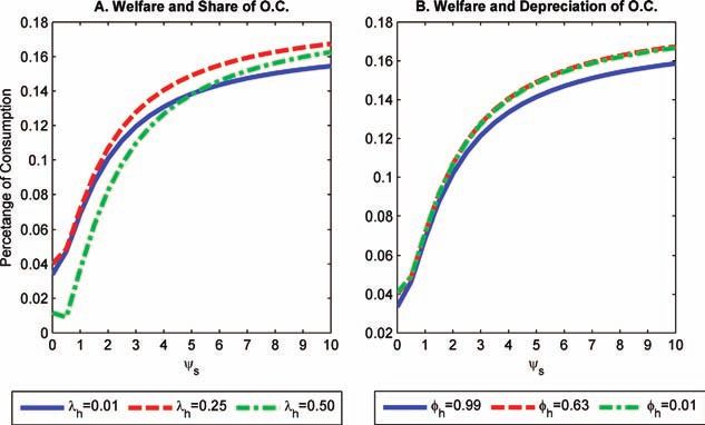
10         International Journal of Central Banking        March 2012

externalities, LBD in the non-tradable sector, incomplete exchange
rate pass-through for imported goods, and alternative preferences
that eliminate the wealth effects on labor supply.
    This paper is related to an extensive Dutch disease literature.
Van Wijnbergen (1984), Krugman (1987), and Caballero and Loren-
zoni (2009) evaluate alternative policy interventions in the context of
Dutch disease episodes. These authors differ regarding which friction
generates a misallocation of resources in response to an appreciated
exchange rate. The first two authors consider an LBD externality in
the tradable sector, while Caballero and Lorenzoni analyze the case
of financial frictions in the exportable sector. Our paper also con-
ducts a policy evaluation in response to a Dutch disease, considering
as the starting point a New Keynesian small open-economy model.
The framework is similar to the work of Adolfson et al. (2007), Lubik
and Schorfheide (2007), and Justiniano and Preston (2008), who esti-
mate and evaluate different versions of the New Keynesian model for
small open economies. We depart from these models by introducing
an LBD mechanism in the manufacturing exportable sector. Chang,
Gomes, and Schorfheide (2002) and Cooper and Johri (2002) pro-
vide empirical evidence regarding the quantitative importance of the
LBD mechanism. This paper contributes to the Dutch disease lit-
erature by performing a quantitative evaluation on the merits of
exchange rate stabilization to correct the LBD externality.
    A caveat is in order. Our model assumes transitory variations of
the terms of trade and temporary effects of the learning-by-doing
externality on tradable output. Hence, we resort to a first-order
approximation around a well-defined steady state to solve for the
model. In practice, however, some countries might experience highly
persistent shocks that can have permanent effects on the size of the
manufacturing sector. For those episodes, the use of global methods
could be a better approach to evaluate policy options for long-lasting
effects of the Dutch disease.
    The rest of the paper is organized as follows. Section 2 describes
the small open-economy model. Section 3 discusses the calibration
strategy for the model. Section 4 presents the main findings of the
paper. Section 5 shows the welfare analysis. Section 6 characterizes
the optimal fiscal and monetary rules in response to a Dutch dis-
ease episode. Section 7 presents some model extensions. Section 8
concludes.
Vol. 8 No. 1 Exchange Rate Stabilization 11
2. A Small Open Economy with Learning-by-Doing
In this section we present a multi-sector small open-economy model
with nominal rigidities and an LBD externality in the tradable sec-
tor. The model is built along the lines of Christiano, Eichenbaum,
and Evans (2005), Adolfson et al. (2007), and Smets and Wouters
(2007). We depart from these models by introducing LBD external-
ity in the tradable sector following Chang, Gomes, and Schorfheide
(2002) and Cooper and Johri (2002). The model captures two fea-
tures of economies that can be exposed to a Dutch disease: a large
commodity sector and an LBD externality in the manufacturing sec-
tor. This last feature generates a misallocation of resources during
a boom of commodity prices and calls for government intervention.
The model considers three sectors. The first sector produces a
manufactured home good (H).8 The second produces a non-tradable
good (N ). The third produces a commodity good, which is exported
entirely at a given international price. Consumer preferences are
defined over final consumption good and leisure. The model con-
siders sticky prices in the tradable and non-tradable sector which
generate real effects for changes in monetary policy. The key inno-
vation with respect to standard New Keynesian models is the intro-
duction of an LBD externality in the manufacturing tradable sector.
Appendix 1 describes all the equilibrium conditions of the model.
2.1 Households
The household’s preferences are defined over consumption and labor:
∞
Ut = Et β i u(Ct+i − hHt+i , Lt+i ) , (1)
i=0
where Lt is labor effort, Ct is its total consumption, and the exter-
nal habit component is defined by Ht+i = Ct+i−1 . Households have
access to three types of assets: money Mt , one-period non-contingent
foreign bonds Bt∗ , and one-period domestic contingent bonds Dt+1
8
For the rest of the paper, we are going to use the terms tradable production
and home goods production indistinctively, referring to the good that is produced
domestically and can be exported.12 International Journal of Central Banking March 2012
which pay out one unit of domestic currency in a particular state.9
The household budget constraint is given by
PtC Ct + Et {dt,t+1 Dt+1 } + Et Bt∗ + Mt =
∗
Wt Lt + Πt + Dt + Et Bt−1 1 + i∗t−1 Θ((Bt−1 )) + Mt−1 ,
where PtC is the price of consumption, Πt is profits received from
all domestic firms, Wt is the nominal wage, and Et is the nominal
exchange rate. dt,t+1 is the period t price of one-period domestic
contingent bonds divided by the probability of the occurrence of the
state. The financial costs of the foreign bond Bt∗ are defined by the
foreign interest rate i∗t and the risk premium Θ(.).10
2.2 Firms
There are four types of firms in the economy: final goods produc-
ers, retailers, intermediate goods producers, and capital producers.
Next, we describe the structure of all these firms.
2.2.1 Final Goods Producers
The final goods producers YtF combine home-produced inputs YtDH ,
imports YtM , and non-tradable inputs YtDN according to a constant
elasticity of substitution (CES) production function:
ηY
1/ηY T YηY DN ηYη −1 ηY −1
η −1
YtF = αY Yt + (1 − αY )1/ηY
Yt Y , (2)
ωY
1/ωY DH ω M ωωY −1 ωY −1
ωY −1
YtT = γY Yt Y + (1 − γY )1/ω Y
Yt Y , (3)
9
In the model, money plays the role of a unit of account. Considering an
alternative specification, such as separable money in the utility function, does
not modify the quantitative results of the model.
10
This premium is a function of the net foreign asset positions relative to GDP,
Et Bt∗
Bt = PY,t Yt
, where PY,t Yt is nominal GDP and Bt∗ is the aggregate net asset posi-
tion of the economy. This premium is introduced as a technical device to ensure
stationarity (see Schmitt-Grohé and Uribe 2003).Vol. 8 No. 1 Exchange Rate Stabilization 13
where YtT denotes the production of tradable inputs. αY and ηY
are the share of tradable inputs and the elasticity of substitution for
the final goods production function, respectively. γY and ωY are the
share of domestic inputs and the elasticity of substitution for the
tradable goods production function.
2.2.2 Retailers
We assume that firms in the retail sector sell home goods YtH
and non-tradable goods YtN in two separate stages. First, there
is an assembler that combines the differentiated intermediate good
indexed by j ∈ [0, 1] in each sector J = H, N to produce YtJ . The
technology is a constant elasticity of substitution aggregator given by
J
1 J −1 J −1
YtJ = YtJ (j) J
dj , (4)
0
where J is the elasticity of substitution between a variety of goods.
The optimal choice for each assembler yields a demand function for
intermediate goods:
−J
PtJ (j)
YtJ (j) = YtJ , (5)
PtJ
1
1 1−J
PtJ = PtJ (j)1−J dj . (6)
0
Second, retailers of each intermediate good have monopolistic
power and set their prices according to the Calvo (1983) framework.
Every period, a fraction (1 − θJ ) of retailers in sector J = H, N
set their prices optimally. The optimal price PtJ∗ (j) chosen by each
retailer maximizes the expected present value of profits:
∞
P J∗
t (j) − P WJ
t+i
Et (θJ )i Λt,t+i J
J
Yt+i (j) , (7)
i=0
P t+i
where Λt,t+i is the stochastic discount factor, and PtW J is the whole-
sale price of the intermediate good of sector J = H, N . PtW J is deter-
mined competitively in the intermediate goods market. The problem
of the intermediate goods producers is explained in the next section.14 International Journal of Central Banking March 2012
2.2.3 Intermediate Goods Producers
There is a continuum of firms in the non-tradable sector. Each firm
n ∈ [0, 1] produces output YtN (n) using physical capital and labor,
KtN (n) and Lt (n), respectively. The production function is given by
ηN 1−ηN
YtN (n) = AN N
t Kt (n) LN
t (n) , (8)
where AN,t denotes an aggregate productivity shock in the sector.
The tradable sector is subject to an LBD externality. The pro-
duction function of each representative firm h ∈ [0, 1] in this sector
is given by
ηH γH
YtH (h) = AH
t [Ht (h)]
λH
KtH (h) LH
t (h) , (9)
where AH H H
t , Kt (h), and Lt (h) denote an aggregate productivity
shock, capital, and labor, respectively. Ht (h) is the level of organi-
zational capital in the home goods sector. We restrict the technology
to the case of constant returns to scale, that is, λH + ηH + γH = 1.
The organizational capital evolves according to the following law of
motion:
H μH
Ht+1 (h) = [Ht (h)]φH Y t , (10)
H
where Y t is the production at the industry level, (1 − φH ) is the
depreciation rate of organizational capital, and μH is the elasticity
of organizational capital with respect to current output. We restrict
the exponents of the law of motion to the case of constant returns
to scale, that is, φH + μH = 1. This is the same specification as in
Cooper and Johri (2002). These authors found empirical evidence
for this specification of LBD using plant-level and national income
and product accounts data. In a more recent paper, Clarke (2008)
found evidence of LBD in the Canadian manufacturing sector.
In this paper, we follow the same interpretation of organiza-
tional capital as in Lev and Radhakrishnan (2003): “Organizational
capital is thus an agglomeration of technologies—business prac-
tices, processes and designs, including incentive and compensation
systems—that enable some firms to consistently extract out of a
given level of resources a higher level of product and a lower cost thanVol. 8 No. 1 Exchange Rate Stabilization 15
other firms.” Hence in the model, higher production in the tradable
sector leads to an increase in organizational capital, which improves
the efficiency in the sector and generates additional production with
the same level of labor and physical capital.
2.2.4 Capital Producers
Capital producers J = H, N own and rent sector-specific capital to
firms in the home and non-tradable goods sectors, respectively. The
aggregate investment of each type of capital is a composite of home,
foreign, and non-tradable goods as in the case of the final good. The
representative firm of each type of capital J solves the following
problem:
∞
J
Zt+i J
Kt+i − Pt+i
C J
It+i
J
Vt = max Et Λt,t+i C
,
J ,I J
Kt+i t+i i=0
Pt+i
subject to the law of motion of physical capital:
ItJ
J
Kt+1 = (1 − δ)KtJ + S J
ItJ , (11)
It−1
where ZtJ is the rental rate of physical capital, VtJ is the present
discounted value of profits, and δ is the depreciation rate of capital
in sector J. S(.) characterizes the adjustment cost for investment.11
2.3 Commodity Sector
We assume that the exports of commodities Xt in this economy
evolve exogenously according to the following process:
Xt = [Xt−1 ]ρx [X0 ]1−ρx exp εxt , (12)
11
We follow Christiano, Eichenbaum, and Evans (2005) and specify an invest-
ment adjustment cost that satisfies the following conditions: S(1) = 1, S (1) = 0,
S (1) = −μS < 0. This assumption generates inertia in investment that is
consistent with a time-to-build specification.16 International Journal of Central Banking March 2012
where εxt ∼ N (0, σx2 ) is a stochastic shock and ρx measures the per-
sistency of the process.12 We assume that the commodity price Ptx
follows the stochastic process
ρpx 1−ρpx
Ptx = Pt−1 x
P0x exp εpx
t , (13)
where εpx
t ∼ N (0, σpx ) is a stochastic shock and ρpx measures the
2
persistency of the commodity prices.
2.4 Monetary Policy Rule
The monetary policy is characterized by a Taylor-type rule:
(1−ψi )ψy
πC,t(1−ψi )ψπ st(1−ψi )ψs
ψi
1 + it 1 + it−1 Yt
= ,
1+i 1+i Yt π s
(14)
where it , Yt , πC,t , and st are the nominal interest rate, GDP, CPI
inflation, and the nominal exchange rate depreciation, respectively.
The parameters ψy , ψπ , and ψs are the weights assigned in the Tay-
lor rule to stabilize deviations of output, inflation, and depreciation
rate, with respect to their steady-state values. The parameter ψi
indicates the degree of interest rate smoothing in the Taylor-type
rule. In the rule, the key parameter that is going to be evaluated is
the intensity of exchange rate stabilization ψs .
2.5 Market Clearing Conditions
In every period, markets clear for labor, capital, intermediate home
and non-tradable goods, the final good, and international bonds.
The market clearing conditions for labor and capital are given by
1 1
Lt = LN
t (n)dn + LH
t (h)dh , (15)
0 0
1
KtJ = KtJ (j)dj , J = H, N. (16)
0
12
We assume an exogenous process for commodity exports to simplify the
model. In section 7 we consider a more realistic setup in which the commod-
ity sector hires physical capital and labor. In that case, the main qualitative
results of the model are not modified.Vol. 8 No. 1 Exchange Rate Stabilization 17
The market clearing conditions for home and non-tradable inter-
mediate goods are
YtDN = YtN , (17)
YtDH + CtH∗ = YtH , (18)
∗
where CtH∗ = γ ∗ ( Et PH,t −η
Ct∗ is the foreign demand for home goods,
P
∗ )
F,t
and Ct∗ is the aggregate foreign consumption. Finally, the equi-
librium conditions in the final goods production and international
bonds are given by
YtF = Ct + ItH + ItN , (19)
Et Bt∗ = 1 + i∗t−1 Θ(Bt−1 )Et Bt−1
∗
+ PtM YtM − PtH CtH∗ − Ptx Xt .
(20)
3. Calibration and Solution Method
To evaluate the quantitative predictions of the model, we log-
linearize the equations around the steady state. To ensure stationar-
ity of the model, we introduce a risk premium term that depends on
the net foreign asset position (see Schmitt-Grohé and Uribe 2003).
We use the algorithm proposed by Schmitt-Grohé and Uribe (2004b)
to solve the rational expectations model, which provides an efficient
implementation of the solution method proposed by Blanchard and
Kahn (1980).13
The model is calibrated to match some features of the Canadian
data, as an example of a small open economy exposed to terms-of-
trade shocks. Table 1 describes the parameter values used in the
calibration of the model. Most of the parameters for the real block
of the model are obtained from the Bank of Canada Quarterly Pro-
jection Model (Murchison and Rennison 2006) and are in line with
the literature of monetary policy in open economies.14 We calibrate
13
For the welfare analysis, we resort to a second-order approximation using the
algorithm developed by Schmitt-Grohé and Uribe (2004b).
14
For the elasticity of the investment adjustment cost, we chose the value
μS = 2.5 taken from Christiano, Eichenbaum, and Evans (2005).18 International Journal of Central Banking March 2012
Table 1. Baseline Parameter Values
Description Symbol Value
Discount Factor β 0.99
Habit Persistence h 0.65
Labor Supply Elasticity 1/ϕ 0.60
Share of Tradable Inputs—Final αY 0.50
Goods Sector
Elasticity of Substitution—Final ηY 0.50
Goods Sector
Share of Home Inputs—Tradable γY 0.50
Goods Sector
Elasticity of Substitution—Tradable ωY 0.50
Goods Sector
Depreciation Rate δ 0.02
Capital Share—Non-Tradable Sector ηN 0.30
Labor Share—Non-Tradable Sector 1 − ηN 0.70
Capital Share—Home Goods Sector ηH 0.20
Labor Share—Home Goods Sector γH 0.55
Learning Rate—Home Goods Sector λH 0.25
Calvo Parameter—Home Goods θH 0.75
Sector
Calvo Parameter—Non-Tradable θN 0.75
Sector
Elasticity of Substitution—Home εH 6
Goods Sector
Elasticity of Substitution— εN 6
Non-Tradable Sector
Foreign Interest Rate Elasticity (Θ /Θ)Bt 0.001
Foreign Demand Elasticity η∗ 0.50
Depreciation Rate—Organizational 1 − øH 0.37
Capital
Output Elasticity—Organizational μH 0.37
Capital
Interest Rate Smoothing ψi 0.70
Coefficient—Taylor Rule
Inflation Coefficient—Taylor Rule ψπ 1.30
Output Coefficient—Taylor Rule ψy 0.23
Depreciation Coefficient—Taylor ψs 0.14
RuleVol. 8 No. 1 Exchange Rate Stabilization 19
the model so each time period is one quarter. The utility function is
logarithmic in consumption with a constant labor supply elasticity:
L1+ϕ
u(Ct − hHt , Lt ) = log(Ct − hHt ) − ζL t
,
1+ϕ
where Lt is labor effort, Ct is its total consumption, and the exter-
nal habit component is defined by Ht = Ct−1 . Consistent with the
evidence of Taylor (1999) and Nakamura and Steinsson (2008), we
set the frequency of price adjustment to four quarters. In the base-
line calibration, we assume that nominal rigidities are present in the
home goods and non-tradable goods sectors.15
The Taylor-type rule parameters are obtained from Lubik and
Schorfheide (2007). These authors use Bayesian techniques to esti-
mate a specification of the Taylor rule for Canada in which the
nominal interest rate responds to variations of GDP, inflation,
and exchange rate depreciation, and has a smoothing component.
Finally, the LBD parameters are obtained from Cooper and Johri
(2002). The share of organizational capital in the production func-
tion is λH = 0.25, which corresponds to a learning rate of 20 percent
found in the literature. Consistent with the empirical evidence, the
depreciation rate of organizational capital is 1−φH = 0.37. Following
Schmitt-Grohé and Uribe (2001), we assume that the elasticity of the
risk premium with respect to debt is close to zero (Θ /Θ)Bt = 0.001,
which induces stationarity without affecting the quantitative prop-
erties of the model.
Using data for Canada for the period 1981:Q1–2008:Q4, we esti-
mate the following processes for the shocks affecting the economy:
t = 0.96at−1 + t , t ∼ N 0, σH , σH = 0.015,
aH T H H 2
(21)
t = 0.97at−1 + t , t ∼ N 0, σN , σN = 0.005,
aN N N N 2
(22)
t , t ∼ N 0, σX , σX = 0.017,
xt = 0.86xt−1 + X X 2
(23)
where aH N
t , at , and xt are the log-deviations of home goods sector
productivity, non-tradable sector productivity, and production in
15
In section 7 we also consider a model with incomplete exchange rate pass-
through, where importers have the ability to set prices in the domestic market.20 International Journal of Central Banking March 2012
the commodity sector (mining, gas, and oil).16 The commodity price
shock and the external demand shock are estimated using data on
oil prices and U.S. consumption:
pX X
t = 0.94pt−1 + t , t ∼ N 0, σP2 X , σP X = 0.15,
PX PX
(24)
c∗t = 0.99c∗t−1 + ∗t , ∗t ∼ N 0, σC
2
∗ , σC ∗ = 0.006, (25)
∗
where pXt and ct are the log-deviations of commodity prices and
foreign consumption.
4. Findings
4.1 Effects of Learning-by-Doing
This section reports the quantitative effects of LBD in the economy.
Figure 2 shows the impulse response function when the economy is
affected by a transitory increase of one standard deviation of com-
modity prices. The solid lines represent the dynamics of a standard
New Keynesian model without the LBD externality and the dashed
lines represent the dynamics of the model laid out in section 2 includ-
ing external LBD. Both models consider the same monetary policy
rule with the parameters laid out in table 1. To gain intuition about
how shocks are propagated in the model, first we explain the dynam-
ics of the small open economy without LBD and then the dynamics
with this externality.
The solid lines in figure 2 show the reallocation process experi-
enced in the economy in response to an increase of one standard devi-
ation of commodity prices. Consistent with a standard two-sector
model, the commodity shock induces a reallocation from the tradable
sector to the non-tradable sector. In response to higher commod-
ity prices, there is a higher demand for tradable and non-tradable
goods. Considering that international prices of tradable goods are
given, this higher demand for non-tradable goods will induce a real
exchange rate appreciation and a reallocation of resources from the
16
Even though our model allows for the possibility of stochastic shocks to the
endowment of the commodity sector, in the simulation results shown in table 2
we shut down that shock. The difference in the simulations with and without
endowment shocks is quantitatively small. The simulation of the model with the
endowment shocks is available upon request.Vol. 8 No. 1 Exchange Rate Stabilization 21
Figure 2. Effects of Learning-by-Doing
tradable to the non-tradable sector. At the same time, a higher
demand for tradable goods is satisfied with imports from the rest
of the world. As a result of the expansion of non-tradable produc-
tion, GDP will increase, and as a consequence of lower tradable
production and more imports, the trade balance deteriorates.17
The dashed lines in figure 2 describe the dynamics of the model
with LBD. Two effects are operating in the model with LBD. First,
in response to a decline in home goods production, the amount of
organizational capital decreases through the law of motion (10).
17
In the impulse response function, we show the trade balance excluding the
commodity exports to better assess the effects of higher commodity prices.22 International Journal of Central Banking March 2012
A lower organizational capital reduces the overall productivity of
the home goods sector, which exacerbates the initial contraction in
production, as shown in panel A. Second, lower productivity in the
home goods sector increases the price level in the small open econ-
omy, which leads to a higher value of the real exchange rate, as
shown in panel D. As we can appreciate in panels E and F, lower
production of home goods and a further real exchange rate appreci-
ation leads to smaller expansion of GDP and a further deterioration
of the trade balance.
Overall, the main effects of LBD in the model are a decline of
tradable production, GDP, and the trade balance. Clearly, this exter-
nality reduces welfare of households. In the next sections we evaluate
how successful a policy of exchange rate stabilization is in correcting
this externality.
4.2 Learning-by-Doing and Exchange Rate Stabilization
In this section we evaluate the impact of alternative policy rules to
correct the frictions associated with price rigidities and the LBD
externality. We consider three types of monetary policy rules which
differ in their degree of exchange rate intervention: the empirical
monetary policy rule, a monetary policy rule with no exchange rate
intervention, and a fixed exchange rate policy. For the first rule we
use the baseline calibration summarized in table 1. The empirical
estimates from Lubik and Schorfheide (2007) indicate a moderate
amount of exchange rate intervention, given the parameter value
ψs = 0.14. In addition to this baseline calibration, we consider two
polar cases: first, the case of no intervention, in which ψs = 0, and
second, the case of a fixed exchange rate regime, where ψs −→ ∞.
We compare the dynamics of these rules with the allocations
of a benchmark model with flexible prices and internalized LBD.18
When LBD is internalized, there is a price for organizational capital
that allows firms and households in the economy to decide the effi-
cient amount of employment, physical capital, organizational capital,
and production for the sector. The real allocation of the benchmark
model indicates the best outcome a policy intervention can achieve
18
See appendix 2 for the first-order conditions of the benchmark model with
flexible prices and internalized learning-by-doing.Vol. 8 No. 1 Exchange Rate Stabilization 23
at business-cycle frequencies.19 Any discrepancy or deviation from
the benchmark model indicates a misallocation of resources in the
economy. We gauge if a particular monetary policy rule is welfare
improving if it is able to close the discrepancies or gaps with the
benchmark frictionless model. In the limit, the optimal policy will
generate an allocation that exactly coincides with the one from the
benchmark model.20,21
Figure 3 shows the impulse response function for the real allo-
cations of the benchmark model and three rules: the empirical rule,
a monetary rule with no exchange rate intervention, and a fixed
exchange rate. For the benchmark model, we observe a reallocation
of resources from the home goods sector to the non-tradable sec-
tor. Notice that even though the LBD externality is internalized,
it is optimal to allow for a contraction of the home goods sector.
In the benchmark model, we also observe an appreciation of the
real exchange rate and an expansion of GDP. To evaluate the suc-
cess of alternative policy rules, we have to measure how far from this
benchmark are the allocations generated by the alternative monetary
policy rules.
First we analyze the behavior of the monetary rule with no
exchange rate intervention (ψs = 0). Under this rule, home goods
production goes below the efficient level of output. In terms of the
New Keynesian literature, under this rule there is a negative output
gap in the home goods production. In principle, it is possible to close
this gap by engineering a monetary expansion that depreciates the
exchange rate and stimulates tradable output. However, it is impor-
tant for policymakers to evaluate what are the implications of an
exchange rate depreciation in other sectors of the economy.
19
An additional friction we consider in the model is monopolistic competition,
which generates a misallocation of resources at the steady state. Goodfriend and
King (2001) showed that monetary policy is not effective to remove the markup
of monopolistic competition at the steady state. If we additionally consider a
subsidy on employment, then it is possible to achieve the first-best allocation
with the combination of fiscal and monetary policy.
20
See Correia, Nicolini, and Teles (2008).
21
If we evaluate a variable such as production, a deviation with respect to the
benchmark model is consistent with the definition of output gap in a standard
New Keynesian model.24 International Journal of Central Banking March 2012
Figure 3. Learning-by-Doing and Exchange
Rate Stabilization
Now we consider the empirical rule which considers some
exchange rate intervention, that is, ψs = 0.14. This parameter
reduces the appreciation of the real exchange rate in response to
the commodity price shock. The empirical rule allows the produc-
tion of home goods to be closer to the efficient level; however, the
rest of the sectors are going to expand more than in the benchmark
model. Figure 3 shows how non-tradable production and imports are
larger than the efficient level, while the real exchange rate is going
to be more depreciated. In addition, GDP increases more than the
efficient level.
The third rule is a fixed exchange rate, which sets ψs → ∞.
Given that we consider sticky prices in the model economy, this pol-
icy is extremely successful in limiting the magnitude of exchangeVol. 8 No. 1 Exchange Rate Stabilization 25
rate appreciation in the short run. Nevertheless, all the quantities
in the small open economy overshoot the allocations compared with
the benchmark model, which reflects higher distortions. In sum, this
policy generates higher macroeconomic volatility and welfare costs
compared with other rules.
There are two main results from this section. First, monetary
policy is a very potent instrument to increase tradable production
and to prevent an inefficient outcome in this sector. Second, lean-
ing against an appreciated exchange rate generates greater macro-
economic volatility, measured by the deviations from the efficient
allocation. The initial impulse of higher commodity prices triggers
an expansion of aggregate demand in a commodity-exporting econ-
omy like Canada. In this situation, a policy of exchange rate sta-
bilization generates a further expansion of aggregate demand and
greater volatility over the business cycle. To evaluate whether or
not this is an appropriate policy, we need to compare the benefits
of higher tradable production against the costs of larger macroeco-
nomic volatility. In the next section we conduct a welfare analysis of
alternative policy rules to compare properly the costs and benefits
of stabilizing the exchange rate during a Dutch disease episode.
5. Business Cycles and Welfare Calculations
This section quantifies the welfare costs of alternative monetary pol-
icy rules. The welfare costs are calculated as in Lucas (1987) and are
measured as a fraction of consumption that agents are willing to give
up to eliminate the excess volatility of a specific policy. The welfare
of the benchmark model with flexible prices and internalized LBD,
denoted by B, and the welfare of a monetary regime, denoted by R,
are given by
∞
UB = E β t u CtB − hCt−1
B
, 1 − LB
t , (26)
t=0
∞
UR = E β t u CtR − hCt−1
R
, 1 − LR
t . (27)
t=0
Typically (26) is going to be greater than (27) since the bench-
mark model does not incorporate frictions such as price stickiness26 International Journal of Central Banking March 2012
Table 2. Simulated Business Cycles and Welfare Costs
Std. Dev. ×/ Std.
Std. Dev. Dev. GDP Welfare
GDP NX/GDP C INV L RER λ
Canadian Data 1.51 0.89 0.57 2.73 0.71 2.46 —
(1981–2008)
Empirical Rule 1.49 0.93 0.78 2.65 0.76 2.81 0.04
No Intervention 1.58 1.32 0.77 2.70 0.79 2.97 0.04
Fixed Exchange Rate 2.52 1.22 0.79 2.49 0.98 1.50 0.19
and LBD externality. In order to evaluate how costly is a specific
policy, we solve for the welfare cost, denoted by λ, in the following
equation:
∞
E β t u (1 − λ) CtB − hCt−1
B
, 1 − LB
t
t=0
∞
=E β t u CtR − hCt−1
R
, 1 − LR
t . (28)
t=0
The welfare cost is computed as in Schmitt-Grohé and Uribe
(2005) from the second-order approximation of equation (28). If a
specific policy generates welfare costs, then λ > 0, while if it is suc-
cessful to correct nominal rigidities and the LBD externality, then
λ = 0. To have a meaningful estimation of the welfare costs, first we
ensure that the model is able to reproduce some of the moments in
the data. Table 2 describes the second moments from the data and
the model, as well as the welfare costs of monetary policy rules.
The first row in table 2 reports some moments observed in the
Canadian data. We observe that consumption and employment are
less volatile than GDP, while investment and the real exchange rate
are about twice as volatile as output. The fact that consumption
is less volatile than GDP is not specific to Canada but is a feature
common to industrialized countries.22 On the other hand, investment
22
See Neumeyer and Perri (2005) and Aguiar and Gopinath (2007).Vol. 8 No. 1 Exchange Rate Stabilization 27
tends to be more volatile than output in most small open economies,
both industrialized and emerging.23
The second row in table 2 shows the results from simulating the
model with the calibrated empirical rule subject to the five shocks
described in section 3. Overall, the model with the empirical rule
matches the main features of the data. In the model, consumption
tends to be more volatile than in the data, but it is still the case that
consumption is less volatile than GDP, as is observed in developed
small open economies. The last column in the second row shows the
welfare cost as a fraction of the steady consumption. The empirical
rule generates a welfare cost equivalent to 0.04 percent of lifetime
consumption.
The third row shows the second moments and welfare calcula-
tion of the Taylor-type rule with no exchange rate intervention. The
results of this policy are very close to the empirical rule; however,
this Taylor-type rule allows for greater real exchange rate volatility.
This volatility spills over the trade balance, which has a standard
deviation 50 percent larger than in the case of the empirical rule.
In this case we also obtain welfare costs that are similar to the ones
obtained from the empirical rule, indicating that the allocations are
not quantitatively different among these policies.
The fourth row shows the fixed exchange rate policy. This rule
increases the volatility of GDP by 60 percent and the volatility of
labor by 25 percent, and at the same time reduces real exchange rate
volatility by 50 percent.24 As we analyzed in the previous section,
stabilizing the nominal exchange rate in response to an increase in
commodity prices can be achieved by increasing money supply. This
policy provides a further stimulus to the economy, in addition to an
increase in commodity prices, increasing output volatility and reduc-
ing households’ welfare. The welfare cost of this policy is equivalent
to 0.19 percent of lifetime consumption. This number is about two
times the measure of costs of business cycles estimated by Lucas
(1987). This welfare loss is generated mainly by the increase in labor
supply volatility by 25 percent.
23
See Schmitt-Grohé (1998).
24
Notice that since investment responds sluggishly owing to the investment
adjustment costs, most of the GDP variation in the short run is generated by
fluctuations of labor and productivity.28 International Journal of Central Banking March 2012
Figure 4. Welfare Costs and Exchange Rate Stabilization
Figure 4 depicts the welfare costs as a function of the exchange
rate intervention parameter ψs . The horizontal axis shows the depre-
ciation rate coefficient in the Taylor rule, and the vertical axis shows
the welfare costs measured by λ. This welfare analysis allows us to
better understand the welfare costs of exchange rate stabilization
for a wider spectrum of monetary rules.
In panel A we consider three assumptions for the share of organi-
zational capital: the baseline calibration in which λH = 0.25, then a
case of a low share, λH = 0.01, and finally the case of a high share in
which λH = 0.50. For the baseline calibration and the case of a low
share, welfare costs are an increasing function of exchange rate inter-
vention. As a central bank intervenes in the foreign exchange rate
market, the allocation in the economy tends to move away from the
efficient equilibrium, which is costly in terms of welfare. In particu-
lar, a policy of exchange rate stabilization increases macroeconomic
volatility, which affects negatively households’ welfare. Only when
the amount of LBD externality is twice the magnitude of the empir-
ical estimations (λH = 0.50) are there some gains derived from
moderate exchange rate interventions.25 When the exchange rate
25
See Cooper and Johri (2002).Vol. 8 No. 1 Exchange Rate Stabilization 29
stabilization coefficient ψs is below 1, then the benefits from protect-
ing the tradable sector outweigh the costs of higher macroeconomic
volatility, generating a reduction in welfare costs. When the coef-
ficient is greater than 1, the opposite case holds, and the costs of
macroeconomic volatility exceed any potential gain of stabilizing the
tradable sector.
In panel B we evaluate alternative assumptions on the depreci-
ation rate: the baseline case of φH = 0.63, the case of low depreci-
ation rate φH = 0.99, and finally the case of high depreciation rate
φH = 0.01.26 For the three assumptions of depreciation rate, the
more aggressive is the monetary policy rule to stabilize the nomi-
nal exchange rate, the larger are the welfare costs. Even though the
depreciation rate affects the persistency of the externality over time,
it does not change the main conclusion of table 2: more exchange
rate intervention increases macroeconomic volatility and the welfare
costs of the representative household.
The main result in this section is that a policy of exchange rate
intervention typically results in welfare losses. In spite of being an
effective instrument to correct inefficiencies in the home goods sec-
tor, the policy is costly in terms of macroeconomic volatility. This
result suggests that correcting the LBD externality with monetary
policy is highly distortionary for empirically plausible estimates of
the LBD externality. On the other hand, allowing an exchange rate
appreciation during a Dutch disease episode ensures an efficient allo-
cation of resources across sectors. This result is consistent with the
view of Friedman (1953) in favor of flexible exchange rates. In pres-
ence of nominal rigidities, a flexible exchange rate is capable of
insulating the economy from external shocks by generating a faster
adjustment of relative prices.
6. Optimal Fiscal and Monetary Policy Rules
In the previous sections we evaluated the impact of increasing the
extent of exchange rate stabilization on the resource allocation in
a small open economy. The main conclusion from the quantita-
tive analysis is that protecting the tradable sector with monetary
26
Recall that in the model the depreciation rate is given by (1 − φH ).30 International Journal of Central Banking March 2012
policy results in reduction in welfare and an increase in macroeco-
nomic volatility. Then, the natural question is: what policies are
appropriate to cope with Dutch disease episodes? In this section we
evaluate fiscal and monetary policy rules that can improve the allo-
cation of resources during a commodity boom. The fiscal rule is a
state-contingent subsidy rule (τtH ) on the production of home goods
designed to correct the LBD externality:
τtH = Et [f (xt , xt+1 , yt , yt+1 )], (29)
where xt and yt are the vectors of predetermined and jump variables
in the model, respectively. In appendix 2 we show the derivation of
the optimal subsidy rule. For the monetary policy rule we use the
same specification as in (14) and choose the coefficients of the rule
that maximize the unconditional welfare of the representative house-
hold. The resulting coefficients of the optimized Taylor-type rule are
given by ψπ = 2.23, ψi = 0.56, ψy = −0.76, and ψs = −0.25.27
The coefficients on GDP and exchange rate depreciation in the
optimized rule have negative signs, which are not consistent with the
empirical estimates. Ireland (1996) provides an explanation regard-
ing the existence of a negative GDP coefficient on the optimized
rule. He shows that in models with nominal rigidities and produc-
tivity shocks, the optimal monetary policy is procyclical.28 In the
context of our model, the presence of productivity shocks driving the
business cycle leads to a negative relationship between output and
the short-term rate in the optimal rule. Schmitt-Grohé and Uribe
(2004a) also show that expressing the optimal monetary policy in
terms of a Taylor-type rule leads to a negative coefficient on output.
In order to gain more intuition about the optimal coefficient
on exchange rate intervention, it is convenient to analyze the log-
linearized version of the Taylor-type rule:
it = ψiit−1 + (1 − ψi )(ψy yt + ψπ π̂t + ψs st ), (30)
27
Schmitt-Grohé and Uribe (2007) show that an optimized rule of this form
generates dynamics that approximate the Ramsey policy.
28
Since an increase in productivity reduces prices, the optimal policy increases
the money supply in order to stabilize the price level, resulting in a procyclical
monetary policy.Vol. 8 No. 1 Exchange Rate Stabilization 31
where the variable x t denotes the logarithmic deviations of the vari-
able xt from its steady state x, that is, x t = log(xt ) − log(x). In
equation (30) it , yt , π̂t , and st denote the logarithmic deviations
of the gross nominal interest rate, GDP, CPI inflation, and nom-
inal exchange rate depreciation, respectively. In addition, the CPI
inflation in log-linear form is defined as
π̂t = αY (γY )π̂tH + (1 − γY ) st + (1 − αY )π̂tN . (31)
Adopting the parameter values from the baseline calibration, we
get the following expressions:
it = 0.56it−1 + (1 − 0.56)(−0.76
yt + 2.23t π̂t − 0.25
st ) (32)
π̂t = 0.5π̂tN + 0.25π̂tH + 0.25
st . (33)
Finally, combining (33) and (32), we get the expression for the
optimal monetary policy rule:
it = 0.56it−1 + (1 − 0.56) − 0.76
yt + 1.12t π̂tN + 0.56t π̂tH + 0.31
st .
(34)
In equation (34) we observe that in fact the optimized rule allows
some exchange rate stabilization. This policy rule implies a larger
exchange rate volatility compared with a monetary policy rule that
targets exclusively CPI inflation. Even though in the initial opti-
mized rule (32) a central bank might be seen as “leaning with the
wind,” in practice it is focusing on exchange rate stabilization, giv-
ing a weight of 0.31 to exchange rate depreciation in the alternative
rule (34).
In figure 5 we analyze the dynamics of the optimized monetary
policy rule and we compare it against two benchmarks: a frictionless
model with flexible prices and internalized LBD and the full-blown
model with a non-tradable inflation-targeting rule that sets the non-
tradable inflation to the steady-state level πtN = π N . Similar to the
exercise conducted in section 4, the frictionless model indicates the
best possible outcome that a policy intervention can achieve.
Figure 5 shows that the dynamics of the model under the opti-
mized rule tracks fairly well the allocations obtained from the real
allocation of the frictionless model. Two variables show significant32 International Journal of Central Banking March 2012
Figure 5. Optimal Fiscal and Monetary Policy Rules
departures from the frictionless model: the home goods production
and the optimal subsidy, shown in panels A and F. Home goods pro-
duction experiences a larger contraction under the optimized rule
compared with the frictionless economy. On the other hand, the
subsidy is much higher compared with the efficient case.
The key difference between the home goods production in the
model with the optimized rule and in the frictionless model is the
presence of nominal rigidities in that sector.29 This discrepancy indi-
cates that the optimized monetary policy rule is less focused on
29
The optimal subsidy shown in panel G is correcting the LBD externality, so
the discrepancy between the dynamics of the model with the optimized rule and
the frictionless model can be attributed to the presence of nominal rigidities.Vol. 8 No. 1 Exchange Rate Stabilization 33
correcting the problem of nominal rigidities in the tradable sector.
To better understand why the optimized rule is not stabilizing the
tradable sector, it is useful to compare its performance with the
non-tradable inflation-targeting rule.
The non-tradable inflation stabilizes the markup in the non-
tradable sector and ensures a flexible price allocation in that particu-
lar sector.30 In figure 6 we can notice that the non-tradable inflation
targeting tracks very closely the optimized rule. The reason for the
similarity is that the optimized rule focuses on stabilizing the largest
sector exposed to nominal rigidities. In the baseline calibration, the
lion’s share of production is concentrated in the non-tradable sector,
and the frequency of price adjustment is the same across sectors,
hence the optimized rule will give a higher weight to stabilizing
non-tradable inflation.31 For our particular calibration, the dynam-
ics of the optimized rule are not quantitatively different from the
non-tradable inflation-targeting rule.
Finally, in panel F we observe that the optimal subsidy is
larger both under the optimized rule and the non-tradable inflation-
targeting rule. This can be explained by the fact that there is an
additional contraction of tradable output under the optimized rule,
which exacerbates the LBD externality. In this case, since the opti-
mal fiscal rule is designed to remove the effects from LBD, there is
an increase in the subsidy to expand tradable production and correct
the externality. In equilibrium, it is still the case that tradable pro-
duction drops below the efficient level due to the presence of nominal
rigidities.
The results from this section complement the findings in the pre-
vious sections. In response to an increase in commodity prices, the
optimal fiscal and monetary policy rules allow a real exchange rate
appreciation and a reallocation between tradable and non-tradable
goods. Any policy that prevents this reallocation process will result
in a reduction of welfare.
30
For an evaluation of the non-tradable inflation-targeting rule, see Lama and
Medina (2011).
31
Benigno (2004) makes a similar argument. In a currency union, if two coun-
tries have the same frequency of price adjustment, the optimal monetary policy
for the union will stabilize a weighted average of regional inflation rates, where
the weights are determined by the size of each country.34 International Journal of Central Banking March 2012
Figure 6. Model Extensions
7. Model Extensions
Now we consider alternative specifications of the model to assess the
robustness of our results. There are several dimensions in which we
could add more layers of realism to the model. In this section we
explore four modifications to the small open-economy model: LBD
in the non-tradable sector, local currency pricing (LCP), GHH pref-
erences, and endogenous oil production. All of these frictions are
commonly discussed in the literature and potentially can improve
the fit of the model to the data. For each of these specifications we
show the volatility of GDP, the volatility of home goods produc-
tion, and the real exchange rate relative to GDP and the welfare
cost as a function of the parameter ψs , which measures the extent ofYou can also read