Key Players in Economic Development - Ashani Amarasinghe Roland Hodler Paul A. Raschky Yves Zenou May 2020 - Google Sites
←
→
Page content transcription
If your browser does not render page correctly, please read the page content below
Key Players in Economic Development∗
                         Ashani Amarasinghe†              Roland Hodler‡
                            Paul A. Raschky§              Yves Zenou¶
                                             May 2020

                                              Abstract
      This paper analyzes the role of networks in the spatial diffusion of local economic
      shocks in Africa. We show that road and ethnic connectivity are particularly important
      factors for diffusing economic spillovers over longer distances. We then determine the
      key players, i.e., which districts are key in propagating local economic shocks across
      Africa. Using these results, we conduct counterfactual policy exercises to evaluate
      the potential gains from policies that increase economic activity in specific districts or
      improve road connectivity between districts.
      Keywords: Networks, spatial spillovers, key player centrality, natural resources, trans-
      portation, Africa.
      JEL classification: O13, O55, R12.

  ∗
     We thank Markus Brückner, Matthew Leister, George Marbuah, Martin Ravallion and Mathias Thoenig
as well as conference and seminar participants at the Australasian Development Economics Workshop,
Australasian Public Choice Conference, CSAE Conference, Development Economics Network Switzerland,
Econometric Society European Meeting, German Development Economics Conference, IDEAs-CDES Sum-
mer School in Development Economics, Swiss Development Economics Workshop, Monash University and
University of Melbourne for their helpful comments. We also thank Shaun Astbury, Thu Phan, and Georgie
Stokol for excellent research assistance. Ashani Amarasinghe gratefully acknowledges support of the Aus-
tralian Government through its Research Training Program Scholarship. Roland Hodler and Paul Raschky
gratefully acknowledge financial support from the Australian Research Council (ARC Discovery Grant
DP150100061). This research was supported in part by the Monash eResearch Centre and eSolutions-
Research Support Services through the use of the Monash Campus HPC Cluster.
   †
     Department of Economics, Monash University; email: ashani.amarasinghe@monash.edu.
   ‡
     Department of Economics, University of St.Gallen; CEPR, CESifo, and OxCarre; email:
roland.hodler@unisg.ch.
   §
     Department of Economics, Monash University; email: paul.raschky@monash.edu.
   ¶
     Department of Economics, Monash University, CEPR, and IZA; email: yves.zenou@monash.edu.

                                                   1
1 Introduction
In recent decades, the majority of African countries have experienced an unprecedented
period of aggregate economic growth. However, the gains from this rise in aggregate income
have been unequally distributed between individuals and regions within those countries
(Beegle et al., 2016). The reason for this could be that in many African countries, economic
activity is concentrated in a few geographic areas, and the geography, poor transport infras-
tructure, and ethnic heterogeneity may limit the extent of spatial economic spillovers (e.g.,
Brock et al., 2001; Crespo Cuaresma, 2011).
The aim of this paper is to estimate the extent of spatial economic spillovers between
African districts, to highlight the roles of geographic, transport, and ethnic networks in
the context of regional economic development, and to determine which districts are key in
propagating local economic shocks across Africa.
We first develop a simple theoretical model that describes how one district’s prosperity
depends on its economic activity and its connectivity with other districts in a multi-district
network framework. The first-order conditions are used to estimate an econometric model
of spatial spillovers in which the economic activity of one district depends on the economic
activity of neighboring districts, which are defined in terms of geographic, ethnic and road
connectivity networks.
We constructed a balanced panel dataset of 5,944 African districts (ADM2, second sub-
national level) and yearly data from 1997–2013, in which our measure of local economic
activity was nighttime light intensity. The basic econometric framework is a spatial Durbin
model that allows for spatial autoregressive processes with the dependent and explanatory
variables. We interpret the estimated coefficient of the spatial lag of the dependent variable
in this model as the effect of a district’s connectivity on its own economic activity. Our
preferred specifications include time-varying controls as well as district and country-year
fixed effects to account for all time-invariant differences across districts and country-year
specific shocks that affect every district in a country and year, respectively.
The major empirical challenge is that the estimated parameter is likely to be biased
due to reverse causality and time-varying omitted variables. We address this problem by
2applying an instrumental variables (IV) strategy that builds on the work by Berman et al.
(2017). In particular, we rely on cross-sectional variation in the neighboring districts’ mining
opportunities and fluctuations in the world price of the minerals extracted in these districts
as the sources of exogenous temporal variation in the examined districts’ performance. Note,
however, that the primary goal is not to obtain estimates to evaluate the importance of the
spatial lags but to have a well-identified spatial econometric model to show how economic
shocks propagate through a network. We show that, individually, geographic, ethnic, and
road connectivity all increase local economic activity, however, they impact local economic
activity in different ways.
We then turn to measuring the network centrality of all the districts in Africa. Our
estimated coefficients on the spatial lag variable allow us to calculate Katz-Bonacich and
key-player network centralities. Based on the key-player centrality, we determine the “key”
districts in African countries, i.e., the districts that contribute most to economic activity
across Africa. These districts are typically characterized by high local economic activity as
well as good connectivity.
We think that our approach has important implications for policymakers in Africa as
well as international donors and development agencies. A planner who decides where to
locate a particular developmental project or where to build a new or better road may
need to consider many aspects, but one of them should be the potential of this project to
generate spatial economic spillovers. Therefore, we conduct counterfactual exercises to show
how the estimated coefficients and the underlying network structure can inform us about the
aggregate economic effects of policies that increase economic activity in particular districts or
improve road connectivity between districts. These counterfactual policy exercises illustrate
how our approach and its results could help policymakers to design more informed economic
policies.
Our paper contributes to three main strands of the literature. First, we contribute to
the empirical literature on the effects of networks in economics.1 This literature has so
far mostly focused on using micro data to test predictions from network theory (see e.g.,
Calvó-Armengol et al., 2009, and Fletcher et al., 2020, for education, Boucher, 2015, for
1
For overviews of the economics of networks, see Jackson (2008) and Jackson et al. (2017).
3friendship networks, and Fletcher and Ross, 2018, for health behaviors). There are also
some recent papers that study network effects from a macroeconomic perspective (see, in
particular, Acemoglu et al., 2012, 2015, Carvalho, 2015). These papers study production or
supply chain networks and document that the structure of the production network (input-
output matrix) is key in determining whether and how microeconomic shocks – affecting
only a particular firm or technology along the chain – propagate throughout the economy
and shape macroeconomic outcomes. In this paper, our unit of observation is at the district
level, which combines micro and macro analyses of both spatial and social networks.
Second, we contribute to the small literature on testing key players. There are very few
papers that empirically calculate key players in networks (exceptions include König et al.
(2017), Lindquist and Zenou (2014); Liu et al. (2020); for an overview, see Zenou (2016)),
but they do not determine them for a whole continent. Moreover, in these studies, the
key players are determined at the individual level, which creates network formation issues
that are difficult to deal with. In our paper, this is not the case because the links between
districts are pre-determined by their locations.
Third, we contribute to the literature that studies the importance of transport networks
and, more broadly, market access for subnational economic development in Africa. Studies in
this area often focus on the construction of new highways, e.g., in China or India (Banerjee et
al. (2012), Faber (2014), Alder (2015)). Our counterfactual policy exercise of improving road
connectivity between districts is related to Alder (2015), who has studied the consequences
of a counterfactual Indian highway network that mimics the design of the Chinese highway
network. Like us, Storeygard (2016), Bonfatti and Poelhekke (2017), and Jedwab and
Storeygard (2018) have focused on road networks in Africa. However, we differ from these
papers by focusing on the importance of roads in shaping the spatial diffusion of economic
shocks across Africa. Those spillover effects could be driven by increased market access
(e.g., Donaldson (2018), Donaldson and Hornbeck (2016)), which is of importance for the
road and geographic networks. However, economic spillovers also occur because of numerous
other channels, such as technology diffusion or transfer payments, and our aim is to estimate
the aggregate spillover effects of those various channels.
42 A simple model
2.1 The case of a single network
2.1.1 Spillover effects
Consider a network linking different districts. A network (graph) ω is the pair (N, E)
consisting of a set of nodes (here districts) N = {1, . . . , n} and a set of edges (links) E ⊂
N ×N between them. The neighborhood of a node i ∈ N is the set Ni = {j ∈ N : (i, j) ∈ E}.
The adjacency matrix Ω = (ωij ) keeps track of direct links so that ωij ∈ ]0, 1] if a link exists
between districts i and j, and ωij = 0 otherwise.2 We assume that the adjacency matrix Ω
P
is row-normalized so that the sum of each of its rows is equal to 1, i.e., j ωij = 1 for all
i.3 In the data, Ω = (ωij ) will capture connectivity based on geography, the road network
or ethnicity.
We assume that the level of economic activity li of a district i is given by:
J
X
li = ρ ωij lj + Xi + εi (1)
j=1
Indeed, we assume that the economic activity of district i is simply a function of the economic
activity of neighboring districts, of the observable characteristics Xi (such as its population)
and unobservable characteristics εi of this district. In this equation, ρ captures the spillover
effects of economic activities between neighboring districts.
Observe that the total level of activity li of district i is given by (1) because we would
like to describe activities at the district level and, more importantly, the transmission of
economic shocks between districts. Our theoretical framework, and the empirical analysis,
implicitly acknowledge that there are a plethora of possible transmission channels (e.g.,
prices, wages, trade, or migration). However, the main focus of this paper is analyzing the
effect of a district’s position on the diffusion of economic shocks within a network. For
that purpose, applying a simple, network theoretical model to a more aggregate setting is
sufficient.
2
In spatial econometrics, the adjacency matrix is called the “connectivity matrix.” Throughout the
paper, we will use these terms interchangeably.
3
All our theoretical results hold if the adjacency matrix is not row-normalized.
52.1.2 One possible microfoundation
There are different ways one can microfound equation (1). Let us propose a simple way of
doing so. Assume that the level of prosperity pi of a district i is given by:
J
X
pi = Xi li + ρli ωij lj + li εi (2)
j=1
where, as above, li is the economic activity in district i, Xi captures the characteristics of
district i and εi is the error term. In sum, the prosperity level of a district is determined
by the district’s observable and unobservable characteristics, the economic activity of the
district, and the spillover effects of the economic activity of neighboring districts.
Assume that the entity in charge of district i (this could be an institution or a local
government or a local politician) chooses the district’s own economic activity level li , taking
as given the choices of all the other districts. The payoff function of the entity in charge of
district i is then given by:
J
1 X 1
Ui = pi − li2 = Xi li + ρli ωij lj + li εi − li2 (3)
2 j=1
2
Indeed, the payoff function consists of the prosperity level of district i minus the cost of
maintaining this prosperity level, which is, quite naturally, increasing in economic activity.
Then, taking the first-order condition of (3) leads to (1), which can be written in matrix
form as follows:
l = (I − ρΩ)−1 (X + ε) =: CBO
X+ε (ρ, ω) (4)
where l is a column-vector of li s, I is the identity matrix, and X and ε are the vectors corre-
sponding to the Xi s and εi s, respectively. In (4), CBO BO
X+ε (ρ, ω), whose ith row is Ci,Xi +εi (ρ, ω),
is the weighted Katz-Bonacich centrality (due to Bonacich, 1987, and Katz, 1953), where
the weights are determined by the sum of Xi and εi for each district i. Denote by µ1 (Ω) the
spectral radius of Ω. Then, if ρµ1 (Ω) < 1, there exists a unique interior equilibrium given
by (1) or (4). Since the adjacency matrix Ω is assumed to be row-normalized, it holds that
µ1 (Ω) = 1. Thus, the condition for existence and uniqueness can be written as ρ < 1.
62.1.3 Interpreting the network model
Consider again (1). Then, ρ has an easy interpretation. In social networks, it is called the
social or network multiplier. Here, it is the strength of spillovers in terms of nighttime lights
between neighboring districts. To illustrate this, consider the case of a dyad (two districts,
i.e., N = 2). For simplicity, assume that the two districts are ex ante identical so that
X1 + ε1 = X2 + ε2 = X + ε. In that case, if there were no network (empty network) so that
the two districts were not linked, then (1) will be given by:
l1empty = l2empty = X + ε
Consider now a network where the two districts are linked to each other (i.e., ω12 = ω21 = 1).
Then, if ρ < 1, we obtain:
X +ε
l1dyad = l2dyad =
1−ρ
In other words, because of complementarities, in the dyad, the level of activity of each
district is much higher than when the districts are not connected. The factor 1/(1 − ρ) > 1
is the network multiplier.4
2.2 The case of multiple networks
In the real world, there is more than one type of spillovers between districts. For example,
in our main specifications below, we use different adjacency matrices Ω = (ωij ) that keep
track of the (inverse) spatial distance between districts, the road network and the proximity
in terms of ethnicity. In that case, (1) would be written as:
J
X J
X J
X
li = ρ1 ω1,ij lj + ρ2 ω2,ij lj + ρ3 ω3,ij lj + Xi + εi (5)
j=1 j=1 j=1
4
Observe that if we keep the ex ante heterogeneity, if ρ < 1, we obtain:
l1 1 X1 + ε1 + ρ (X2 + ε2 )
=
l2 (1 − ρ2 ) X2 + ε2 + ρ (X1 + ε1 )
7where ρ1 > 0, ρ2 > 0 and ρ3 > 0. We now have three adjacency matrices Ω1 = (ω1,ij ),
Ω2 = (ω2,ij ) and Ω3 = (ω3,ij ), which are all assumed to be row-normalized.
This equation states that the spillover effects in terms of economic activities between dis-
tricts are affected differently by the ways we measure the “proximity” between neighboring
districts.5
3 Estimating Spatial Spillover Effects for African Dis-
tricts
We would like to estimate (5), whose econometric equivalent is a standard Spatial Durbin
model. We constructed a balanced panel dataset in which the units of observation were the
administrative regions in Africa at the second subnational level (ADM2), which we labelled
districts.6 The final dataset consisted of yearly observations for 5,944 districts from 53
African countries over the period 1997–2013.7 The average (median) size of a district was
39km2 (6km2 ), and the average (median) population was around 150,000 (55,000). In the
Online Appendix A, we provide a detailed description of all variables. Here, we provide a
quick description of our main variables.
3.1 Data description
Our outcome variable was nighttime light intensity based on satellite data from the the
National Oceanic and Atmospheric Administration (NOAA). From the raw satellite data,
NOAA removes readings affected by cloud coverage, northern or southern lights, readings
that are likely to reflect fires, other ephemeral lights, and background noise. The objective
5
As above, we can provide a microfoundation of this equation by assuming that the prosperity level of
a district is given by:
J
X J
X J
X
pi = Xi li + ρ1 li ω1,ij lj + ρ2 li ω2,ij lj + ρ3 li ω3,ij lj + li εi
j=1 j=1 j=1
Then, if µ1 (ρ1 Ω1 + ρ2 Ω2 + ρ3 Ω3 ) < 1, there exists a unique interior equilibrium given by (5).
6
In a robustness test presented in Table D.4 in the Online Appendix, we used 0.5 × 0.5 degree grid cells
instead of ADM2 regions and show that all our results are qualitatively the same.
7
Table A.1 in the Online Appendix lists all the African countries in our sample and provides the number
of districts per country.
8is that the reported nighttime lights are primarily man-made. The NOAA provides annual
data for the time period from 1992 onward in output pixels that correspond to less than one
square kilometer. The data is presented on a scale from 0 to 63, with higher values implying
more intense nighttime lights. Work by Henderson et al. (2012) and Hodler and Raschky
(2014) has already shown that nighttime light is a good proxy for economic development at
the national and subnational level, respectively, which makes this suitable for the present
work’s purpose.
To construct our dependent variable, Lightit , we took the logarithm of the average night-
time light pixel value in district i and year t. To avoid losing observations with a reported
nighttime light intensity of zero, we followed Michalopoulos and Papaioannou (2013, 2014)
and Hodler and Raschky (2014) in adding 0.01 before taking the logarithm.
We construct three connectivity matrices to measure spatial spillovers:
Ethnic connectivity - To measure ethnic connectivity between districts, we first overlayed
the district (ADM2) boundaries with the boundaries of the ethnic homelands from Murdock
(1959). Each district was assigned the ethnicity of the ethnic homeland in which it is located.
For districts that fell into more than one ethnic homeland, we assigned the ethnicity of the
ethnic homeland that covered the largest part of the district. We then constructed our
ethnic connectivity matrix, ωi,j , where an element was 1 if the ethnicity in district i was the
same as the ethnicity in district j and 0 otherwise.
Geographic connectivity - We based the weighting matrix for geographic connectivity on
geographic distance. We constructed this weighting matrix as follows. First, we calculated
the centroid of each district. Second, we calculated the geodesic distance di,j connecting
the centroids of districts i and j. Third, following Acemoglu et al. (2015), we measured
the variability of the altitude ei,j along the geodesic connecting the centroids of districts i
and j and used elevation data from GTOPO30. Finally, we calculated the inverse of the
altitude-adjusted geodesic distance as d˜i,j = 1/di,j (1 + ei,j ). The main specification used a
cutoff of 70 km (for reasons made explicit below). In this case, we set the spatial weight as
ωi,j = 1/d˜i,j if the geodesic distance di,j was less than 70 km and ωi,j = 0 otherwise.
Road connectivity - To construct connectivity via the road network, we obtained data
from OpenStreetMap (OSM). We accessed the OSM data in early 2016 and extracted infor-
9mation about major roads (e.g., highways and motorways) for the African continent. We
intersected these roads with the district boundary polygons and generated a network graph
of the road network. The resulting road connectivity matrix assigns a value equal to the
inverse of the road distance in km between districts i and j if they are connected via a major
road and 0 if they are not connected. We, again, constructed different weighting matrices
by truncating at different distance cutoffs.
Our identification strategy made use of cross-sectional information concerning the loca-
tion of mining projects and temporal variations in the world prices of the corresponding
minerals. Information on mining activity came from the SNL Minings & Metals database.
We used the point locations to assign the mining projects to districts and to identify all
districts where a mine was active for at least one year during our sample period. Across
Africa, 4% of all districts are mining districts. The indicator variable M ineri is equal to one
if district i had a mining project that extracted resource r and was active for at least one
year during our sample period. Data on the world prices of minerals was sourced from the
World Bank, IMF, USGS, and SNL.8 P ricert is the logarithm of the yearly nominal average
price of resource r in USD.
3.2 Empirical strategy
The aim of the empirical analysis is to estimate (5), whose econometric equivalent is:9
3 X
X J 3 X
X J X
M
Lightit = ρk ωk,i,j Lightjt + Xit β + ρm m
k ωk,i,j Xjt + αi + CTct + it , (6)
k=1 j=1 k=1 j=1 m=1
where ω1,i,j is the (i, j) cell of the adjacency matrix based on geographic connectivity; ω2,i,j
is the (i, j) cell of the adjacency matrix based on road connectivity; ω3,i,j is the (i, j) cell
of the adjacency matrix based on ethnic connectivity; Xit = Xit1 , ..., XitM , the (1 × M )
T
vector of time-variant, district-level characteristics, and β = β 1 , ..., β M , a (M × 1) vector
of parameters; ρm
k are the coefficients of the spatial lags; αi and CTct are district and
country-year fixed effects, respectively; and it is an error term that is assumed to be it ∼
8
See Table A.4 in the Online Appendix for more information on the data sources.
9
In the theoretical model, we do not have a spatial autoregressive process in the explanatory variables
as in (6), but it would be straightforward to include them as it only affects the exogenous variable Xi .
10N (0, σ 2 In ).10 We row-normalized the adjacency matrices, i.e., we normalized them so that
the sum of each row became equal to 1.
In this specification, local spillovers to other districts not only operate through the spatial
lag of the dependent variable but also occur due to spatial autoregressive processes in the
explanatory variables as well (Spatial Durbin Model). In the spatial context, spillovers
might not only run from district j to i but also from i to j. In addition, economic activity
(and, therefore, Lightjt ) might be simultaneously determined by other unobserved shocks.
Thus, estimating equation (6) using OLS can yield biased and inconsistent estimates.
To address this problem, we estimated a 2SLS model that exploits exogenous variation
in the economic value of mineral resources in the mining districts.11 The idea was that
more valuable mining districts increase spillover effects such that the level of economic
activity in neighboring districts will be positively affected. In particular, in the first stage,
we used interaction terms between the time-invariant indicators of mining activity and the
time-variant exogenous world prices for minerals as instrumental variables:
X J X
3 X M
Lightjt = γM Pjt + Xjt β + ρm m
k ωk,j,i Xit + αj + CTct + ujt , (7)
k=1 i=1 m=1
where
Rj
1 X
M Pjt ≡ (M inerj × P ricert ), (8)
Rj r=1
M inerj being the number of different minerals extracted in district j. Hence,
P
with Rj = r
for each mining region, this instrumental variable captures the average of the world prices
(in logs) for all minerals that are extracted in the relevant district at some time during the
sample period. For all other districts, this instrumental variable is zero.
Our identification strategy is based on the work by Berman et al. (2017), who focus on
the effect of exogenous variation in the economic value of mines on the likelihood of local
conflict. The use of the time-invariant indicator M inerj addresses the potential endogeneity
between economic activity and mining activity. Hence, our identification strategy operates
10
Table C.2 in the Online Appendix presents estimation results without control variables and with year
rather than country-year fixed effects.
11
The results are very similar if we estimate our model using a quasi-maximum likelihood approach as
suggested by Anselin (1988).
11as a differences-in-differences estimator, which exploits between-variation in a district’s suit-
ability for extracting specific minerals, combined with the exogenous time variation in the
world price of these minerals.
In order for this instrument to be relevant, it is key that fluctuations in world mineral
prices have a first-order effect on the mining districts’ economies. We know from Brückner et
al. (2012) that oil price shocks lead to an increase in per capita GDP growth at the country-
level (also see Brunnschweiler and Bulte (2008)) while works by Aragon and Rud (2013) and
Caselli and Michaels (2013) have shown that resource extraction can have positive effects
on local economic development. In our sample, 4% of all districts are mining districts. Min-
erals, however, account for a large proportion of export earnings in many African countries,
especially strategically important minerals such as diamonds, gold, uranium, and bauxite.
Given the small number of mining districts and the importance of minerals at the country
level, it seems plausible to assume that fluctuations in world mineral prices are relevant for
mining districts.
With respect to the instrument’s validity, our identification strategy rests upon the
assumption that price shocks in the mining sector in district j affect Lightit in district i
only through Lightjt . We took a number of measures to mitigate the risk of the exclusion
restriction being violated. First, we included district-fixed effects in equation (7), which
absorb all time-invariant characteristics at the district level, including suitability for mining
activity. The vector of country-year fixed effects accounts for any time-variant factors that
might simultaneously drive mineral prices and aggregated economic development. Second,
the work by Berman et al. (2017) showed that mining activity could lead to increased
conflict as parties dispute over ownership of lucrative mines. This, in turn, could adversely
affect economic activity. Therefore, we controlled for district-level conflict events in our
specifications. Third, the exclusion restriction also relies on the assumption of exogeneity
of world prices, i.e., no single district can affect the world price of a commodity. For this
reason, we conducted a robustness check of our specifications by excluding countries in the
top ten list of producers for any mineral.
The statistical inference in our setting is further complicated by the clustering structure
of the error terms in our econometric model. The traditional spatial clustering approach
12proposed by Conley (1999) imposes the same spatial kernel (geographic distance) to all units
in the sample. However, our empirical model does not only assume dependence based on
geographic distance but also relatedness through ethnic and road networks. Therefore, we
applied a novel estimator developed by Colella et al. (2018) that allowed us to account for
dependence across our observations’ error terms in a more flexible form.12 In practice, we
corrected for clustering at the network level where observations were assumed to belong to
the same cluster once they are linked through at least one of the three networks (geography,
ethnicity, roads).13
Our setting implies that we needed to estimate the local average treatment effect (LATE)
of economic shocks related to windfalls in natural resource rents. These shocks and the
resulting spatial spillovers may have very particular effects on consumption, investment,
and government expenditure. Moreover, we estimated the LATE for districts with a certain
network proximity to mining districts. In our sample, 31% of all districts were within
a geodesic or road distance of less than 70 km to a mining district or shared an ethnic
connection with a mining district. These districts might systematically differ from the
average African district. For these reasons, one needs to be careful when drawing more
general policy conclusions based on the estimated spatial spillover effects.
In addition, it is a priori unclear whether mining-related income shocks only generate
positive spillover effects for other districts. Windfalls in natural resource rents in one dis-
trict could lead to migration of labor and capital from other connected districts into the
mining district. A mining boom could also lead the government to shift public expenditure
and infrastructure projects away from nearby districts into the mining district. As such,
the estimated parameters of the spatial lags represent the net effect from mining-related
economic shocks in connected districts.
12
This procedure was implemented in Stata 14 using the “acreg” command by Colella et al. (2018).
13
Table D.3 in the Online Appendix presents the results using the standard Conley-type spatial clustering
approach (Conley 1999). Our results remain the same.
133.3 Estimation results
Table 1 presents our estimates from equations (6) and (7).14 We start with specifications
that include each weighting matrix individually. Column (1) provides the results of the OLS
estimates for ethnic connectivity while column (2) provides the comparable IV estimates.
The OLS estimates show that coefficient ρ1 (coefficient on Ethnicity W Lightjt ) was positive
and statistically significant. In column (2), we present comparable IV estimates. The
coefficient of interest in the first stage of the IV estimate, γ, was positive and statistically
significant. This, along with the high F statistics of the first stage, indicates that our
instrumental variable was a strong predictor of economic activity in district j. The coefficient
of interest of the second stage, ρ1 , was positive but not statistically significant.
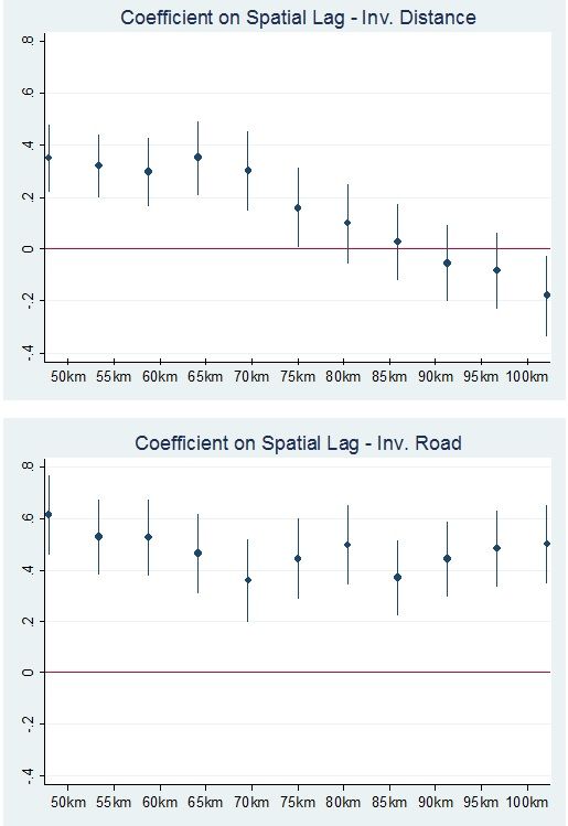
Second, we consider the inverse-distance connectivity. In Figure C.1 in the Online Ap-
pendix, we show that the coefficient of interest from the IV estimates declined in magnitude
in the cutoff distance and became statistically insignificant for cutoff distances beyond 70
km. As a result, in all our estimations, we truncated the adjacency matrix at 70 km. In
columns (3) and (4) of Table 1, we focus on geographic connectivity and, therefore, use the
weighting matrix based on the inverse of the altitude-adjusted geodesic distance between
districts i and j, truncating the matrix at 70 km. The coefficient of interest, ρ2 , was positive
and statistically significant at the 1% level in both the OLS and the IV estimations.
Third, in columns (5) and (6), we focus on road connectivity based on our matrix of
inverse road distances, again, truncating the matrix at 70 km. The coefficient of interest,
ρ3 , was positive and statistically significant at the 1% level in both the OLS and the IV
estimations. As in Figure C.1 in the Online Appendix, the coefficient of interest from the IV
estimates would remain positive and statistically significant for cutoff distances of 100 km
and beyond, indicating that the extent of positive spillovers spreads farther when focusing
on the actual transport infrastructure rather than just geography.
14
Table 1 only reports the coefficients on the variables of main interest to improve the readability of the
table. Table C.1 in the Online Appendix reports the coefficients on the control variables.
14Table 1: Connectivity based on ethnicity, geography and roads
(1) (2) (3) (4) (5) (6) (7) (8)
OLS IV OLS IV OLS IV OLS IV
Dependent variable: Lightit
Ethnicity W Lightjt 0.552*** 0.271 0.160*** 0.342***
(0.015) (0.176) (0.013) (0.122)
Inv Dist W Lightjt 0.550*** 0.639*** 0.246*** 0.305**
(0.012) (0.131) (0.011) (0.124)
Inv Road W Lightjt 0.556*** 0.280** 0.393*** 0.361***
(0.010) (0.113) (0.015) (0.116)
First stage: Dependent variable: Lightjt
M Pjt 0.121*** 0.124*** 0.119*** 0.123***
(0.015) (0.013) (0.014) (0.015)
15
First-stage F-stat 67.83 85.00 71.90 63.64
Observations 101,048 101,048 101,048 101,048 101,048 101,048 101,048 101,048
District FE YES YES YES YES YES YES YES YES
Country-year FE YES YES YES YES YES YES YES YES
Additional controls YES YES YES YES YES YES YES YES
Notes: The even columns report standard fixed effects regressions with district and country-year fixed effects, and
the odd columns report IV estimates. Ethnicity W Lightjt is weighted Lightjt , with weights based on the row-
normalized ethnicity matrix. Inv Dist W Lightjt (Inv Road W Lightjt ) is weighted Lightjt , with weights based on
the row-normalized matrix of the inverse altitude-adjusted geodesic distances (inverse road distances) truncated
at 70 km. Additional control variables include population, conflict, and M Pit as well as weighted population and
conflict in districts j 6= i. M Pjt is an interaction term based on cross-sectional information concerning the location
of mines and time-varying world prices of the commodities produced in these mines (see equation (8)). The first
stage further includes the control variables indicated in equation (7). Standard errors, clustered at the network
level, are in parentheses. ***, **, and * indicate significance at the 1, 5, and 10% levels, respectively.Finally, the last two columns of Table 1 include spatial lags with weights based on ethnic,
geographic, and road connectivity. That is, they report our estimates of the whole model
as described in equations (6) and (7). We observed that three coefficients of interest, i.e.,
ρ1 , ρ2 , and ρ3 , were all positive and statistically significant at the 1% level in the OLS
estimates. The same holds true for the IV estimates, except that the spatial spillovers
via purely geographic connectivity were only statistically significant at the 10% level. The
coefficient estimates further suggest that geographic connectivity tends to be less important
than ethnic and road connectivity.15
4 Most central districts
We now turn to the main aim of our paper: determining the districts that play a key role
in African economies due to their connectivity and their propagation of positive spillovers.
In fact, we can use our theoretical model, our connectivity matrices and our estimates of
the spillover effects to calculate various centrality measures and determine the districts that
play a key role in African economies due to their connectivity.
4.1 Theory: Different definitions of node centralities
There are different centrality measures (see Jackson, 2008, for an overview). We first intro-
duce two non micro-founded, purely topological centrality measures and then two micro-
founded measures that are strongly linked to our simple model.
4.1.1 Non micro-founded centrality measures
The two most commonly used individual-level measures of network centrality are between-
ness centrality and eigenvector centrality.
The betweenness centrality, CiBE (ω), describes how well located an individual district
in the network in terms of the number of shortest paths between other districts that run
through it. Denote the number of shortest paths between districts j and k that district i
15
In the Online Appendix D (Tables D.1–D.11), we conduct a series of robustness checks and show that
the estimates of the main coefficients remain similar.
16lies on as Pi (jk), and let P (jk) denote the total number of shortest paths between districts
j and k. The ratio Pi (jk)/P (jk) tells us how important district i is for connecting districts
j and k to each other. Averaging across all possible jk pairs gives us the betweenness
centrality measure of district i:
X Pi (jk)/P (jk)
CiBE (ω) =
(n − 1) (n − 2) /2
j6=k:i6∈{j,k}
It has values in [0, 1].
The eigenvector centrality, CiE (ω), is defined using the following recursive formula:
n
1 X
CiE (ω) = gij CjE (ω) (9)
µ1 (Ω) j=1
where µ1 (Ω) is the largest eigenvalue of Ω. According to the Perron-Frobenius theorem,
using the largest eigenvalue guarantees that CiE (ω) is always positive. In matrix form, we
have:
µ1 (Ω) CE (ω) = ΩCE (ω) (10)
The eigenvector centrality of a district assigns relative scores to all districts in the network
based on the concept that connections to high-scoring districts contribute more to the score
of the district in question than equal connections to low-scoring agents.
4.1.2 Katz-Bonacich centrality
In our theoretical model (Section 2), we have shown that the unique Nash equilibrium of our
game in terms of nighttime lights is equal to the Katz-Bonacich centrality of the district.
As a result, the level of nighttime lights in district i is given by its weighted Katz-Bonacich
centrality, defined in (4), i.e.
−1
CBO
X+ε (ρ, ω) =: (I − ρΩ) (X + ε)
Importantly, in order to calculate the Katz-Bonacich centrality of each district i, we
need to know the value of ρ. We will use the estimated value of ρ (IV estimates). We also
17need to check that the condition ρµ1 (Ω) < 1 is satisfied.
4.1.3 Key-player centrality
The Katz-Bonacich centrality was based on the outcome of a Nash equilibrium. Let us
now focus on the planner’s problem. The key question is as follows: Which district, once
removed, will reduce total nighttime lights the most? In other words, which district is the key
player? Ballester et al. (2006) have proposed a measure, key-player centrality, that answers
this question.16 For that, consider the game with strategic complements developed in the
n
theory section (Section 2) for which the utility is given by (3), and denote L∗ (ω) = li∗
P
i=1
the total equilibrium level of activity in network ω, where, assuming φµ1 (ω) < 1, li∗ is the
Nash equilibrium effort given by (1) or (4). Also, denote by ω [−i] the network ω without
district i. Then, in order to determine the key player, the planner will solve the following
problem:
max{L∗ (ω) − L∗ (ω [−i] ) | i = 1, ..., n} (11)
Then, the intercentrality or the key-player centrality CiKP (ρ, ω) of district i is defined as
follows:
BO
P
KP
Ci,u i
(ρ, ω) j mji (ρ, ω)
Ci,u (ρ, ω) = (12)
i
mii (ρ, ω)
BO
where Ci,u i
(ρ, ω) is the weighted Katz-Bonacich centrality of district i (see equation (4))
and mij (ρ, ω) is the (i, j) cell of the matrix M(ρ, ω)= (I − ρΩ)−1 . Ballester et al. (2006,
2010) have shown that the district i∗ that solves (11) is the key player if and only if i∗
is the district with the highest intercentrality in ω, that is, CiKP KP
∗ ,u (ρ, ω) ≥ Ci,u (ρ, ω), for
i i
all i = 1, ..., n. The intercentrality measure (12) of district i is the sum of i’s centrality
measures in ω, and its contribution to the centrality measure of every other district j 6= i
also in ω. It accounts both for one’s exposure to the rest of the group and for one’s
contribution to every other exposure. This means that the key player i∗ in network ω is
16
For an overview of the way the key player is determined in different areas, see Zenou (2016).
18given by i∗ = arg maxi Ci,u
KP
i
(ρ, ω), where17
∗ ∗
CiKP [−i]
∗ ,u (ρ, ω) = L (ω) − L ω . (13)
i
4.2 Empirical results
We computed these four different centrality measures for all 5,444 districts from the 53
African countries in our sample. In our discussion here, we will mainly focus on two large
countries that feature prominently in the literature: Nigeria and Kenya.18 Figure 1 compares
the key-player centrality of the districts (top row) with the districts’ average nighttime light
intensity (middle row) and population density (bottom row).
Column (4) of Table 2 presents the main ranking of interest, i.e., the key-player rank-
ing based on the geographic network, the road network and the ethnicity network. The
underlying computation thus uses the coefficient estimates, in particular the estimated ρ’s,
reported in column (8) of Table 1. The top 7 districts with the highest key-player centrality
are part of the Lagos metropolitan area which is the primate city of Nigeria and its eco-
nomic hub. Seven other districts belonging to the top-ten key districts of Nigeria are also
part of Lagos State. The two remaining districts in the key-player ranking belong to the
Kano metropolitan area which is the second largest metropolitan area in Nigeria and the
economic hub of the country’s north.
The key district in Kenya is Nairobi, which is the capital and the primate city. It is
followed by Mombassa, which is Kenya’s second largest city and home to Kenya’s largest
seaport (see the right column of Figure 1). The key districts encompass or are part of the
primate city in many other African countries as well, including Ethiopia (Addis Ababa)
and South Africa (Johannesburg). The overall pattern suggests that primate cities tend to
be the key districts development in Africa which resonates with the findings of Ades and
Glaeser (1995), Henderson (2002), or Storeygard (2016), among others.
Column (5) in Table 2 shows the ranking for the Katz-Bonacich centrality, again based
17
Ballester et al. (2006) define the key player in (12) only when the adjacency matrix Ω is not row-
normalized. Since we use row-normalized adjacency matrices when estimating the ρs, we will determine the
key player numerically based on its definition in (13).
18
Table E.1 in the Online Appendix presents the same information for the five most populous African
countries aside from Nigeria and Kenya.
19on the estimates taking the geographic network, the road network and the ethnicity network
into account. We see that the districts that rank high in terms of key-player centrality also
tend to rank high in terms of Katz-Bonacich centrality in Nigeria, but not in Kenya. This
is because Katz-Bonacich and key-player centralities capture different aspects of centrality.
The former is a recursive measure highlighting the importance of being connected to central
districts while the latter is a welfare measure that also takes into account the negative
impact of cutting links on neighboring districts.
Columns (6) and (7) show the rankings for the two other centrality measures: between-
ness and eigenvector centrality. Looking at Nigeria, we see that the districts from Lagos
State that are top ranked in terms of key-player centrality tend to rank poorly in terms
of these alternative centrality measures. This is not surprising given that the betweenness
and eigenvector centralities are pure topological measures, which capture either the number
of paths that go through a district (betweenness centrality) or the links to other central
districts (eigenvector centrality), and Lagos State is situated at the coast in the country’s
south-east bordering Benin.
Columns (8)-(10) also give rankings of key-player centrality, but in each of these columns
we compute the ranking based on the coefficient estimates from regressions including one
network only. We see that most districts that rank high in overall key-player centrality also
rank high in any type of single-network key-player centrality. This suggests that most key
districts are important due to their geographic, ethnic and road connectivity. For many
countries, the overall key-player centrality is most highly correlated with the key-player
centrality based on the road network, which indicates that road connectivity may be of
particular importance.
20Table 2: Top-Ten Key Player Rankings
(1) (2) (3) (4) (5) (6) (7) (8) (9) (10)
Country Province District Overall Overall Overall Overall Ethnicity Road Inv.Dist
KP Katz-Bon Betw. Eig. KP KP KP
Rank Rank Rank Rank Rank Rank Rank Rank
Nigeria
Nigeria Lagos Ikeja 1 16 564 428 4 1 2
Nigeria Lagos LagosIsland 2 24 707 424 32 2 18
Nigeria Kano Fagge 3 237 479 475 6 5 6
Nigeria Lagos Agege 4 14 641 433 8 14 4
Nigeria Lagos Ajeromi/Ifelodun 5 17 578 438 5 13 9
Nigeria Lagos Apapa 6 21 713 439 10 17 14
Nigeria Kano Tarauni 7 239 579 475 14 9 11
Nigeria Lagos Mainland 8 23 712 433 1 3 1
Nigeria Lagos Surulere 9 19 569 433 3 4 7
Nigeria Lagos Amuwo Odofin 10 12 432 440 26 7 12
21
Kenya
Kenya Nairobi Nairobi* 1 23 41 4 1 1 1
Kenya Coast Mombasa 2 41 45 8 2 2 2
Kenya Coast Kwale 3 37 9 8 17 48 3
Kenya Rift Valley Nakuru 4 20 3 26 8 4 5
Kenya Central Kiambu 5 24 40 5 4 3 4
Kenya Eastern Machakos 6 30 17 5 9 46 6
Kenya Central Murang’a 7 22 29 3 5 6 7
Kenya Central Nyeri 8 25 18 25 7 7 8
Kenya Rift Valley Narok 9 19 12 30 23 42 35
Kenya Central Kirinyaga 10 21 31 7 19 9 11
Notes: Overall KP Rank is based on the ρs estimated in column (8) of Table 1. Overall Katz-Bonacich Rank is based
on the ρs estimated in column (8) of Table 1 and a weighting vector of 1. Ethnicity KP Rank is based on ρ1 estimated
in column (2) of Table 1. Inv.Dist KP Rank is based on ρ2 estimated in column (4) of Table 1. Road KP Rank is
based on ρ3 estimated in column (6) Table 1. ∗ indicate districts that are (part of) capital cities. Nigeria has 775
districts, and Kenya has 48 districts.5 Policy experiments
The key-player rankings are valuable in showing which districts are most economically im-
portant. However, relying on key-player rankings for policymaking has two disadvantages.
First, the key districts are typically economically active and well-connected while policy-
makers may be interested in the benefits from either promoting local economic activity or
improving the network structure, e.g., by building roads. Second, key-player rankings cap-
ture the total effect of having a particular district while policymakers are generally better
advised to focus on the “marginal” effects of increasing local economic activity or improving
the network structure. In this section, therefore we illustrate how our approach allows for
counterfactual exercises that can inform policymakers.
5.1 Increasing local economic activity
The first policy experiment consists of increasing economic activity, i.e., nighttime lights,
in each district, one at a time. This experiment may mimic large public investments within
the given districts. We proceeded as follows. First, we added the value of 10 to the average
nighttime light pixel value in the treatment district, which corresponded to an increase of one
standard deviation.19 Second, we took the logarithm of the now higher average nighttime
light pixel value and recalculated the spatially lagged dependent variables with the new
values, while keeping the estimated ρ’s from Table 1 (column (8)). Third, we recalculated
the predicted nighttime lights (in logs) for each African district and computed the sum
across all districts. Fourth, we compared this sum, which included the increase in nighttime
lights in one district and the subsequent spatial spillovers, to the sum of the district-level
nighttime lights (in logs) across Africa from the baseline, i.e., in the absence of any policy
intervention. We repeated this exercise for each of the 5,944 districts.20
19
The nighttime light pixel values were top-coded at 63, and 0.01% of the districts in our sample had
average nighttime light pixel values above 53. Nevertheless, we increased the average nighttime light pixel
value of these districts by 10 as well.
20
In all steps and for all districts, we averaged the variables used over the sample period.
22Figure 1: Key-player Centrality, Nighttime Light Intensity, and Population Density in Nige-
ria and Kenya
Key-player centrality across Nigeria Key-player centrality across Kenya
Average nighttime lights across Nigeria Average nighttime lights across Kenya
Population density across Nigeria Population density across Kenya
Notes: Darker colors indicate higher values.
The maps in Panel (a) of Figure 2 show the districts in Nigeria (left panel) and Kenya
(right panel), where this counterfactual increase in economic activity would create a stronger
23(darker colors) and lesser (lighter colors) overall impact.21
There were various types of districts where the overall impact was particularly high.
First, for both Nigeria and Kenya, the districts with the highest impact also had high
key-player centrality because they are economically active and well-connected, such as the
districts from Lagos State. Second, in Nigeria, the top districts includes some districts in
Bayelsa and Delta, which are both oil-producing states in the Niger Delta. These districts
are economically quite active and well-connected, but they have a low key-player centrality
because they are conflict-ridden. An increase in economic activity, however, has a positive
impact exactly because of the dense network in the Niger Delta. Third, in Kenya, the
districts with the biggest impact included three poor districts that ranked at the bottom in
terms of key-player centrality because of their low nighttime light values. In these districts,
an increase in absolute nighttime lights leads to a large overall impact, mainly because we
measure economic benefits using the logarithm of nighttime lights. Our use of logged values
implies that an increase in economic activity is more valuable in poorer districts.
5.2 Improving road connectivity
The second policy experiment consisted of increasing the road connectivity of each district,
again one at a time. This experiment mimics improvements in the road infrastructure.
We proceeded as follows. First, for any given district, we determined the set of contiguous
districts with which the given district was not yet linked via a major road, and we chose
the district with the highest average nighttime light value from this set of districts. Second,
we added a link between these two districts (with a value of 1) in the non-normalized
road connectivity matrix. Third, we re-normalized the road connectivity matrix and then
recalculated the spatially lagged dependent and independent variables using this new matrix.
Fourth, we recalculated the predicted nighttime lights (in logs) for each African district and
computed the sum across all African districts. Finally, we, again, compared this sum with
the sum of nighttime lights (in logs) across Africa from the baseline. We repeated this
exercise for each of the 5,944 districts to identify the districts for each country that have
21
Table F.1 in the Online Appendix lists the Top 10 districts with the largest overall impact from this
counterfactual increase while Table G.1 presents the same ranking for the five other most populous African
countries.
24the largest overall impact when improving their road connectivity.
Panel (b) in Figure 2 maps the results of this policy experiment for districts in Nigeria
(left panel) and Kenya (right panel). Again, districts where a counterfactual improvement
of road connectivity would create a stronger overall increase in nighttime light are presented
by darker colors.22
The top districts in Nigeria are all in the Niger Delta. The top two, Boony and Orika, are
both islands with intense nighttime lights but poor road connectivity. Improving their road
connectivity would lead to positive economic spillovers from these two districts into other
districts in the Niger Delta and beyond. The districts with the strongest overall impact in
Kenya included many districts with high key-player centrality. In addition, the list included
some very dark/poor districts (Machakos, Wajir, and Meru), where an increase in economic
activity from better road connectivity would be particularly valuable. Along similar lines,
better road connectivity would also be of value in many dark/poor districts in Northeastern
Nigeria.
6 Concluding remarks
In this paper, we studied the role of geographical, ethnic, and road networks for the spatial
diffusion of local economic shocks using a panel dataset of 5,944 districts from 53 African
countries over the period 1997–2013. Our main aim was to calculate the key-player cen-
tralities by performing counterfactual exercises, which consisted of removing a district and
all its direct “links” (in the adjacency matrices representing the geographical, ethnic, and
road networks) and computing the economic loss to an average African district. We found
that primate cities are key for a country’s economic development due to their high economic
activity and good connectivity, suggesting that policies focusing on the major cities are jus-
tified from a growth perspective. We further conducted two counterfactual policy exercises;
the first increased economic activity in each district, one at a time, and the second each
district’s road connectivity.
22
Table F.2 in the Online Appendix lists the top 10 districts with the largest overall impact from this
counterfactual increase while Table G.2 presents the same ranking for the five other most populous African
countries.
25Figure 2: Results of the Counterfactual Policy Experiments - Nigeria and Kenya
Panel (a): The Counterfactual Increase in Economic Activity
Nigeria Kenya
Panel (b): The Counterfactual Improvement in Road Connectivity
Nigeria Kenya
Notes: Darker colors indicate a higher overall impact.
These counterfactual exercises illustrate the potential of our approach for informing
policymakers in Africa as well as international donors and development agencies. A planner
who decides where to locate a particular developmental project or where to build a new or
better road may need to consider many aspects, but one of them should be the potential of
this project to generate spatial economic spillovers. Therefore, we conducted counterfactual
exercises to show how the estimated coefficients and the underlying network structure can
inform us about the aggregate economic effects of policies that increase economic activity
in particular districts or improve road connectivity between districts.
26References
Acemoglu, D., Carvalho, V.M., Ozdaglar, A. and A. Tahbaz-Salehi (2012), “The network
origins of aggregate fluctuations,” Econometrica 80, 1977–2016.
Acemoglu, D., Garcia-Gimeno, C. and J.A. Robinson (2015), “State capacity and economic
development: a network approach,” American Economic Review 105, 2364–2409.
Ades, A. and E. Glaeser (1995), “Trade and circuses: Explaining urban giants,” Quarterly
Journal of Economics 90, 195–228.
Alder, S. (2015), “Chinese roads in India: the effect of transport infrastructure on economic
development,” unpublished manuscript, University of North Carolina at Chapel Hill.
Anselin, L. (1988), Spatial Econometrics: Methods and Models, Dordrecht: Kluwer Academic
Publishers.
Aragon, F.M. and J.P. Rud (2013), “Natural resources and local communities: evidence
from a Peruvian gold mine,” American Economic Journal: Economic Policy 5, 1–25.
Ballester, C., Calvó-Armengol, A. and Y. Zenou (2006), “Who’s who in networks. Wanted:
the key player,” Econometrica 74, 1403–1417.
Ballester, C., Calvó-Armengol, A. and Y. Zenou (2010), “Delinquent networks,” Journal of
the European Economic Association 8, 34–61.
Banerjee, A., Duflo, E. and N. Qian (2012), “Transportation infrastructure and economic
growth in China,” NBER Working Paper 17897.
Beegle, K., Christiaensen, L., Dabalen, A. and I. Gaddis (2016), Poverty in a Rising Africa,
Washington, DC: World Bank Publications.
Berman, N., Couttenier, M., Rohner, D. and M. Thoenig (2017), “This mine is mine! How
minerals fuel conflicts in Africa,” American Economic Review 107, 1564–1610.
Bonfatti, R., and S. Poelhekke (2017), “From mine to coast: transport infrastructure and
the direction of trade in developing countries,” Journal of Development Economics 127,
91–108.
Boucher, V. (2015), “Structural homophily,” International Economic Review 56, 235–264.
Brock, W.A. and S.N. Durlauf (2001), “What have we learned from a decade of empirical
research on growth? Growth empirics and reality,” World Bank Economic Review 15,
27You can also read