Kinetic mass-transfer calculation of water isotope fractionation due to cloud microphysics in a regional meteorological model - Atmos. Chem. Phys
←
→
Page content transcription
If your browser does not render page correctly, please read the page content below
Atmos. Chem. Phys., 19, 1753–1766, 2019
https://doi.org/10.5194/acp-19-1753-2019
© Author(s) 2019. This work is distributed under
the Creative Commons Attribution 4.0 License.

Kinetic mass-transfer calculation of water isotope fractionation
due to cloud microphysics in a regional meteorological model
I-Chun Tsai1 , Wan-Yu Chen2,3 , Jen-Ping Chen2,4 , and Mao-Chang Liang5
1 Research   Center for Environmental Changes, Academia Sinica, Taipei, Taiwan
2 Department    of Atmospheric Sciences, National Taiwan University, Taipei, Taiwan
3 Central Weather Bureau, Taipei, Taiwan
4 International Degree Program on Climate Change and Sustainable Development,

National Taiwan University, Taipei, Taiwan
5 Institute of Earth Sciences, Academia Sinica, Taipei, Taiwan

Correspondence: Jen-Ping Chen (jpchen@ntu.edu.tw)

Received: 15 June 2018 – Discussion started: 19 July 2018
Revised: 27 November 2018 – Accepted: 14 December 2018 – Published: 8 February 2019

Abstract. In conventional atmospheric models, isotope ex-           1   Introduction
change between liquid, gas, and solid phases is usually as-
sumed to be in equilibrium, and the highly kinetic phase            The water stable isotopes (1 H2 O, 1 H2 D16 O, and 1 H18
                                                                                                                          2 O) dif-
transformation processes inferred in clouds are yet to be           fer in molecular symmetry and weight. These differences
fully investigated. In this study, a two-moment microphysi-         in physical properties lead to a change in the stable iso-
cal scheme in the National Center for Atmospheric Research          tope composition of water, due to fractionation during phase
(NCAR) Weather Research and Forecasting (WRF) model                 changes. When water vapor condenses and forms liquid or
was modified to allow kinetic calculation of isotope fraction-      solid particles, it becomes depleted in 2 D and 18 O, because
ation due to various cloud microphysical phase-change pro-          heavy isotopes condense preferentially to light ones. Infor-
cesses. A case of a moving cold front is selected for quantify-     mation about the stable water stable isotopes is thus useful
ing the effect of different factors controlling isotopic compo-     for understanding the water cycle (Dansgaard, 1964; Dawson
sition, including water vapor sources, atmospheric transport,       and Ehleringer, 1998; Lorius et al., 1985; Risi et al., 2012;
phase transition pathways of water in clouds, and kinetic-          Sturm et al., 2010).
versus-equilibrium mass transfer. A base-run simulation was            Isotope fractionation, as measured in precipitation, has
able to reproduce the ∼ 50 ‰ decrease in δD that was ob-            been studied for decades. The observed isotope concentra-
served during the frontal passage. Sensitivity tests suggest        tions generally exhibit significant variations in either time
that all the above factors contributed significantly to the vari-   or space. Factors such as the effects of surface type (e.g.,
ations in isotope composition. The thermal equilibrium as-          land versus ocean), latitude, temperature, and precipitation
sumption commonly used in earlier studies may cause an              amount are commonly considered to be key to the relation-
overestimate of mean vapor-phase δD by 11 ‰, and the max-           ship between isotope fractionation and meteorological pa-
imum difference can be more than 20 ‰. Using initial verti-         rameters (Dansgaard, 1964; Gonfiantini, 1985; Rozanski et
cal distribution and lower boundary conditions of water sta-        al., 1993; Yurtsever and Gat, 1981; Kurita, 2013; Zwart et
ble isotopes from satellite data is critical to obtain successful   al., 2018). These factors are related to various physical pro-
isotope simulations, without which the δD in water vapor can        cesses, such as the surface water vapor source, atmospheric
be off by about 34 ‰ and 28 ‰, respectively. Without micro-         transport, phase changes in clouds, and gravitational sorting
physical fractionation, the δD in water vapor can be off by         of precipitation hydrometeors. For example, the water sta-
about 25 ‰.                                                         ble isotopic ratios decreased inland from the coast and the
                                                                    so-called continental effect (Clark and Fritz, 1997). The pre-
                                                                    cipitation amount effect states that isotopic contents of trop-

Published by Copernicus Publications on behalf of the European Geosciences Union.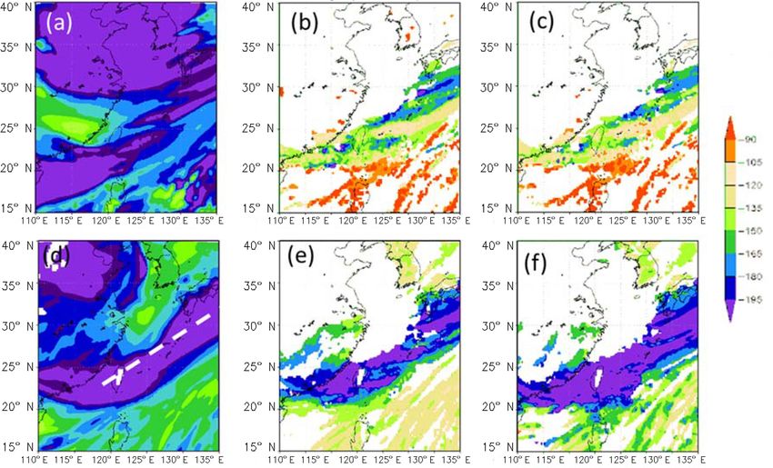
1754                                                                        I-C. Tsai et al.: Kinetic mass-transfer calculation

ical precipitation decrease as the amount of local precip-        to understand the role of different factors in the fractionation
itation increases (Dansgaard, 1964; Kurita, 2013), and the        of the stable isotopes of water at the synoptic scale.
cause of which could either be the preferential removal dur-         Because the αl-v of 18 O (grey line in Fig. 2) does not de-
ing condensation (Cole et al., 1999; Yoshimura et al., 2003)      viate significantly from unity, the signal of 18 O fractiona-
or stronger downdraft in more intense convection (Risi et         tion is generally much less pronounced. Therefore, we fo-
al., 2008). Untangling the intertwined effects of the various     cus on deuterium for demonstrating the fractionation pro-
physical processes is essential to understanding isotope frac-    cesses. The microphysical processes of deuterium such as
tionation and the atmospheric water cycle.                        condensation and collision were incorporated into the WRF
   The variations in isotope concentrations usually have mul-     model. A moving frontal system is selected to demonstrate
tiple causes, and it is difficult to understand the impacts of    the effect of microphysical fractionation versus other con-
different factors by measurements alone. Therefore, numer-        trolling factors such as air mass origins and surface sources.
ical models have been used to simulate isotope fractiona-         The effects of microphysical processes, including kinetic-
tion in the atmosphere. The Rayleigh-type models, in which        versus-equilibrium treatments, are discussed in more detail,
the air mass is continuously cooled down and the condensa-        whereas the importance of initial and boundary conditions of
tion process is assumed to occur in isotopic equilibrium, are     the vapor-phase isotope is also investigated.
widely used in discussing isotope measurements (Aldaz and
Deutsch, 1967; Dansgaard, 1964). Such models can explain
the linear relationship between the surface temperature and       2     Methodology
isotopic composition of precipitation (Rozanski et al., 1993),
and they have been expanded to incorporate more processes         In this study, the WRF model version 3.4.1 coupled with a
since the publication of Dansgaard (1964). For example,           two-moment bulk-water microphysical scheme (cf. Cheng et
Jouzel and Merlivat (1984) reported that the isotopic equilib-    al., 2010, 2015; Dearden et al., 2016) that was developed at
rium assumption led to an overestimation of the temperature-      the National Taiwan University (hereafter, the NTU scheme)
isotope gradients of polar snow, so they included isotopic ki-    was selected for simulations. The NTU scheme shown in
netic effects at snow formation in the models. However, the       Fig. 1 is modified to handle the isotope fractionation due
Rayleigh-type models greatly simplify the complexity of the       to various cloud microphysical phase-change processes. The
hydrological cycle, and Joussaume et al. (1984) introduced        hydrodeoxygenation (HDO) cycle and its initial and bound-
the concept of building isotopes into an atmospheric gen-         ary conditions were incorporated into the model and more
eral circulation model (AGCM). AGCMs can calculate the            details were provided in Sect. 2.1. The simulation setup and
transport and mixing of air masses from different sources         observation data are given in Sect. 2.2 and 2.3, respectively.
(which cannot be addressed by the Rayleigh-type models),
                                                                  2.1    Description of the isotopic microphysical model
and have been used in studying the hydrological cycle in the
troposphere (Hoffmann et al., 1998; Lee et al., 2007; Sjolte
                                                                  In modified NTU scheme, isotope mass transfer between
and Hoffmann, 2014; Yoshimura et al., 2008). In conven-
                                                                  vapor-, liquid-, and ice-phase hydrometeors during micro-
tional AGCMs, isotope exchange between liquid or ice and
                                                                  physical processes such as deposition, sublimation, evapora-
gas phases is usually assumed to be in a partial or full equi-
                                                                  tion, and condensation were considered explicitly (cf. Fig. 1).
librium state (Hoffmann et al., 1998; Risi et al., 2010; Nus-
                                                                  For processes of collision collection or melting and freezing,
baumer et al., 2017; Werner et al., 2011; Yoshimura et al.,
                                                                  the masses of isotopes of the involving particles are simply
2010). In a synoptic weather system such as a front or ty-
                                                                  combined or conserved, respectively, without worrying about
phoon, thermal equilibrium fractionation may not be appro-
                                                                  the fractionation.
priate for describing fractionation during phase change, since
                                                                     Thermal equilibrium fractionation has been widely used
the clouds are usually not in vapor equilibrium (Laskar et
                                                                  in conventional models. In such schemes, the HDO concen-
al., 2014). Therefore, in recent years, several regional mod-
                                                                  tration can be determined from the H16   2 O (hereafter, H2 O)
els start to consider the kinetic fractionation during evapora-
                                                                  concentration for both gas and liquid phases, because it is
tion from open water, condensation from vapor to ice, or iso-
                                                                  assumed that HDO is always in equilibrium with H2 O, irre-
tope exchange from raindrops to unsaturated air (Hoffmann
                                                                  spective of their phase states. The equilibrium between sta-
et al., 1998; Yoshimura et al., 2010; Blossey et al. 2010;
                                                                  ble isotopes in liquid water and vapor phases is commonly
Pfahl et al., 2012; Dütsch et al., 2016). However, the mi-
                                                                  expressed using the isotopic fractionation factor αl-v :
crophysics in these global or regional models is usually de-
scribed with single-moment schemes. This study developed a                 Rl
kinetic fractionation scheme for water stable isotopes using      αl-v ≡      ,                                                (1)
                                                                           Rv
a two-moment microphysical scheme that coupled into the
National Center for Atmospheric Research (NCAR) Weather           where R is the ratio of the heavy (HDO) to light (H2 O)
Research and Forecasting (WRF) model (Skamarock, 2008)            isotopes. This ratio can be explained with the Raoult’s law,
                                                                  which states that the activity (saturation ratio) of each species

Atmos. Chem. Phys., 19, 1753–1766, 2019                                             www.atmos-chem-phys.net/19/1753/2019/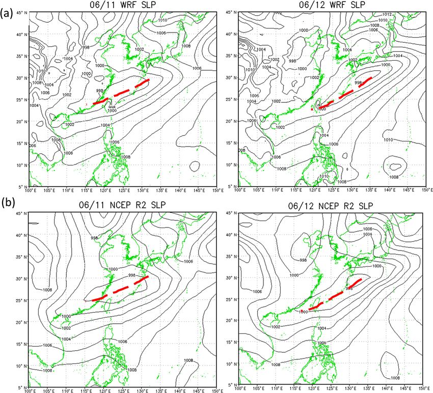
I-C. Tsai et al.: Kinetic mass-transfer calculation                                                                                 1755

Figure 1. Schematics of the modified NTU scheme. The blue boxes are the six hydrometeor categories considered in the model, and H/D
indicates that both H2 O and HDO are included. The arrows represent the microphysical conversion processes, and the light blue boxes
represent aerosol categories, including cloud condensation nuclei (CCN), giant CCN (GCCN), and ice nuclei (IN). Here Accr. denotes
accretion, and Evap denotes evaporation. (Figure modified from Cheng et al., 2010.)

                                                                              nHDO          PHDO
                                                                                          =         ,                                (2a)
                                                                          nHDO + nH2 O+nx   Ps,HDO
                                                                               nH2 O        PH2 O
                                                                                          =         ,                                (2b)
                                                                          nHDO + nH2 O+nx   Ps,H2 O
                                                                          where n is the number of moles in the liquid phase, P is
                                                                          vapor pressure, and Ps is saturation vapor pressure, whereas
                                                                          x represents all other chemical species. By dividing Eq. (2a)
                                                                          by (2b), one can derive the following:
                                                                          nHDO
                                                                          nH2 O       Ps,H2 O
                                                                          PHDO
                                                                                  =           .                                       (3)
                                                                                      Ps,HDO
                                                                          PH2 O

                                                                          One can see that the left-hand-side term is exactly αl-v , while
Figure 2. The ratio between saturation pressure of H2 O and HDO in
different phases (liquid: red line, solid: blue line) at different tem-
                                                                          the right-hand-side term tells us that this factor is actually
peratures. The grey line is the ratio of 18 O based on Horita and         the ratio between the saturation vapor pressure of H2 O and
Wesolowski (1994). The dashed lines are the formulas from Merli-          HDO. Thus the isotopic fractionation factor αl-v is a function
vat and Nief (1967).                                                      of temperature only and can be determined experimentally.
                                                                          In this study, we adopted the temperature dependence of αl-v
                                                                          from Horita and Wesolowski (1994):
in the vapor phase equals its activity in the liquid phase. For                                   3             2
the HDO–H2 O system, this relationship can be expressed as                   3                     T                T
                                                                          10 × ln αl-v = 1158         9
                                                                                                        − 1620.1                      (4a)
the following:                                                                                     10              106
                                                                                                                           !
                                                                                                                       109

                                                                                            T
                                                                               + 794.84       3
                                                                                                  − 161.04 + 2.9992          ,
                                                                                           10                          T3

www.atmos-chem-phys.net/19/1753/2019/                                                         Atmos. Chem. Phys., 19, 1753–1766, 2019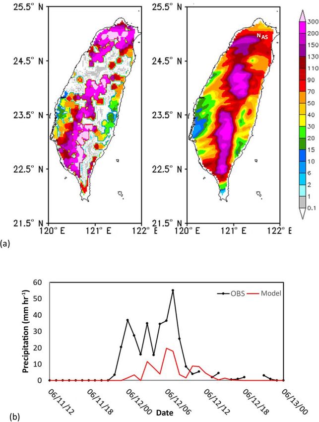
1756                                                                         I-C. Tsai et al.: Kinetic mass-transfer calculation

whereas that between ice and water vapor was adapted from            needed for condensing all supersaturated water. So, under
Ellehoj et al. (2013):                                               the saturation adjustment assumption, the kinetic effect as
                                                                     described in Eq. (5) cannot be solved fully and explicitly. In
               Rs            203.10 48 888                           mixed-phase clouds (i.e., where water and ice coexist), the
ln αl-v = ln      = 0.2133 −       +       ,                 (4b)
               Rv              T     T2                              equilibrium is maintained by assuming either water satura-
where the subscript “s” means solid phase.                           tion or ice saturation (e.g., Sundqvist, 1978) or by varying
   When the kinetic process is considered, isotopic fraction-        linearly from water saturation to ice saturation between two
ation is not only related to temperature but also factors such       specified temperature thresholds (e.g., Tiedtke, 1993). Then,
as the diffusion coefficient and water vapor concentration.          condensation on ice can be calculated following the kinetic
The calculation of kinetic fractionation during condensa-            approach, but the condensation on cloud drops still follows
tion/evaporation is based on the two-stream Maxwellian ki-           the saturation adjustment in most models. If the air is subsat-
netic equation:                                                      urated but cloud drops (or cloud ice) are present, the cloud
                                                                     drops (or cloud ice) are forced to evaporate to maintain the
dmHDO                                                               equilibrium until they are all evaporated. As the saturation
      = 4π rDHDO ρenv,HDO − ρp,HDO ,                          (5)    adjustment strategy conventionally is not applied in subsat-
  dt
                                                                     urated conditions for precipitation particles (e.g., raindrops,
where m is HDO mass in the particle, t is time, r is hydrom-         snow), it should be denoted as a partial equilibrium assump-
eteor particle size, D is the mass diffusivity in air, ρenv is va-   tion.
por density in the air, and ρp is vapor density at the particle         The kinetic effect might have significant impacts on iso-
surface. The latter two terms can be rewritten as:                   tope fractionation, thus there is a need for it to be consid-
                PHDO                       Ps,HDO                    ered in models. For example, Hoffmann et al. (1998) tried
ρenv, HDO =              and ρp,HDO = αHDO         ,          (6)    to consider the kinetic effect during deposition growth in the
               RHDO Tair                   RHDO Tp
                                                                     ECHAM AGCM model, which was developed at the Max
where RHDO is the gas constant of HDO, aHDO and Ps,HDO               Planck Institute for Meteorology. Due to the saturation ad-
are the activity and saturation vapor pressure of HDO, re-           justment assumption in ECHAM model, an effective factor
spectively, and Tair and Tp are temperatures of the air and          which is function of temperature only is used to express
particle surface, respectively. Equation (5) is for a single par-    the kinetic effect (Jouzel and Merlivat, 1984). In Wernet et
ticle, but the bulk-water microphysical schemes commonly             al. (2011), the condensation on ice is also calculated with
used in regional weather models deal with a population of            an effective factor, but the condensation on cloud drops is
hydrometeor particles (thus called bulk water). Conventional         in equilibrium fractionation. In reality, deviation from equi-
bulk-water schemes apply a mathematical function to rep-             librium is rather common in clouds, and its magnitude de-
resent the size distribution of any hydrometeor category,            pends on factors such as updraft speed and hydrometeors’
and the mathematical function is solved by knowing sev-              size spectra. These factors usually are not considered in ex-
eral bulk properties (moments) of the size distribution. The         isting models but are included in the NTU scheme.
NTU scheme is a two-moment scheme that predicts both the                Key parameters such as the HDO saturation vapor pres-
number and mass concentrations of each bulk-water cate-              sure, Ps,HDO , and diffusion coefficient, DHDO , are modified
gory, which allows better presentation of microphysical pro-         to handle HDO in the NTU scheme. The HDO saturation
cesses than the commonly used 1-moment schemes (Tau-                 pressure, which is needed for the kinetic mass-transfer cal-
four et al., 2018). In contrast to the conventional bulk-water       culation in Eq. (5), can be obtained by equating Eqs. (3) to
schemes that must assume a certain size distribution func-           (4). The derived HDO saturation vapor pressure is generally
tion, the NTU scheme derived the warm-cloud parameteri-              lower than that of H2 O, and the differences increase as tem-
zation by analyzing results from bin model simulations and           perature gets lower (Fig. 2). The mass diffusivity of HDO in
is thus rather accurate and comprehensive in microphysical           air, DHDO in Eq. (5), was obtained based on the relationship
processes, while the cold-cloud parameterization still follows       proposed by Hirschfelder et al. (1954):
the conventional approach. Another advantage of the NTU                     mair + mx
scheme is that it does not apply the “saturation adjustment”         Dx ∝             ,                                         (7)
                                                                             mair mx
strategy, as done in most global and regional models. This
saturation adjustment treatment assumes that water vapor             where x represents any gas molecule. Assuming that the pro-
and liquid (or ice) water are in thermodynamic equilibrium           portionality constants are the same for DHDO and DH2 O , one
once water (or ice) saturation is reached in non-mixed-phase         can obtain the following:
clouds (i.e., all hydrometeors are either liquid or ice). There-               mair +mHDO
fore, for models applying the saturation adjustment strategy,        DHDO      mair mHDO     ∼
                                                                           =   mair +mH2 O   = 0.9676,                          (8)
condensation is not calculated explicitly but rather by con-         DH2 O
                                                                                mair mH2 O
verting all excess water vapor into condensate, regardless of
the cloud drop size and number concentration or the time             with which we can relate DHDO to DH2 O .

Atmos. Chem. Phys., 19, 1753–1766, 2019                                               www.atmos-chem-phys.net/19/1753/2019/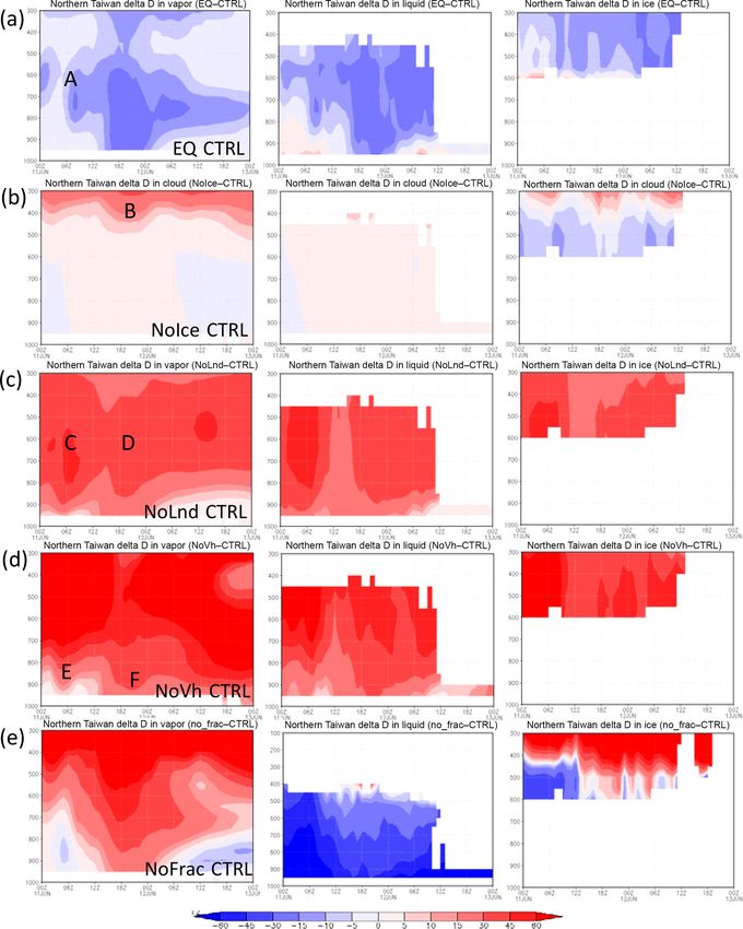
I-C. Tsai et al.: Kinetic mass-transfer calculation                                                                              1757

   In Eq. (6), the activity of water stable isotope depends on
the composition of the particle. For ice particles, the model
cannot trace the history of water stable isotope deposition
and thus cannot distinguish between the surface layer from
the inner core of the ice particles. Therefore, the water sta-
ble isotope activity of ice-phase hydrometeor is assumed
to depend on its bulk composition (i.e., assuming that it is
well mixed). In reality, however, there is no homogeniza-
tion of isotopes in ice particles due to the low diffusivities
of molecules in ice. Blossey et al. (2010), Pfahl et al. (2012),
and Dütsch et al. (2016) dealt with this problem by setting
the ice particle’s isotope ratio equal to that produced by va-
por deposition. This is an effective approach, as only the most
recently deposited ice is exposed to the vapor. However, dur-
ing evaporation the mass exchange depends heavily on the
residual composition, making the treatment rather tricky. Be-
fore a better solution is devised, this study adopted the bulk
composition approach for both condensation and evaporation
processes.

2.2   Simulation setup                                              Figure 3. Map of the model domains for the simulations in this
                                                                    study. The resolutions are 81, 27, 9, and 3 km in the outmost, 2nd,
Frontal systems are not only rich in cloud microphysical pro-       3rd, and inmost domains, respectively.
cesses but also involve air mass transitions and atmospheric
circulation. As a result, they are ideal for evaluating the rel-
ative contribution of various physical processes to isotopic        rium approach, NoIce was conducted to examine the differ-
fractionation. The case selected for this study is a frontal sys-   ences between liquid- and ice-phase fractionations, NoLnd
tem that passed through Northern Taiwan on 11 June 2012,            inspected the land–sea contrast of water vapor sources, and
with moderate to heavy rainfall from the night of 11 June un-       NoVh was for investigating the vertical exchange of isotope
til noon on 12 June. Special focus will be placed on Northern       composition between lower and upper troposphere. We also
Taiwan because of the availability of isotope measurements          conducted a blank test (NoFrac) in which isotopic micro-
for verification.                                                   physical fractionation was turned off. Descriptions of these
    The simulation domain is shown in Fig. 3. The resolution        numerical experiments is listed in Table 1.
of the coarse domain was set at 81 km, covering the region             The isotopic value for water vapor or condensates is con-
from 90 to 150◦ E and 0 to 50◦ N. The resolutions of the            ventionally expressed as δD (conventionally expressed in
nested domains were set at 27, 9, and 3 km. The innermost           ‰):
domain covers Taiwan and the surrounding ocean. Twenty-
                                                                               R

eight vertical layers were used, eight of which were below          δD =             −1 ,                                    (9)
                                                                            RSMOW
1.5 km (roughly the height of the planetary boundary layer),
with a maximum model height at 50 hPa. For the initial and          where R is the HDO/H2 O ratio in the sample, and RSMOW is
boundary conditions, we applied the National Centers for En-        the Vienna Standard Mean Ocean Water isotopic ratio (Craig,
vironmental Prediction (NCEP) final global analysis (FNL)           1961). The lower boundary condition of δD over land and
data with a 1◦ by 1◦ resolution. FNL data for wind properties       ocean are calculated by relating HDO flux to H2 O flux ac-
and temperatures were nudged into domains 1 and 2 only ev-          cording to Eqs. (3) and (4). In such a conversion, the ratio
ery 6 h for better simulation of the meteorology. The physical      Rl over land is set to be that in surface precipitation accord-
options used in the WRF model included the NTU micro-               ing to observed mean climatology in June from the Global
physical scheme, the rapid radiative transfer model (RRTM)          Network of Isotopes in Precipitation (GNIP; Johnson and
longwave and shortwave radiation scheme (Mlawer et al.,             Ingram, 2004; Rozanski et al., 1993). The obtained initial
1997), and the Yonsei University (YSU) planetary-boundary-          near-surface distribution of water vapor δD (δDV ) is shown
layer scheme (Hong et al., 2006). Cumulus parameterization          in Fig. 4a.
was turned off in the simulations.                                     The vertical distribution of initial atmospheric water sta-
    To examine different factors that control the water stable      ble isotope concentrations (Fig. 4b) was obtained from the
isotopes concentration, six simulations were conducted: the         NASA TES Aura Level 3 data (http://tes.jpl.nasa.gov/data/
control run (CTRL) used the kinetic approach for cloud mi-          products/, last access: 1 December 2018). We took the data
crophysical processes, the EQ run used the thermal equilib-         for the month of June and averaged over the years 2006–

www.atmos-chem-phys.net/19/1753/2019/                                                 Atmos. Chem. Phys., 19, 1753–1766, 2019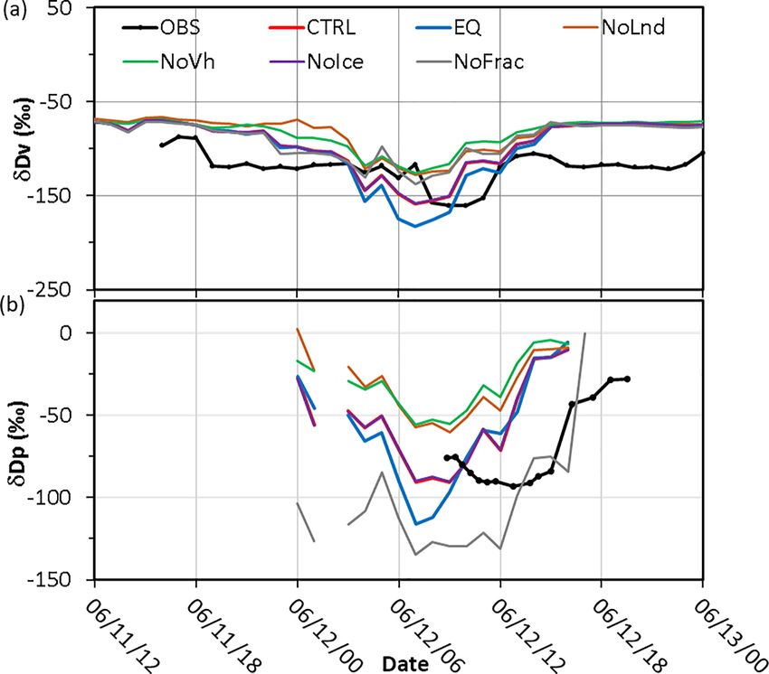
1758                                                                            I-C. Tsai et al.: Kinetic mass-transfer calculation

                                                                        Figure 5. (a) Comparison between observed (left) and simulated
                                                                        (right) accumulated precipitation (mm h−1 ) in Taiwan on 12 June
                                                                        2012. Mark N and A denotes the location of NTU and AS. (b) Sim-
                                                                        ulated (red line) and observed (black line) precipitation of 680
                                                                        (mm h−1 ) at Taipei station on 11–13 June 2012.


Figure 4. The initial distribution of water vapor δD (in ‰). (a) Sur-           + 1.134024 × QV(z).
face distribution in the coarse domain; (b) vertical profiles fitted
from satellite data (dots) of water vapor δD. Orange is for land (L),
and blue is for marine (M).                                             Note that these formulas apply only to the free troposphere;
                                                                        within the planetary boundary layers, QIV is assumed to be
                                                                        well mixed (see Fig. 4b for the full profiles).
2012. Although the concentrations of water vapor (QV) and
HDO (QIV) usually decrease exponentially with height, their             2.3   Observations
ratios (i.e., QV : QIV) vary rather linearly with height. So, for
areas over land, the vertical profile is fitted as the following:       The isotopic water vapor and rainwater δD data from 11–
                                                                        12 June 2012 were recorded using a cavity ring-down spec-

               QIVsrf                                                   troscopy analyzer (CRDS; Picarro L2120-i), following Gupta
QIV(z) =                × − 4.940699 × 10⁻⁵ × z              (10)       et al. (2009). The measurement of rainwater was conducted
               QVsrf
                                                                       on the fourth floor of the building of the Department of
         + 1.128299 × QV(z),                                            Geography, National Taiwan University (NTU, 25.02◦ N,
                                                                        121.53◦ E). The isotopic water vapor measurements were
where QIVsrf and QVsrf are the near-surface values of QIV               conducted at Academia Sinica (AS), which is about 10 km
and QV, respectively. For marine environments, the profile is           east of the rainwater collection site. The two sites are marked
fitted as                                                               as N and A, respectively, in Fig. 5a. The uncertainties in δD
                                                                     for liquid and vapor samples were found to be less than 0.3 ‰
            QIVsrf                                                      and 1.0 ‰, respectively (Laskar et al., 2014). The precision
QIV(z) =              × − 5.005261 × 10⁻⁵ × z           (11)
            QVsrf                                                       of water vapor concentration measurements made using a Pi-

Atmos. Chem. Phys., 19, 1753–1766, 2019                                                  www.atmos-chem-phys.net/19/1753/2019/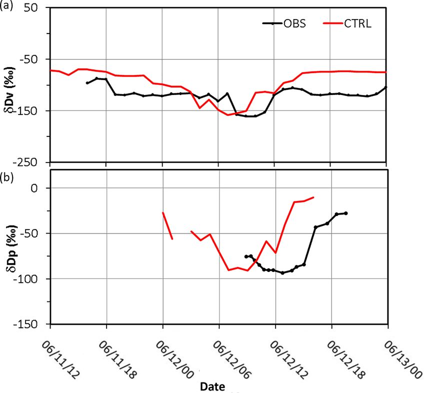
I-C. Tsai et al.: Kinetic mass-transfer calculation                                                                                  1759

Figure 6. Comparison of (a, b) simulated sea level pressure (hPa) with (c, d) the NCEP reanalysis data at 08:00 LT on 11 June (a, c) and 12
June (b, d) 2012. Frontal position is indicated by the red dashed lines.

carro CRDS is less than 100 ppmv (Crosson, 2008); this is
applicable to all of the data presented here. In addition to
these experimental data, the NCEP Reanalysis II (R2) data
and precipitation data from the Central Weather Bureau of
Taiwan (https://www.cwb.gov.tw/eng/index.htm, last access:
1 December 2018) were used to verify the simulations. Un-
fortunately, the NASA TES Aura satellite daily data during
this case are not available for verification over the studied
region.

3     Results

3.1    Model verification

Comparison of the model results with the NCEP R2 data
shows that the model captured the locations of the cold
front and associated low-pressure system reasonably well;
the front was over the East China Sea on 11 June and moved
to Taiwan on 12 June (Fig. 6). However, the simulated pre-
cipitation was generally lower than observed, especially over           Figure 7. Simulated (CTRL: red line) and observed (OBS: black
northwestern Taiwan (Fig. 5a). Additionally, the first peak in          line) (a) water vapor δDv (in ‰) at AS and (b) precipitation δDp
                                                                        (in ‰) at NTU on 11–13 June 2012.
rainfall during the early morning of 11 June (Fig. 5b), was
not obvious in the simulated results. The impact of these dis-
crepancies will be discussed in Sect. 4.

www.atmos-chem-phys.net/19/1753/2019/                                                     Atmos. Chem. Phys., 19, 1753–1766, 2019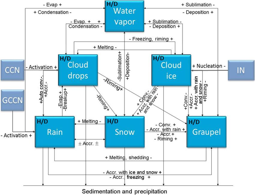
1760                                                                            I-C. Tsai et al.: Kinetic mass-transfer calculation

Figure 8. Simulated δD (in ‰) of water vapor (a, d), liquid-phase condensates including cloud and rainwater (b, e), and ice-phase conden-
sates, including cloud 697 ice, snow, and graupel (c, f) in the CTRL run at 500 hPa (a, c) and 850 hPa (d, f) on 12 June 2012.

   The observed δDV was about −90 ‰ to −120 ‰ during                   main causes for the minima. Firstly, the near-surface air in
the pre- and post-frontal periods and decreased to a minimum           the frontal zone is basically of continental origin, where the
of −160 ‰ on 12 June. The simulated δDV (from −70 ‰ to                 δDV is lower than over the oceans (cf. Fig. 4a). Secondly,
−100 ‰) values were about 20 ‰ higher than observed dur-               precipitation microphysics inside the frontal system caused
ing the pre- and post-frontal periods (Fig. 7), whereas the            a strong reduction (fractionation) in δD of hydrometeors, as
minimum δDV of −150 ‰ was slightly higher than the ob-                 can be seen in Fig. 8e and f; therefore, the evaporation of
served during the rainy period. Observation of δD in precip-           hydrometeors would produce a low δDV in the lower tropo-
itation (δDL ) was available only after 09:00 LT (local time)          sphere. The above results are in agreement with the finding
on 12 June (Fig. 7b). It decreased slightly from −70 ‰ to              of Dütsch et al. (2016), who pointed out that horizontal trans-
−90 ‰ before 16:00 LT and then recovered to around −30 ‰               port determines the large-scale pattern of water stable isotope
by the evening on 12 June. The simulated minimum is also               in both vapor and precipitation, while fractionation and ver-
around −90 ‰ but occurred a few hours earlier than ob-                 tical transport are more important on a smaller scale, near
served. The classic amount effect cannot be assessed from              the fronts. Note that the location of the hydrometeor’s δD
observations. For model simulations, the simulated δD in               minima at 500 and 850 hPa is shifted due to the structure of
precipitation (Fig. 7b) decreased with the amount precipita-           the frontal system. However, the relatively high δDV behind
tion that occurred (Fig. 5b). The negative correlation is sim-         (to the north of) the frontal system may seem a bit strange,
ilar to the amount effect in other studies. Overall, the model         as the air mass there should be of continental origin. This
captured the pattern and magnitude of changes in δD during             suggests more complicated mechanisms. Besides the water
the frontal passage reasonably well, except that the timing is         vapor source and microphysical fractionation, other factors
off by a few hours.                                                    such as the initial vertical distribution may also contribute to
                                                                       the variation in δD values. So, in order to decipher all pos-
3.2    Factors affecting isotopic fractionation                        sible controlling factors and to evaluate their relative contri-
                                                                       butions, we need to examine results from the five sensitivity
The simulated spatial distribution of δDV in Fig. 8a and d             experiments that are listed in Table 1.
shows two main zones of the minimum δDV , one over the                    The most obvious differences between the CTRL and
midlatitudes and the other over the latitudes of Taiwan. The           other simulations in terms of δD in the vapor (δDV ) and
former is mainly due to the low δD of the surface vapor                liquid (δDL ) phases at 850 hPa occurred near the front, be-
source (cf. Fig. 4a), whereas the latter is associated with            cause that is the location of the richest microphysical frac-
the frontal rainband and corresponds to the observed min-              tionation and largest contrast in air mass properties (Fig. 9).
ima shown in Fig. 7a. At a first glance, one may deduce two            Isotopic fractionation due to phase change in the CTRL run

Atmos. Chem. Phys., 19, 1753–1766, 2019                                                  www.atmos-chem-phys.net/19/1753/2019/
I-C. Tsai et al.: Kinetic mass-transfer calculation 1761
The vertical distribution of the δDV between the CTRL
and EQ runs over Northern Taiwan (121–123◦ E, 25–27◦ N)
is shown in Fig. 10a. The differences in water vapor δD at
around 850 hPa or higher prior to the passing of the front
(point A, Fig. 10a) are associated with cloud formation due
to mesoscale lifting in the warm air sector. When the frontal
system passed through Northern Taiwan in the early morning
of 12 June, low δDL extended almost down to the surface.
The δDL in the EQ run was about 30 ‰ lower than that in the
CTRL run during this period. These results suggest that the
equilibrium assumption may lead to large biases in δD for a
synoptic-scale weather system, as mentioned in other studies
(e.g., Risi et al., 2010), and kinetic calculation is crucial to
isotope modeling.
The degree of isotopic fractionation is related to tempera-
ture. As the ratio between the saturation pressure of H2 O and
HDO in different phases deviates more from unity at lower
temperatures (cf. Fig. 2), a higher degree of fractionation will
occur at lower temperatures. The significance of ice-phase
fractionation is tested with the NoIce run, for which the sat-
uration vapor pressure of ice-phase HDO was assumed to be
the same as that of the liquid phase, which leads to weaker
HDO vapor deposition on ice. The resulting differences in
the δDV are small near the surface (Figs. 9b and 10b) but
become significant at higher altitudes where the ice fraction-
ation deviates more from that of liquid. Reduced δD in the
ice phase (δDI ) can be seen immediately above the 0 ◦ C level
(Fig. 10b), causing more heavy water isotopes to remain in
the gas phase and then be transported to higher altitudes. This
results in an elevated δD in both the vapor and the ice phase.
The increase in the δDV and δDI can reach over 50 ‰ and
30 ‰, respectively, near the tropopause. Such changes may
also affect the lower troposphere, because snow and graupel
particles may fall to lower levels and bring down high δDI
water. The amount of changes due to such gravitational sort-
ing depends on whether snow and graupel were formed in the
lower or higher mixed-phase zone; the former leads to lower
δDI , while the latter increases it. However, the changes were
generally within 10 ‰. Due to the temperature dependence
of the isotopic value and the structure of the atmosphere, ig-
noring the difference between liquid- and ice-phase fraction-
ations will lead to a vertical redistribution of the isotopes.
The initial and boundary conditions are also important in
Figure 9. Difference in simulated δD (in ‰) of water vapor (left determining the isotope levels. Based on the IAEA data, pre-
panel) and liquid-phase condensates, including clouds and rainwa- cipitation δD decreases from marine to inland areas, indicat-
ter (right panel), between CTRL and other runs: (a) EQ CTRL,
ing that the water source is important in determining the ini-
(b) NoIce CTRL, (c) NoLnd CTRL, and (d) NoVh CTRL, and
tial water stable isotope content. In the NoLnd run, the initial
(e) NoFrac CTRL, at 850 hPa on 12 June 2012.
δD over land was set to be the same as that over the ocean,
and this resulted in a higher δD not only over land but also
was weaker than that calculated in the EQ run (Fig. 9a), be- in the frontal system (Fig. 9c). Ahead of the front, the vapor-
cause the isotopic compositions were not always in equilib- phase δD in the NoLnd run increased by about 40 ‰ relative
rium between the different phases in the CTRL run. That led to the CTRL run. The initial vertical distribution of the δDV ,
to slower isotopic fractionation under severe phase changes. which was based on satellite data, showed large vertical de-
cay into the free troposphere. In the NoVh run, the initial
δD in the free troposphere is assumed to be the same as that
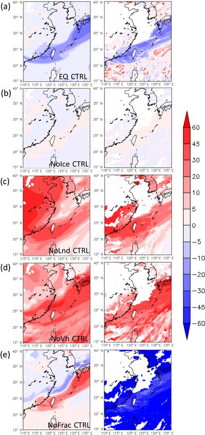
www.atmos-chem-phys.net/19/1753/2019/ Atmos. Chem. Phys., 19, 1753–1766, 20191762 I-C. Tsai et al.: Kinetic mass-transfer calculation Figure 10. Time evolution of the vertical distribution of water vapor δD (left), liquid-phase water (cloud water and rainwater; middle), and ice-phase water (including cloud ice, snow and graupel; right) over Northern Taiwan (121.123◦ E, 25.27◦ N) in different simulations: (a) EQ CTRL, (b) Nolce CTRL, (c) NoLnd CTRL, (d) NoVh CTRL, and (e) NoFrac CTRL on 11–12 June 2012. The ordinate is pressure (hPa), and abscissa is time. in the planetary boundary layer. This caused a 20 ‰–50 ‰ process does not have a significant effect on δD at lower al- overestimation of the δDV at the near surface (Fig. 9d). titudes; however, the changes in the upper troposphere are When the observed and simulated δDV values at AS and significant. The importance of microphysical fractionation is precipitation δDL at NTU are compared (Fig. 11), one can elucidated with the NoFrac run (grey line in Fig. 11), which see that the full simulation (i.e., the CTRL run, red line) yields 25 ‰ and more than 50 ‰ differences in the minimum is rather close to the observation in terms of the peak val- δDV and δDL , respectively. ues during the time of frontal passage (06:00–12:00 LT on 12 June). In contrast, the decrease in the δDV was overes- timated by 11 ‰ in the equilibrium run and underestimated 4 Discussion by 28 ‰ and 34 ‰ in the NoLnd, and NoVh runs, respec- tively. The simulated δDV in the NoIce run is rather close Combining the observations and simulations results of the to that in the CTRL run, which is consistent with the verti- water stable isotopes can be used to understand the water cy- cal profile shown in Fig. 10b, suggesting that the ice-phase cle. The observed δDV decreased after 06:00 LT on 12 June Atmos. Chem. Phys., 19, 1753–1766, 2019 www.atmos-chem-phys.net/19/1753/2019/
I-C. Tsai et al.: Kinetic mass-transfer calculation                                                                               1763

                                                                         Figure 12. Precipitation (mm h−1 ) at Nangang (dashed line) and
                                                                         Gongguan (dotted line) stations on 11–13 June 2012.

                                                                         face precipitation. In fact, most models including ours failed
                                                                         to simulate the strong precipitation over land for this sys-
                                                                         tem (Wang et al., 2016). The observed water vapor and pre-
                                                                         cipitation δD values were not in phase, and the water vapor
Figure 11. Same as Fig. 7 but for sensitivity simulations: the control   δD decreased prior to precipitation (black line in Fig. 11).
run (CTRL; red line), thermodynamic equilibrium run (EQ; blue            In contrast, the decreases in the simulated precipitation and
line), no-ice run (NoIce; purple line), no-land run (NoLnd; orange       water vapor δD were almost simultaneous, starting around
line), constant initial vertical profile run (NoVh; green line), and     03:00 LT on 12 June (red line in Fig. 11). This again sug-
no-fractionation run (NoFrac; grey line).                                gests that the model missed an earlier local convection sys-
                                                                         tem occurred during the early morning, so the simulation can
                                                                         reflect only the δD variation due to the frontal system. The
(black line in Fig. 11), much later than the onset of the pre-           simulated δDV decreased and returned to its previous level
cipitation. The observations suggested that the source of wa-            earlier than the observed δDV (∼ 03:00–10:00 LT compared
ter vapor before this time is the ocean (Wang et al., 2016)              to ∼ 07:00–13:00 LT). This also suggests that the arrival time
and that the microphysical processes related to the precip-              of the frontal system to Taipei was earlier than observed, al-
itation did not substantially affect the δDV during this pe-             though the speed of the simulated system was close to that of
riod. Model simulations can help with further understanding              the observed one, taking about 7 h to pass through Taipei.
such isotopic fractionation. The δDV on 11 June varied lit-                 Uncertainties may also exist in the observation data, as the
tle among different tests (Fig. 11), because the air mass was            vapor and precipitation measurements were taken at differ-
from nearby areas (i.e., no significant advection effect) and            ent locations, separated by about 10 km. A comparison of
no cloud microphysical processes occurred during this pe-                precipitation at different sites (Fig. 12; Nangang station is
riod. However, the water vapor δDV decreased from −80 ‰                  close to AS, and Gongguan station is close to NTU) suggests
to −100 ‰ at midnight of 11–12 June in the control run, but              that the difference in sampling locations would not signif-
not in the NoLnd run, indicating that the decreases in the δDV           icantly affect the results in this study. Another uncertainty
were due to advection of the continental air mass. When the              is the parameterization of isotopic fractionation factor α. In
front passed through during the early morning of 12 June, the            this study, the temperature dependence of αl-v and αs-v was
δDV decreased from −100 ‰ to −170 ‰ in the control run                   adopted from Horita and Wesolowski (1994) and Ellehoj et
but not in the NoFrac run (grey line in Fig. 10), indicating             al. (2013) , respectively. In most models, the formulation for
that the additional differences were caused by cloud micro-              ice and vapor by Merlivat and Nief (1967) is still used. From
physical processes. After the passage of frontal system, the             Fig. 2 one can estimate that the differences in αs-v between
δDV returned to its background level, around −80 ‰. The                  Ellehoj et al. (2013) and Merlivat and Nief (1967) are around
results of these sensitivity tests suggest that the changes in           1 % between −10 to 20 ◦ C and 4 % at −40 ◦ C; whereas the
the δDV due to cloud microphysical processes, initial vertical           differences of αl-v between Horita and Wesolowski (1994)
distribution, and lower boundary conditions are of a similar             and Merlivat and Nief (1967) are less than 1 %.
order and are all important to isotopic fractionation.                      There are also uncertainties in the treatment of microphys-
   Although the model seems to adequately reproduced                     ical processes. The isotopic value for water vapor at the lower
changes in δD in this frontal case, there are some minor                 boundary condition was assumed to be in equilibrium with
inconsistencies between the simulation results and observa-              surface precipitation in this study. Rangarajan et al. (2017)
tions. Some discrepancies originated from the meteorolog-                analyzed the isotopic ratios in water vapor from measure-
ical model itself and the initial meteorological conditions,             ments over Taipei, and they found that isotopic values were
which caused inaccuracies in the intensity or timing of sur-             not always in equilibrium. This suggests that the assumed

www.atmos-chem-phys.net/19/1753/2019/                                                     Atmos. Chem. Phys., 19, 1753–1766, 2019
1764 I-C. Tsai et al.: Kinetic mass-transfer calculation
lower boundary condition might not always be applicable for atmospheric stable isotopic composition and should be esti-
Taipei. Moreover, since the lower boundary condition can be mated from observations such as satellite data, without which
affected by fresh precipitation, the δDV might decrease after the underestimation in the decrease of water vapor δD could
the precipitation event which brings in low δDL to the soil; reach about 34 ‰ and 28 ‰, respectively. The problem in de-
however, our model does not update the surface δDV flux ac- termining the activity of water stable isotope in ice particles
cordingly. This might partially explain the discrepancy in the without knowing the inhomogeneity of chemical composi-
δDV after the frontal passage that shown in Fig. 7a. In addi- tion in the bulk ice, as mentioned at the end of Sect. 2.1, is
tion, the evaporation from the ocean is assumed to be in equi- another issue worthy of further study. To accommodate the
librium between liquid and vapor phases. This assumption different conditions between condensation and evaporation,
may also affect the simulation of δD in the model, and the it might be feasible to assume that the water stable isotope
process needs to be explicitly considered in the future study. activity is determined by the vapor phase during condensa-
Finally, whether the nonequilibrium effects are important for tion following the approach of Blossey et al. (2010), Pfahl et
the second-order isotope parameter, deuterium excess, is an al. (2012), and Dütsch et al. (2016), whereas for the evapora-
interesting subject worthy of further investigation by includ- tion process, one may assume a well-mixed bulk composition
ing the description of the δ 18 O isotope in the model. for determining the isotope activity, as done in this study. In
summary, this study suggests that a better understanding of
the relationship between water stable isotope variation and
5 Conclusions hydrological cycle can be achieved with a combination of
multiplatform observations and detailed cloud model simu-
Exploring physical processes controlling the stable isotopic lations.
composition of water, including details such as water va-
por source, atmospheric circulation, and cloud microphysi-
cal processes, is useful for understanding the water cycle. In Data availability. Data available on request from the authors.
this study, we modified the NCAR WRF model to understand
the role of different factors in the fractionation of the stable
isotopes of water. The experimental stable isotope thermal Author contributions. JP and IC designed the research. IC wrote
equilibrium data were converted into isotope saturation vapor the paper with further contributions from all co-authors. WY per-
pressure, which was then used in the two-stream Maxwellian formed the WRF simulations. MC provided measurements. JP su-
pervised the research. All authors discussed the results and con-
kinetic equation for calculating the condensation and evapo-
tributed to the final paper.
ration or deposition and sublimation of HDO, parallel to that
for H2 O. Mass conservation was also considered explicitly
for the collection processes as well as during freezing and
Competing interests. The authors declare that they have no conflict
melting. of interest.
A frontal system event was selected to reveal the complex-
ity of isotope fractionation. The model captured the location
of the front adequately, although the estimated precipitation Acknowledgements. Acknowledgment. This study was supported
was less than observed. The simulated results showed fairly by the projects MOST 105-2119-M-002-028-MY3, 105-2119-
good agreement with water vapor and rainwater stable iso- M-002-035, 106-2111-M-001-008, and 107-2111-M-001-006.
tope measurements and suggested that the decreases in water The suggestions provided by anonymous reviewers are highly
vapor δD before the front arrived in Taiwan were due to an air appreciated.
mass of continental origin. When the front passed during the
early morning of 12 June, both the water vapor sources and Edited by: Eliza Harris
the cloud microphysical processes contributed to a decrease Reviewed by: two anonymous referees
in water vapor δD, which returned to background levels after
the front had passed.
Additional sensitivity experiments showed that the ther-
mal equilibrium assumption commonly used in earlier stud-
References
ies might significantly overestimate the decrease of mean δD
by about 11 ‰, while the maximum difference can be more
Aldaz, L. and Deutsch, S.: On a relationship between air tempera-
than 20 ‰, during the precipitation event. Cloud microphys-
ture and oxygen isotope ratio of snow and firn in the south pole
ical processes, including ice-phase processes, have substan- region, Earth Planet. Sci. Lett., 3, 267–274, 1967.
tial effects on isotopic fractionation, especially on the ver- Blossey, N. P., Kuang, Z., and Romps, D. M.: Isotopic composition
tical redistribution of isotopes. Furthermore, the sensitivity of water in the tropical tropopause layer in cloud-resolving simu-
tests suggest that the initial vertical profile and the land–sea lations of an idealized tropical circulation, J. Geophys. Res., 115,
contrast in surface sources are quite important in simulating https://doi.org/10.1029/2010JD014554, 2010.
Atmos. Chem. Phys., 19, 1753–1766, 2019 www.atmos-chem-phys.net/19/1753/2019/I-C. Tsai et al.: Kinetic mass-transfer calculation 1765 Chen, J. P. and Liu, S. T.: Physically based two-moment bulkwater Horita, J. and Wesolowski, D. J.: Liquid-vapor fractionation of oxy- parametrization for warm-cloud microphysics, Q. J. Roy. Mete- gen and hydrogen isotopes of water from the freezing to the orol. Soc., 130, 51–78, 2004. critical temperature, Geochim. Cosmochim. Ac., 58, 3425–3437, Chen, S. H., Liu, Y. C., Nathan, T. R., Davis, C., Torn, R., Sowa, 1994. N., Cheng, C. T., and Chen, J. P.: Modeling the effects of dust- Johnson, K. R. and Ingram, B. L.: Spatial and temporal variability in radiative forcing on the movement of Hurricane Helene (2006), the stable isotope systematics of modern precipitation in China: Q. J. Roy. Meteorol. Soc., 141, 2563–2570, 2015. implications for paleoclimate reconstructions, Earth Planet. Sci. Cheng, C.-T., Wang, W.-C., and Chen, J.-P.: A modeling study of Lett., 220, 365–377, 2004. aerosol impacts on cloud microphysics and radiative properties, Joussaume, S., Sadourny, R., and Jouzel, J.: A general circulation Q. J. Roy. Meteorol. Soc., 133, 283–297, 2007. model of water isotope cycles in the atmosphere, Nature, 311, Cheng, C.-T., Wang, W.-C., and Chen, J.-P.: Simulation of the ef- 24–29, 1984. fects of increasing cloud condensation nuclei on mixed-phase Jouzel, J. and Merlivat, L.: Deuterium and oxygen 18 in precipita- clouds and precipitation of a front system, Atmos. Res., 96, 461– tion: Modeling of the isotopic effects during snow formation, J. 476, 2010. Geophys. Res., 89, 11749–11757, 1984. Clark, I. and Fritz, P.: Environmental Isotopes in Hydrogeology, Kurita, N.: Water isotopic variability in response to mesoscale con- Boca Raton, CRC Press, 328 pp., ISBN 1-56670-249-6, 1997. vective system over the tropical ocean, J. Geophys. Res., 118, Cole, J. E., Rind, D., Webb, R. S., Jouzel, J., and Healy, R.: Climatic 10376–10390, https://doi.org/10.1002/jgrd.50754, 2013. controls on interannual variability of precipitation δ 18 O: Simu- Laskar, A. H., Huang, J.-C., Hsu, S.-C., Bhattacharya, S. K., Wang, lated influence of temperature, precipitation amount, and vapor C.-H., and Liang, M.-C.: Stable isotopic composition of near source region, J. Geophys. Res., 104, 14223–14236, 1999. surface atmospheric water vapor and rain-vapor interaction in Craig, H.: Isotopic Variations in Meteoric Waters, Science, 133, Taipei, Taiwan, J. Hydrol., 519, 2091–2100, 2014. 1702–1703, 1961. Lee, J.-E., Fung, I., DePaolo, D. J., and Henning, C. C.: Analy- Crosson, E. R.: A cavity ring-down analyzer for measuring atmo- sis of the global distribution of water isotopes using the NCAR spheric levels of methane, carbon dioxide, and water vapor, Appl. atmospheric general circulation model, J. Geophys. Res., 112, Phys., 92, 403–408, 2008. D16306, https://doi.org/10.1029/2006JD007657, 2007. Dansgaard, W.: Stable isotopes in precipitation, Tellus, 16, 436– Lorius, C., Ritz, C., Jouzel, J., Merlivat, L., and Barkov, N.: A 468, 1964. 150 000-year climatic record from Antarctic ice, Nature, 316, Dawson, T. E. and Ehleringer, J. R.: Plants, isotopes and water use: 591–596, 1985. a catchment-scale perspective, in: Isotope tracers in catchment Merlivat, L. and Nief, G.: Fractionnement isotopique lors des hydrology, 165–202, 1998 changements d’etat solide-vapeur et liquide-vapeur de l’eau a des Dearden, C., Vaughan, G., Tsai, T.-C., and Chen, J.-P.: Exploring temperatures inferieures a 0 ◦ C. Tellus, 19, 122–127, 1967. the diabatic role of ice microphysical processes in UK summer Mlawer, E. J., Taubman, S. J., Brown, P. D., Iacono, M. J., and cyclones, Mon. Weather Rev., 144, 1249–1272, 2016. Clough, S. A.: Radiative transfer for inhomogeneous atmo- Dütsch, M., Pfahl, S., and Wernli, H.: Drivers of δ 2 H variations spheres: RRTM, a validated correlated-k model for the longwave, in an idealized extratropical cyclone, Geophys. Res. Lett., 43, J. Geophys. Res., 102, 16663–16682, 1997. 5401–5408, 2016. Pfahl, S., Wernli, H., and Yoshimura, K.: The isotopic composi- Ellehoj, M., Steen-Larsen, H. C., Johnsen, S. J., and Madsen, M. tion of precipitation from a winter storm – a case study with the B.: Ice-vapor equilibrium fractionation factor of hydrogen and limited-area model COSMOiso, Atmos. Chem. Phys., 12, 1629– oxygen isotopes: Experimental investigations and implications 1648, https://doi.org/10.5194/acp-12-1629-2012, 2012. for stable water isotope studies, Rapid Commun. Mass Sp., 27, Rangarajan, R., Laskar, A. H., Bhattacharya, S. K., Shen, C.-C., 2149–2158, 2013. and Liang, M.-C.: An insight into the western Pacific winter- Gonfiantini, R.: On the isotopic composition of precipitation in time moisture sources using dual water vapor isotopes, J. Hy- tropical stations, Acta Amazon., 15, 121–140, 1985. drol., 547, 111–123, 2017. Gupta, P., Noone, D., Galewsky, J., Sweeney, C., and Vaughn, B. H.: Risi, C., Noone, D., Worden, J., Frankenberg, C., Stiller, G., Kiefer, Demonstration of high-precision continuous measurements of M., Funke, B., Walker, K., Bernath, P., Schneider, M., Bony, S., water vapor isotopologues in laboratory and remote field deploy- Lee, J., Brown, D., and Sturm, C.: Process-evaluation of tropo- ments using wavelength-scanned cavity ring-down spectroscopy spheric humidity simulated by general circulation models using (WS-CRDS) technology, Rapid Commun. Mass Sp., 23, 2534– water vapor isotopologues: 1. Comparison between models and 2542, 2009. observations, J. Geophys. Res., 117, D05303, 2012. Hirschfelder, J. O., Curtiss, C. F., Bird, R. B., and Mayer, M. G.: Rozanski, K., Araguás-Araguás, L., and Gonfiantini, R.: Isotopic Molecular theory of gases and liquids, Wiley & Sons, Inc., New Patterns in Modern Global Precipitation, in: Climate Change in York, 1219 p., 1954. Continental Isotopic Records, American Geophysical Union, 1– Hoffmann, G., Werner, M., and Heimann, M.: Water isotope module 36, https://doi.org/10.1029/GM078p0001 1993. of the ECHAM atmospheric general circulation model: A study Sjolte, J. and Hoffmann, G.: Modelling stable water isotopes in on timescales from days to several years, J. Geophys. Res., 103, monsoon precipitation during the previous interglacial, Quat. Sci. 16871–16896, 1998. Rev., 85, 119–135, 2014. Hong, S.-Y., Noh, Y., and Dudhia, J.: A New Vertical Diffusion Skamarock, W. C., Klemp, J. B., Dudhia, J., Gill, D. O., Barker, Package with an Explicit Treatment of Entrainment Processes, D. M., Duda, M., Huang, X.-Y., Wang, W., and Powers, J. G.: A Mon. Weather Rev., 134, 2318–2341, 2006. www.atmos-chem-phys.net/19/1753/2019/ Atmos. Chem. Phys., 19, 1753–1766, 2019
1766                                                                              I-C. Tsai et al.: Kinetic mass-transfer calculation

   Description of the Advanced Research WRF Version 3, NCAR              Yoshimura, K., Kanamitsu, M., Noone, D., and Oki,
   Technical Note, 2008.                                                   T.: Historical isotope simulation using Reanalysis at-
Sturm, C., Zhang, Q., and Noone, D.: An introduction to sta-               mospheric data, J. Geophys. Res., 113, D10198,
   ble water isotopes in climate models: benefits of forward               https://doi.org/10.1029/2008JD010074, 2008.
   proxy modelling for paleoclimatology, Clim. Past, 6, 115–129,         Yoshimura, K., Kanamitsu, M., and Dettinger, M.: Regional
   https://doi.org/10.5194/cp-6-115-2010, 2010.                            downscaling for stable water isotopes: A case study of an
Taufour, M., Vié, B., Augros, C., Boudevillain, B., Delanoë, J., De-       atmospheric river event, J. Geophys. Res., 115, D18114,
   lautier, G., Ducrocq, V., Lac, C., Pinty, J.-P., and Schwarzenböck,     https://doi.org/10.1029/2010JD014032, 2010.
   A.: Evaluation of the two-moment scheme LIMA based on mi-             Yoshimura, K., Oki, T., Ohte, N., and Kanae, S.: A quantitative
   crophysical observations from the HyMeX campaign, Q. J. Roy.            analysis of short-term 18 O variability with a Rayleigh-type iso-
   Meteorol. Soc., 144, 1398–1414, 2018.                                   tope circulation model, Journal of Geophysical Research: Atmo-
Sundqvist, H.: A parameterization scheme for non-convective con-           spheres, 108, 4647, doi:10.1029/2003JD003477, 2003.
   densation including prediction of cloud water content, Q. J. Roy.     Yoshimura, K.: Stable water isotopes in climatology, meteorology,
   Meteorol. Soc., 104, 677–690, 1978.                                     and hydrology: A review, J. Meteor. Soc. Japan, 93, 513–533,
Tiedtke, M.: Representation of clouds in large-scale models, Mon.          https://doi.org/10.2151/jmsj.2015-036, 2015.
   Weather Rev., 121, 3040–3061, 1993.                                   Yurtsever, Y. and Gat, J. R.: Atmospheric waters, of IAEA, Stable
Werner, M., Langebroek, P. M., Carlsen, T., Herold, M., and                Isotope Hydrology: Deuterium and Oxygen-18 in the Water Cy-
   Lohmann, G.: Stable water isotopes in the ECHAM5 gen-                   cle, Vienna, IAEA, 210, 103–142, ISBN:92-0-145281-0, 1981.
   eral circulation model: Toward high-resolution isotope mod-           Zwart, C., Munksgaard, N. C., Protat, A., Kurita, N., Lambrinidis,
   eling on a global scale, J. Geophys. Res., 116, D15109,                 D., and Bird, M. I.: The isotopic signature of monsoon condi-
   doi:10.1029/2011JD015681, 2011.                                         tions, cloud modes, and rainfall type, Hydrol. Proc., 32, 2296–
Wang, C.-C., Chiou, B.-K., Chen, G. T.-J., Kuo, H.-C., and Liu,            2303, 2018.
   C.-H.: A numerical study of back-building process in a quasista-
   tionary rainband with extreme rainfall over northern Taiwan dur-
   ing 11–12 June 2012, Atmos. Chem. Phys., 16, 12359–12382,
   https://doi.org/10.5194/acp-16-12359-2016, 2016.

Atmos. Chem. Phys., 19, 1753–1766, 2019                                                    www.atmos-chem-phys.net/19/1753/2019/
You can also read