Land Openings on the Georgia Frontier and the Coase Theorem in the Short- and Long-Run
←
→
Page content transcription
If your browser does not render page correctly, please read the page content below
Land Openings on the Georgia Frontier and
        the Coase Theorem in the Short- and Long-Run∗
                             Hoyt Bleakley†                  Joseph Ferrie‡

                              First version: September 25, 2012
                                This version: January 9, 2014

                                                 Abstract
       The Coase Theorem, with low transaction costs, shows the independence of efficiency
       and initial allocations in a market, while the recent “market design” literature stresses
       the importance of getting initial allocations right. We study the dynamics of land-use
       in the two centuries following the opening of the frontier in the U.S. state of Georgia,
       which — in contrast with neighboring states — was opened up to settlers with a pre-
       surveyed and pre-allocated grid in waves with differing parcel sizes. Using difference-in-
       difference and regression-discontinuity methods, we measure the effect of initial parcel
       sizes (as assigned by the surveyors’ grid) on the evolution of farm sizes decades after the
       land was opened. Initial parcel size predicts farm size essentially one-for-one for 50-80
       years after land opening. This effect of initial conditions attenuates gradually, and only
       disappears after 150 years. We estimate that the initial misallocation depressed the
       area’s land value by 20% in the late 19th century. This episode suggests the relevance
       of the Coase Theorem in the (very) long run, but that bad market design can induce
       significant distortions in the medium term (over a century in this case).

       Keywords: market design, economic geography, history dependence, coordination prob-
       lem

   ∗
      Preliminary and incomplete. Comments welcome. Brian Bettenhausen and Eric Hanss were extremely
helpful in creating and processing the spatial data. The authors thank Eric Budish, Vince Crawford, Muriel
Niederle, Andres Sawicki, Alex Whalley, and seminar participants at the University of Illinois, the University
of Chicago, the NBER DAE and Market Design groups for helpful comments. We gratefully acknowledge
funding support from the Stigler Center and the Center for Population Economics, both at the University
of Chicago.
    †
      Booth School of Business, University of Chicago. Postal address: 5807 South Woodlawn Avenue,
Chicago, Illinois 60637. Electronic mail: bleakley at uchicago dot edu.
    ‡
      Department of Economics, Northwestern University. Postal address: 2001 Sheridan Road, Evanston,
Illinois 60208. Electronic mail: ferrie at northwestern dot edu.

                                                      1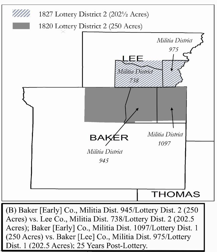
1         Introduction
The “market design” literature in economics has analyzed methods for allocating property
rights in a variety of settings (e.g., Noll 1982; Hahn 1984; McMillan 1994; Roth 2002;
Klemperer 2002; Haile and Tamer 2003; Milgrom 2011). This work has argued that getting
the initial allocation wrong can have long-run consequences for economic efficiency. This
claim that stands in stark contrast with the so-called Coase Theorem, namely that the
initial allocation of a property right should, in the absence of transaction costs, be irrelevant
to the efficiency of the final outcome. After the initial allocation is made, according to
the Coase Theorem, agents should bargain and exchange until there are no longer gains
from trade. But this outcome (as Coase, 1960, himself argued) can be long-delayed or even
thwarted entirely due to transaction costs. These costs might be prohibitively high, both
because there are real resource costs to bargaining and trading, unequal market power, or
binding information constraints, as argued by Myerson and Satterthwaite (1983).
        Theoretical results from the market-design literature have been applied to designing
allocations for radio spectrum, logging on public lands, and internet domains. (We further
review the related literature in Section 2.) Nevertheless, evidence is scarce for the long-
run impact (and whatever improvement there might be in efficiency) of a particular market
design. Compelling evidence on this question is hard to find for three reasons: (1) the usual
econometric problem that the choice of the initial allocation was endogenous; (2) the recent
adoption of many of these designs, making it impossible to evaluate long-term effects on the
efficiency of allocation mechanisms; and (3) the multiple dimensions along which particular
market designs may differ.1
        We provide evidence on the long-run impact of differences in market design from a novel
context: the opening of land for settlement on the frontier of the U.S. state of Georgia. In
the initial third of the 19th century, Georgia made almost three quarters of its total land
area available to (white) settlers in a series of eight lotteries. The historical idiosyncrasies
that led Georgia to do this are discussed in Section 3.1; suffice it to mention here that some
    1
     For example, the comparison by Libecap and Lueck (2011) between areas of the U.S. settled under
the rectangular survey (RS) system and the ancient metes-and-bounds (MB) system (in which parcels are
identified by the locations of trees, rocks, and myriad natural and man-made objects) is complicated by
differences across these areas in at least three dimensions: (1) the variation in parcel sizes (uniform sizes
under RS, no restriction on sizes under MB); (2) the shape of parcels (rectangular under RS, irregular under
MB); and (3) the presence of interstitial parcels (none under RS, potentially many under MB).

                                                     2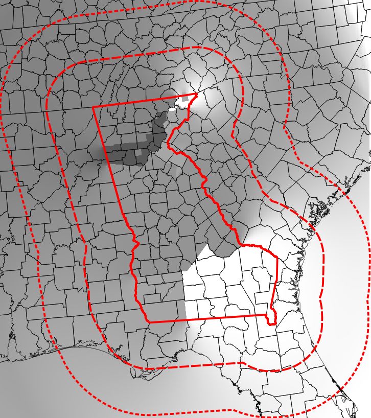
particularly egregious corruption scandals in Georgia motivated this choice for its sheer
transparency. The use of a lottery for allocation imposed two features on the market design
in this case: (a) a grid survey to demarcate parcels available to win and (b) the allocation of
property rights for all of the land to a diffuse set of owners at the moment of land opening.
This latter feature in particular contrasts with how land was opened in the rest of the region,
where land moved from public to private domain in a slow and piecemeal fashion. The waves
of the lottery mainly differed along two margins: which swath of the state was opened and
what initial farm size was imposed by the surveyors’ grid. We investigate the persistence
of these assigned farm sizes, which might reasonably be expected to be sticky. Shifting the
average farm size in a filled-out grid of farms represents a serious coordination problem.2 (In
Section 4, we discuss further the comparative market-design issues in this context.)
       Our results imply considerable persistence of the initial allocation, although not a strong
path dependence (that is, limited rather than unlimited persistence). We estimate to what
extent initial parcel size (as assigned by the surveyors’ grid) affects the evolution of farm sizes
decades after the land was opened. We find that the initial, assigned size of land lots in an
area predicts average farm size essentially one-for-one more than a half century after the land
was opened for settlement. Nevertheless, this footprint of initial conditions is more a case
of delayed adjustment rather than path dependence: the relationship between assigned and
realized farm sizes attenuates gradually, and disappears (in both a statistical and economic
sense) after 150 years. Thus, our results split the difference between the two opposing views
discussed above. On the one hand, the Coase Theorem appears to be operative in the very
long run. On the other hand, the poor market design of the lotteries induced significant costs
in the medium run, albeit a medium run that covered more than a century. The supporting
evidence for this conclusion is presented in Sections 6 and 7. (The data that we use are
described in Section 5.)
       We demonstrate this persistence using a variety of approaches and estimators. First, in
   2
     This coordination problem resembles difficulties faced in the modern allocation and re-allocation of
broadcast spectra. Milgrom (1999) discusses how markets are thin for broadcast spectra because of the
complementarities inherent in using adjacant frequency bands. While the scope of these complementarities
changes with technology, achieving optimal use of the airwaves can be difficult if all of the incumbent
broadcasters have to cooperate in reallocating who uses which frequencies. Milgrom et al. (2012) describe a
system of two simultaneous auctions, one to buy spectra and the other to sell it, as a way to coordinate the
transition to an alternate allocation of frequencies. Importantly, such a system avoids a hold-up problem
over frequencies by re-defining the (implicit) property of broadcasters as a ‘right to bandwidth’ rather than
a right to specific frequencies.

                                                     3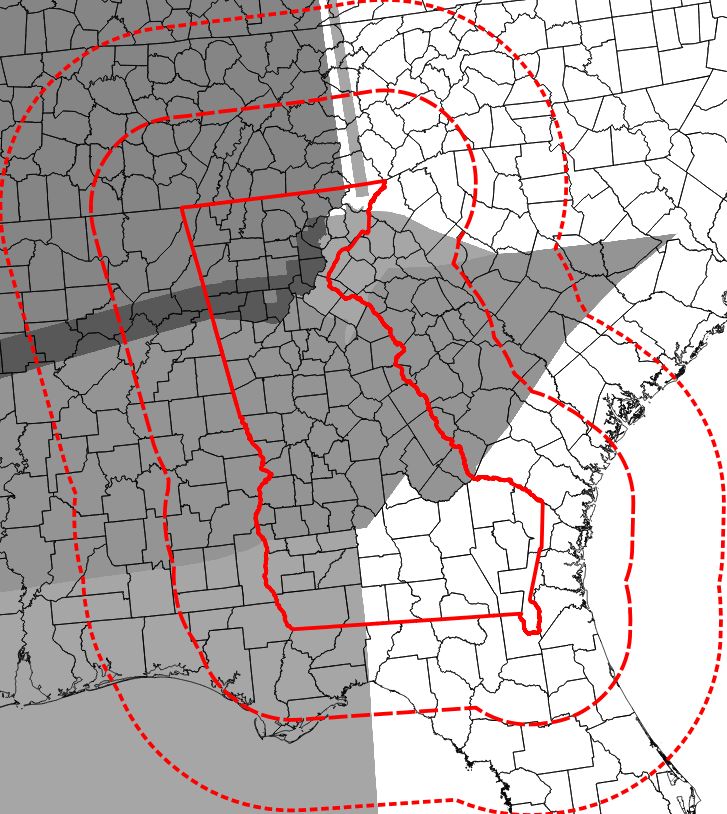
Section 3.2, we use microdata on land ownership to examine the distribution of farm sizes
decades after the land openings. We document a ‘lumpiness’ in the farm-size distribution
that maps precisely onto the initial, assigned parcel size. One to three decades after the land
is allocated, we find upwards of a third of the farms are still at the original, allocated size. Of
the remainder, almost half have sizes at some low-integer multiple or split (e.g., 2 or 12 ) of the
initial parcel size. This precise correspondence between assigned size and the actual farm-
size distribution is apparent when comparing small, adjacent areas that straddle a boundary
across which the surveyors’ grid changed its parcel size. That is, in a district opened on one
side of the boundary, the farm-size distribution several decades after land opening is ‘lumpy’
with the lumps occurring at integral multiples of the initial parcel size. On the other side
of the boundary, the distribution also exhibits lumpiness, but corresponding to that area’s
initial size.
    Next, we gauge persistence at the county level over more than a century using a difference-
in-difference design, shown in Section 6.1. We compare average farm sizes in the Georgia
Lottery Zone (hereafter “Lottery Zone” or “LZ”) to those in adjacent counties in a buffer
around the LZ (hereafter, the “Buffer Zone”). In effect, we imagine the Buffer Zone as a
pseudo-Lottery-Zone that extends past the LZ’s boundaries, and extrapolate acreage assign-
ments from the Lottery Zone to the Buffer Zone. (Details on the allocation methods in the
Buffer Zone are found in Section 3.3.) Adjoining areas in these two zones will, by and large,
share land characteristics, which allows us to use the Buffer as a comparison group. By this
assumption (which is a standard one for a difference-in-difference model), the Buffer filters
out any relationship between assigned and realized farm size arising from the endogeneity
of the assignment rule. We find that the farm sizes assigned by the surveyors’ grid are very
sticky in the Lottery Zone, over and above the (mostly attenuated) relationship in the Buffer
Zone. Further, these results are not sensitive to a variety of spatial controls, county fixed
effects, or to zooming in to sample only those areas close to the LZ’s external boundary.
    We find a similar pattern of persistence within the Lottery Zone. The variation in assigned
parcel sizes within the LZ was considerable and there were many boundaries at which parcel
sizes varied substantially. We first use a regression analysis in Sections 6.2, and show the
result is robust to a variety of spatial controls and to restricting the sample to only those
areas that were very close to a boundary where the assigned acreage changed. Relatedly, in
Section 7, we conduct regression-discontinuity (RD) tests for breaks at the boundary between

                                                4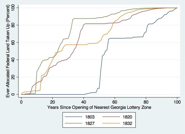
two zones with different initial assigned parcel sizes. With either estimator, we find results
that are broadly similar to those found with the difference-in-difference design.
        Finally, we show in Section 8 that the medium-run cost of misallocation was substantial.
In the postbellum years, the relationship between imputed acreage assignment and realized
farm size had gone to zero in the Buffer Zone. Taking the Buffer as a measure of the
unconstrained optimum, we then use the difference-in-difference model to impute a gap
between optimal and constrained average farm sizes in the Lottery Zone. In a auxiliary
regression, we next find that the square of the gap measure (squared for the same reason
that Harberger triangles are areas rather than lengths) predicts lower farm values. As a
check, we also find similar, albeit somewhat larger, effects of misallocation on value using
the RD model. By the middle of the 20th century, when the excess relationship between
assigned and realized farm size in the LZ has disappeared, estimates of both the gaps and the
costs of misallocation go to zero. But, in the medium term, the persistent misallocation had
a substantial cost: roughly 20% lower land values in 1880, which was already three quarters
of a century after the first lottery was conducted.

2         Related Literature
In recent years, market design has emerged as the practical counterpart to mechanism design
– they are related as engineering is to theoretical physics. Milgrom (2011) summarizes some
of the practical complications in mapping mechanism design’s findings into market design’s
real-world settings (e.g. “product definition,” “message transmission,” “incentives,” and
“linkage across markets”). An additional complication is the impact of the initial allocation
of an asset on the efficiency with which the market subsequently allocates the asset. The
concern with this issue conventionally begins with Coase (1960) and the “Coase theorem.”3
In a setting where transaction costs are present, the outcome will be shaped by the initial
distribution of the property right. This insight has been extended in a variety of ways.
    3
    McCloskey (1998) traces its provenance back through Arrow and Debreu (1954), Edgeworth (1881), and
Smith (1776), and states it simply as the proposition that “an item gravitates by exchange into the hands
of the person who values it the most, if transactions costs (such as the cost of transportation) are not too
high.” (1998, p. 368). McCloskey also asserts that Coase’s original intention was not to describe what would
happen in a setting without transaction costs but to point out that transaction costs prevent a simple first-
best solution (such as negotiation between the polluting party and those injured by pollution downstream
or downwind) from achieving the efficient outcome. In short, in the real world, the initial assignment of the
property right matters, according to Coase (McCloskey, 1998, passim).

                                                     5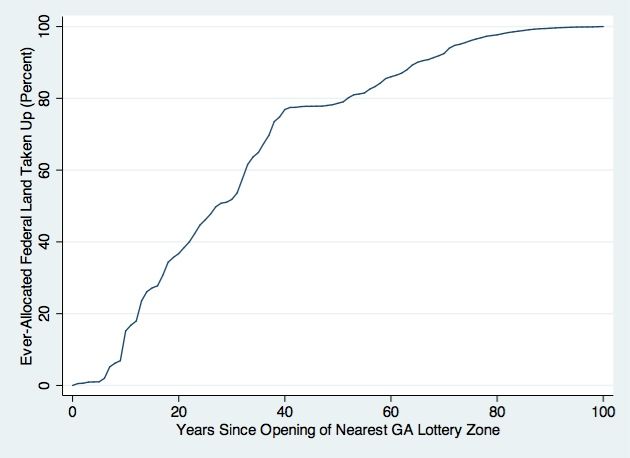
Myerson and Satterthwaite (1983) propose that information constraints may be binding
(e.g. each party may not know the other parties’ true valuations for the asset), imposing
frictions on ex post trade and preventing the achievement of the efficient allocation, while
Hahn (1984) shows how disparate market power can prevent an efficient outcome.
   The key lesson that emerges from attempts to design real-world markets in light of the
concerns raised by Coase and others on the role of the initial allocation of property rights is
that getting those rights “right” at the outset is crucial to even approximating the efficient
outcome. In the presence of transaction costs, information asymmetries, or market power,
a poor choice of initial allocation might not be remedied by the standard Pigouvian tax
on the party that is initially advantaged. Though this challenge has been recognized in
market design, the extent to which particular initial allocations lead to long-run outcomes
that depart from the efficiency has been difficult to measure in most settings.
   There are three challenges to such measurement: (1) the choice of the initial allocation
of the asset to be distributed through a particular mechanism is often endogenous (for
example, rights might be assigned to market incumbents rather than more broadly among
the set of potential market participants); (2) many market-design exercises have occurred
only recently, so long-term effects on the efficiency of the allocation mechanism in light of
the initial allocation cannot yet be observed; and (3) the assets traded in many markets
differ along multiple dimensions, complicating the identification of exactly how the initial
allocation departs from that likely to produce the efficient outcome. The particular setting
we exploit here – the distribution by lottery of land in parcels of different sizes in early
nineteenth century Georgia – allows us to overcome these challenges.
   This project is also related to a burgeoning literature, mainly in economic history, exam-
ining the persistent impact, even over spans of time as long as several centuries, of conditions
at some point in the past. Much of this work has focused on land allocation and use rules.
Libecap and Lueck (2011) compare outcomes in twentieth century Ohio where it is possible
to locate plots distributed in the nineteenth century under the ancient system of metes and
bounds immediately adjacent to plots distributed under the federal government’s rectangular
system. They find by a variety of measures that the areas with uniform, well-specified plot
boundaries at the outset were better off more than a century and a half later. Dell (2010)
examines areas on different sides of the border in Peru and Bolivia between (1) an area that
was obliged to provide labor for the silver mines from 1573 to 1812 and (2) the adjacent

                                               6
region that was not, finding higher levels of twentieth century economic development outside
the region from which labor was forcibly extracted.
Despite the insights this sub-genre has generated, we still lack a good metric by which
to assess the cost of differences in early market arrangements, whether it is the form of the
system used to survey land, the political economy of labor extraction, or the very lay of the
land. At the same time, the past differences generating these long-run outcome differences
are multidimensional, so it is difficult to isolate the differences that matter. Our work allows
us to be more precise in measuring the cost of the initial allocation, and in identifying
the mechanisms that generate outcomes nearly two centuries after the initial conditions are
observed.
Finally, our project also reflects an interest in patent law on whether the holder of an asset
(a patentee or, in our case, a lottery winner) should be required to make use of the asset in
order to secure the property right in that asset. Kitch (1977) claims that patent rights should
be distributed before the value of the thing being patented is ascertained. This arrangement
makes it easier for the patent holder to manage the development of the invention. In our
case, individuals who won parcels in the Georgia land lotteries did not immediately know the
quality of their randomly-assigned parcels and were not required to homestead them—they
could immediately sell them without so much as visiting their properties. By contrast, areas
of Alabama and Florida settled under federal land law were characterized by plots purchased
for cash and then taken up by individuals who presumably knew the quality of the asset
that they chose and, in the case of homesteaders, were obliged to remain on and improve
the land for several years. Which of these arrangements yields the more efficient outcome
(as measured by, say, average land price per acre) is a question we can investigate further
with our data.
3 Background
3.1 Origins and Nature of the Georgia Land Lotteries
The state of Georgia distributed over two-thirds of its territory to settlers in a series of land
lotteries held in the first third of the 19th century. Distributing parcels by lottery required
first delineating parcels, which was conducted by state surveyors just prior to each lottery.
7For simplicity, the surveyors imposed a uniform grid when demarcating each wave of the
land opening, and this resulted in equal-sized parcels within each wave of the lottery.
Using lotteries to allocate land on a large scale is quite uncommon and stands in marked
contrast with much of the land opening in U.S. history. Contrast a lottery with homesteading,
for example. In the case of homesteading, a large set of territory is opened for settlement, but
no specific property rights were assigned ex-ante. Instead, individuals (or heads of households
bringing their families) would go out to the open area and stake a claim. In the case of
the territories opened under the rules of the Homestead Act of 1862, the claimant would
have to spend several years working that parcel and demonstrate that the land had been
improved in order for the claim to be considered valid. Much of the interior of the original
Georgia colony (that is, the southwest side of the Savannah River watershed) was settled
in like manner through the so-called Headright System. A common alternative mechanism
elsewhere in the U.S. was the land grant, in which a large chunk of territory was given to a
single individual (often in payment for military service), who could then subdivide and sell
it. Importantly for our research design, Georgia’s neighboring states did not use lotteries to
allocate land, but rather a combination of claims and grants just discussed.
Why would the Georgia government have chosen to give out land in broad-based lotteries?
The motivation starts with two notorious corruption scandals in Georgia (and U.S.) history:
the Pine Barrens Fraud and the Yazoo Land Fraud, both of which took place in Georgia in
the 1790s. In the former episode, a number of entrepreneurs bribed and ‘packed’ local land
commissions to make and re-sell land claims (some of which were for non-existent land).
In the latter, several land companies bribed a majority of the Georgia legislature to allow
them to subdivide and sell vast stretches of land on Georgia’s then-western frontier.4 These
corruption scandals (particularly the Yazoo Land Fraud) caused a great deal of political
tumult at the time and further cast a shadow on state politics for decades to come.
Nevertheless, by 1800, only one third of Georgia’s territory had been settled (by the non-
indigenous). There was pressure on the state government to open up the rest of the state
for white settlement. As a consequence, the Native Americans’ lands were expropriated and
they were evicted from their lands in various waves throughout the first four decades of the
4
The Georgia government authorized these companies to sell land in the far West of its claimed territory,
including land in the watershed of the Yazoo River, which is currently in the state of Mississippi. (Recall
that immediately after the American Revolution, several of the original 13 colonies claimed land as far west
as the Mississippi River.)
819th century. (This particular aspect of settlement was of course not unique to Georgia.)
The tribes that were evicted from these areas were principally the Creeks and the Cherokee,
with the final set of evictions precipitating what is now known as the Trail of Tears.
When opening these newly available lands, there remained the question of how to allocate
them in an orderly fashion. The Georgian politicians of the day were mindful of the acrimony
generated by the earlier scandals. It was decided to allocate the rest of the state using a
mechanism that was as transparent as possible. As Cadle (1991) puts it,
Georgia adopted the rectangular system and the mechanism of the lottery, how-
ever, not so much as an escape from the shortcomings of the headright system
[but rather] as an indignant reaction against the two great land scandals of the
1790s—the Pine Barrens Fraud and the Yazoo Fraud. After having suffered
these experiences, the people of Georgia resolved in all future dispositions of
public lands to guard against every opportunity for fraud and corruption. (169)
The lottery system with a pre-determined grid would have been difficult to corrupt. A
typical lottery drawing was as follows. Following the surveying work, a drawing was set up by
government commission to arrange the distribution of parcels. Names of eligible Georgians
were collected from the local authorities, and each name was placed on a slip of paper.
The slips of paper were placed in one barrel. Another barrel was filled up with slips of
paper, one for each parcel available in the land opening plus enough blank slips to equalize
the number in each barrel. Both barrels were rolled around to ensure adequate mixing (or
proper randomization, in today’s parlance). The blank slips were to further increase the
transparency of the process; it was thus more difficult to increase your odds by excluding
other names from ever making it into the barrel. Having the survey before the lottery also
reduced the incentive to corrupt the parcel definitions. Even if you could influence the
surveyors to produce a parcel that was bigger and better, there would be no way to ensure
that you actually drew that parcel in the lottery. Furthermore, the parcels were very small
relative to the grants in the Yazoo episode and actually existed unlike much of the ‘land’
in Pine-Barrens episode, so there was comparatively little for a rent-seeker to steal at any
discrete step in the process. In sum, this system was hard to game, and the rewards for
doing so were limited.
The grid size for each wave was chosen in accordance with what was known about the
average land quality. For instance, the southeastern corner of the zone was dominated by
9the swampland, which was both unsuitable for agricultural use and well known by Georgians
of the era. To compensate for this, the surveyors grid for that wave of land opening was
structured to set up relatively large parcels (490 acres). On the western edge of that same
land opening wave, land quality was considerably higher, but nevertheless parcels were set
to the same size as they were around the swampy eastern part of the zone. Indeed, the
boundaries for these land-opening waves on the western side were often determined with
very little knowledge of land quality on the frontier. Each wave was typically negotiated
near the settled area between representatives of the incumbent native tribe (who may not
have actually represented the tribe at all) and functionaries of the state government. While
the surveyors laying out the grid could in theory have adjusted parcel sizes on the fly to
accommodate differences in land quality within the waves, this was not done.
Another example was the northwestern corner of the state, which was opened up following
the eviction of the Cherokees in the 1830s. This area was opened up in two simultaneous
waves. One of the waves (comprising the northern two thirds of the land opened in that
wave) saw the land divided into 160-acre parcels, because it was thought that land quality
was relatively high. The other wave was subdivided into 40-acre parcels, largely because it
was believed that the area was filled with gold deposits. (There was a modest gold rush into
this area, but it largely was a bust and was quickly was eclipsed by other discoveries farther
west, including the famous Gold Rush of 1849 in California.)
Other than differences in timing, location, and parcel size, the waves of land opening were
quite similar. Lotteries were used throughout; men satisfying minimal Georgia residency
requirement were eligible;5 and, importantly, there was no homesteading requirement. This
latter feature meant that winners of land could ‘flip’ their property just as soon as they had
won it. The announcement of the winners served to coordinate buyers and sellers into what
was a fairly liquid market in the early years of the land opening (Weiman, 1991). But, while
the single parcel itself might have been initially a liquid asset, changing a farm’s size after
the lottery would require the coordination of multiple land owners. (See Section 4 below.)
3.2 Lumpiness in the Resulting Distribution of Farm Sizes
Using microdata on farm sizes from selected areas, we see that the surveyors’ grid imparted a
significant lumpiness in the distribution of farm sizes in the 19th century. We specifically use
5
Widows and orphans were also eligible for draws. Veterans were often given extra draws.
10the county-level tax digests for Georgia, which were transcribed from Ancestry.com (2011).
The digests report landowners’ names and the acreages of their farms in the 19th century.
(Only a subset of such tax digests have survived to the present and none are fully transcribed.
We transcribed ourselves the data used in this subsection.) The Georgia property tax digests
allow us to calculate the fraction of parcels in an area that are still at the initially assigned
acreage at different dates (10–34 years) after a lottery.
3.2.1 An Example in Lowndes County, Georgia
To illustrate both these records and the apparent footprint of the surveyors’ grid, we first
turn to a representative page from the tax digests. On Table 1, we reproduce selected data
from a page of the 1830 records for Lowndes County, Georgia, which lay within a wave of
490-acre parcels and was opened by a lottery in 1820. The names of the various property
owners and the acreages of their farms are reported on the left-hand side of the table.
Each landowner’s acreage in a particular county is aggregated on the original digests. The
“ditto” lines illustrates a peculiar feature of the Georgia land taxation of the time; namely,
landowners were taxed in their county of residence on land owned anywhere Georgia. Thus,
in the next column we report the location if the land was outside of Lowndes.
We first consider the twenty farms within Lowndes. Ten years after the land opening,
seven of these farms remain at their original size of 490 acres, for example Nathan Hodge
on line three. The tax records indicate that these are the original lottery parcels rather
than some split and re-aggregation that just happened to return to 490 acres. Another nine
farms have an acreage that is either an integral multiple or an even split of 490, for example
Thomas Futch on line 14, who owns two original lottery parcels. Again, the records make
reference to the original lottery parcel designations indicating that these are assemblages of
original parcels rather than piecemeal constructions that accidentally end up being an inte-
gral multiple of 490. Thus sixteen of the twenty farms in Lowndes appear to be constrained
by the original grid size.
Next, we consider the eight farms that are outside of Lowndes County but owned by
Lowndes residents. Half of these are exactly the same size as the initial acreage assigned by
the surveyors’ grid in that other county. Of the remainder, two are double and two others a
one third split of the initial, assigned acreage. It is likely that the absentee owners were less
involved in their faraway properties, and perhaps they held them more for speculation than
11for active farming. This would dull their incentive to fine-tune their scale of production, and
thus it is less surprising that the lumpiness is so evident in this latter set of parcels. (We do
not observe on this page the farms in Lowndes county owned by those resident elsewhere, but
our inspection of other, contemporaneous tax digests reveals that absentee-owned properties
in Lowndes were almost universally 490 acres or a low-integer multiple thereof.)
Finally, in Column 7, we turn to the four parcels on the page that are apparently not so
rigidly tied to the original acreage assignment. Consider first Louis Vickers on line 24. His
landholdings are 730 acres. This is only one percent shy of being 1 12 parcels of 490 acres, and
can be readily accounted for by the occasional errors in surveying during the land opening.
The next and more interesting case is that of the Folsoms on lines 23 and 25. Neither man’s
acreage comes close to an even multiple or split, but the sum of the two farms exactly equals
2×490. This, in combination with the fact that they share a relatively uncommon surname,
suggest that the Folsom family acquired two parcels and subdivided them. Indeed, a possible
scenario is that these two men are brothers and that their father is on line 17 with another
set of two original-lottery parcels still to his name.6 The final case, shown on line 4, is
not easily rectified with the assigned grid size. Roderick Morrison owned 400 acres or 490
times 0.82, which is not a simple fraction. Nevertheless, when we look at this case of land
allocation ten years after opening, we see a very strong footprint of the initial assignment
for farm size. Of the 28 farms on this particular page, at least 26 are manifestly related to
the surveyors’ grid size or some low-integer multiple or split thereof.
3.2.2 Various Adjacent Districts Opened with Different Assigned Parcels Sizes
Even when comparing areas that are otherwise quite similar, this pattern of ‘lumpiness’ in the
distribution of farm acreages is associated with the acreage assigned at the land opening.
The tax digests identify both the Militia District (Georgia’s equivalent of a “Minor Civil
Division”) and the original Lottery District for each parcel on a county’s rolls. We compare
6
These relationships are largely confirmed by looking at records on Ancestry.com. The man on line 17,
Lawrence Folsom, was apparently of an age to have been their father. According to records on Ancestry.com,
his middle name was Armstrong and he was born in 1772. The two men, John and Randal, appear in the
1850 census again in Lowndes (on the same page), and their reported ages are both 51 years. A marriage
record for Randall notes that “Larence [sic] Armstrong Folsom” was his father. John’s eldest son in 1850 is
named Lawrence, a possible namesake for John’s father. Further, Randal’s mother was Rachael Vickers, and
thus he was probably a cousin of the man on line 24 with the 1.49×490-acre farm. The Folsom family was
apparently quite prominent in Lowndes in 1830; there are seven household heads in the 1830 census with
that surname in the county, and one of their members is the captain of the local militia.
12within Militia District/Lottery District pairs that meet three criteria: (1) they had to lie
adjacent to each other on opposite sides of a boundary between two lottery waves that used
different parcel sizes; (2) they had to have available antebellum property tax records that
allowed the same number of years from the district’s initial distribution to the year in which
parcel sizes could be observed; and (3) the property tax records for both districts had to
report individual parcel sizes and parcel designations for each parcel owned by an individual
7
(rather than just the total acreage they owned in each county where they owned land).
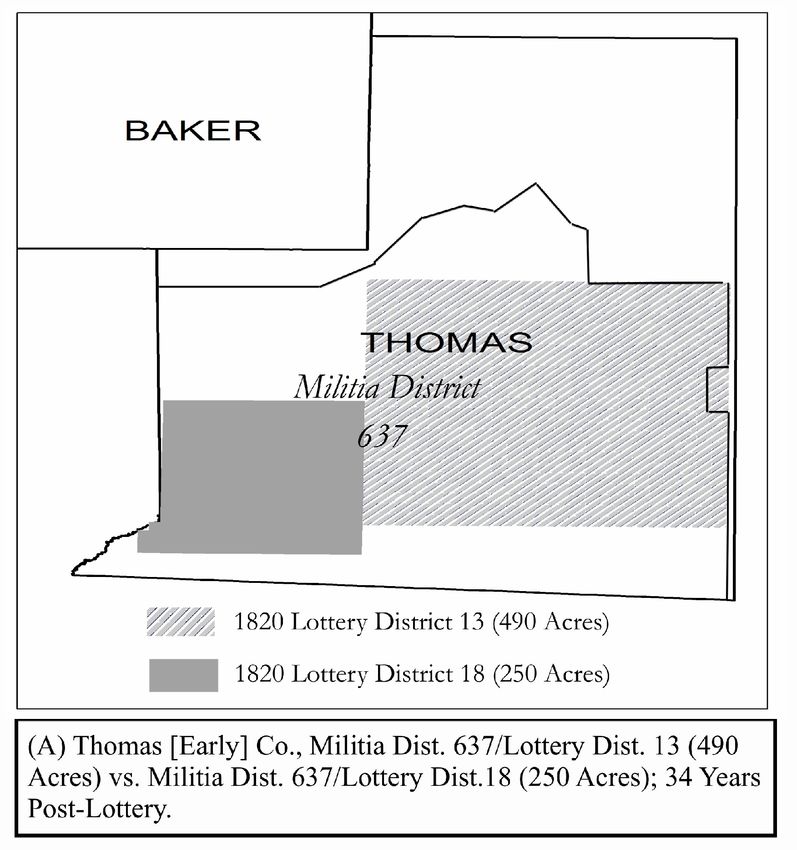
These comparability restrictions yielded exactly three pairs of Militia Districts that could
be compared. These districts are shown in Figure 1. Panel D of the Figure shows their
location within Georgia. The other panels display the location within the county or counties
of the Militia Districts and denoted their initial acreage. For example, though all of what
later became Thomas County’s Militia District 637 was distributed in the 1820 lottery, the
eastern two-thirds was originally part of Irwin County (distributed in 490 acre parcels), and
the western third was originally part of Early County (distributed in 250 acre parcels). As a
result, this Militia District, when examined in Thomas County’s 1854 tax records (34 years
after the lottery) has parcels that were originally awarded at very different sizes.
In Table 2, we find, within this narrow set, a strong correspondence between farm sizes
and the initial parcel size (or integral multiples or splits thereof). The first comparison (in
Panel A) shows that in Militia District 637 in Thomas County. This is a relatively small area
(only roughly 150 square miles), and yet parcels sizes differing by nearly a factor of two at
the time of the lottery persist in large numbers for more than three decades. In both lottery
zones that comprise Militia District 637 (the 490 acre Thirteenth District and the 250 acre
Fourteenth District), four out of every ten parcels are still at their originally assigned size
34 years later. Similar rates of parcel size persistence can be seen in Lee County’s Militia
District 975 (48 square miles), in which more than half of all parcels are either identical to
their original, unusual size (202 12 acres) or an exact multiple of it; and in Militia District
1097 in Baker County (110 square miles), where 85 percent of all parcels are either identical
to their original, size (250 acres) or an exact multiple of it.
7
Georgia’s property tax system registered taxes paid in the county where the owner resided rather than
where the property was located, so some parcels will be missed in this exercise (those owned by individuals
residing outside the counties the property tax records of which we examined).
133.3 Areas Adjoining the Georgia Lottery Zone
As discussed above, the areas surrounding the Lottery Zone did not use a lottery to assign
property rights on a grid at the moment the land was opened for settlement. Here we review
the land-allocation mechanisms used in the Buffer Zone surrounding the part of Georgia
allocated by lotteries. There were two dimensions to these allocation processes relevant for
making comparisons to the Georgia lottery zones: the mechanism through which parcels were
specified and their boundaries were defined and the mechanism through which property was
conveyed to individual landholders.
The original colonies (Virginia, North Carolina, South Carolina, and the northeastern
third of Georgia, in our case) and the lands allocated prior to 1785 (Tennessee and Kentucky,
in our case) used metes and bounds, the system of defining parcel boundaries (which could
be highly irregular) by reference to natural and man-made features of the landscape, such
as waterways, large boulders, old stone fences, stone markers placed at property boundaries,
and even large trees (Libecap and Lueck, 2011a). The situation in Alabama and Florida
is complicated by the history of French, Spanish, and/or British rule prior to becoming
U.S. territory. Grants from Spain and France did not use rectangular surveys. In the areas
settled after the lands were ceded to the U.S. and surveyed by the federal government in the
1820s and 1830s, previous claims based on Spanish and French grants were ‘carved out’ of
otherwise strictly rectangular federal survey system (Gates, 1954; Price, 1995). By the 1820s
in Alabama and by the 1830s in Florida, the remaining land was being distributed through
the federal government’s rectangular survey system, with lots of 160 acres, and also 80 acre
lots from 1866-68 (White, 1983).
The means through which title to the land reached the ultimate landholder followed
roughly the system through which parcels were defined: in the original colonies and the
areas settled prior to 1785 (all of the neighboring areas that form our Buffer Zone, except
Alabama and Florida), land was distributed through the headright system under which an
individual acquired a quantity of land proportional to the number of settlers an individual
brought to the colonies. In Alabama and Florida, however, except for the original grants
made by the French and Spanish and some headright grants in northern Florida by the
British, land was distributed through a system of cash sales, much as in the other federal
land areas opened to settlement prior to the Homestead Act (1862). After the Civil War,
some of the remaining federal land in Alabama and Florida was provided through homestead
14grants, with the requirement that the property be occupied and improved before final title
was conveyed to the grantee.
The lottery zones in Georgia thus differed from the Buffer areas in two important respects.
In the lottery zones, property rights to all parcels of land in a zone were assigned to specific
individuals at the time the lottery occurred and the area was open to settlement. In the
Buffer Zone, land was placed under the control of individuals only when those individuals
were ready to use the land, with many interstitial parcels remaining unclaimed in the decades
following settlement. At the same time, Georgia’s lottery zones had rectangular surveys with
parcels that differed in size across zones, while the neighboring states had either very irregular
parcel sizes defined under metes and bounds or (as in Alabama and Florida) a mix of a small
number of irregular parcels from grants made by Spain, France, and Britain and a large
number of rectangular parcels of uniform size (160 acres, with a small number of 80 acre
parcels granted 1866–68).
The complete record of land sales in Alabama and Florida by the federal government’s
General Land Office (GLO), initially in the Department of the Treasury, but beginning in
1848 in the Department of the Interior (P.J. Treat 1910, 136), can give us a sense of how
the Georgia lottery zones differed from adjacent areas with similar soil and climate (and as
a result, similar minimum efficient farm sizes). The Georgia system distributed all parcels
within a particular lottery zone both at once and in uniform sizes. The federal system instead
allowed purchasers to choose the location of their parcels within the townships where land was
for sale and the size of the parcels they bought, as well as when they made their purchases.
We can use the GLO federal land sale records to assess both the farm sizes that purchasers
chose and how quickly land was settled in areas adjacent to the Georgia lottery zones when
purchasers were free to determine these dimensions of their land purchases.8 By limiting our
attention to Alabama and Florida townships with twenty miles of a Georgia lottery zone, we
can infer how farm sizes and the timing of settlement might have evolved in Georgia in the
absence of the constraints on size and timing the lottery system imposed.
We extracted all 39,788 GLO records of land sales in Alabama and Georgia townships
within 20 miles of a Georgia lottery zone.9 We added together all parcels purchased by the
8
Though individual parcel purchases could be made in units as small as 40 acres, a single purchaser was
required to purchase a minimum of 80 acres total beginning with the Land Act of 1820 (Sixteenth Cong.,
First Sess., Ch. 51, 1820). The timing of an area’s settlement was also set by the date at which the GLO
surveyed and put up for initial sale that area’s federal land.
9
The selected townships are shown in Appendix Figure A. The GLO records are available online at
15same individual on the same date, resulting in 23,975 total sales. These were then grouped
by years since the opening of the nearest Georgia lottery zone. Appendix Table A shows the
fraction of federal sales that were made at exactly 160 acres. At all dates after the initial
opening of the nearest lottery zone, land sales in adjacent Alabama and Florida townships
occurred at a variety of sizes. For example, in the Alabama townships within twenty miles of
the Georgia 1832 zone wth its 160 and 40 acre parcels, less than a fifth of sales through 1842
were at 160 acres. This suggests that, in the absence of the uniform parcel size constraint
imposed by the Georgia system, settlers would have chosen the majority of the parcels they
purchased at sizes different from the size imposed in Georgia.
The same records can be used to determine how quickly land similar to the Georgia
lottery zones would have been settled if individuals could choose when to purchase land and
the size parcels in which they made those purchases. Appendix Figure B shows, at each date
since the opening of the nearest Georgia lottery zone, how much of the land ever sold had
been purchased in Alabama and Florida townships within twenty miles of Georgia. Panel A
shows that, across all these townships, no more than two fifths of the land ever purchased had
been bought within twenty years of the opening of the adjacent lottery zone. The fraction
purchased does not reach eighty percent until fifty years after the opening of the adjacent
lottery zone. This suggests that the settlement of Georgia in the areas distributed by lottery
could have taken five or more decades if the land had not been distributed as it was all at
once.
4 Market-Design Issues
In this subsection, we discuss the possible difficulty of adjusting farm sizes, particularly in
the Lottery Zone of Georgia, where the land grid was fully allocated to a diffuse set of owners
from the outset.
For our purposes, the main issue in designing the land opening is whether it could get
close to setting an optimal farm size at the moment of opening, or at least whether it could
facilitate the transition to optimally sized farms later on. In a frictionless world, the design
and outcome of the lottery has purely distributional consequences. Such is the insight of
the Coase Theorem. If cheap enough, transactions will occur until the optimal distribution
http://www.glorecords.blm.gov/search/.
16of farm sizes and the efficient mapping of farmers to plots are obtained. How much and for
how long costs of transaction might impede this march to efficiency are nonetheless empirical
matters.
These land openings differ from some other contexts to which market design is applied.
First, one side of the market (the land lot) lacks agency or preferences with respect to
its owner. This is a less important difference in that (a) the farming production function
is analogous to preferences over the match and (b) the government itself might prefer an
efficient use of the land, which would not necessarily occur given the absence of prices at
the initial allocation. This logic is similar in the case of allocating cadaveric organs for
transplantation. Second, while land lots are by definition discrete (like kidneys), there is a
continuum of ways to partition land into lots (unlike kidneys). In this sense, the allocation
of land is like a two-dimensional version of the allocation of broadcast spectra, a case that
has received some attention in the market-design literature (e.g., McMillan 1994; Milgrom
1999).
Relatedly, much of the market design literature is focused on the issue of what could
be called “strategy-proofness,” meaning that agents would not wish to misrepresent their
preferences during the process. At a very basic level, the land lottery easily passes this test
because the space of signals is so limited: (i) register or not for the lottery; (ii) make a
claim or not if you should happen to win. (As discussed above, it was designed to be hard
to manipulate.) Nevertheless, strategy-proofness is a goal not for its own sake, but rather
because ex post trade is costly.
The land-reallocation problem is complicated by the fact that the assets fill out a two-
dimensional space (the Earth’s surface). Exploiting scale economies in agriculture typically
requires the land of a given farm to be contiguous, which creates strong complementarities
among neighboring pieces of land. In the case of individual land lots, trade is costly, although
not prohibitively so, especially when such costs can be amortized over a long enough time
horizon. (This is not to say that the costs are trivial. Information asymmetries could be
particularly acute in that there is much that is hard to observe about land quality and land
improvements.)
Even if Georgia politicians somehow got the optimal farm size correct at the initial
opening, over time changes in prices and technology would cause this optimum to drift.
Furthermore, the fact that the grid restricted parcel sizes to be homogeneous within a wave
17would imply that some areas (such as the non-swampy areas of the wave mentioned above)
would be wrong from the outset.
Consider the coordination problem involved in shifting an area with an already-allocated
grid to a different average farm size. The simplest case is when the optimal farm size drops
by some integral factor N . If so, the existing owners can just subdivide into N lots. A more
complicated case would be if the optimal farm size goes up by some integral multiple M . To
achieve these new gains from scale, M neighbors would need to get together and negotiate
which one of them buys out the rest. This situation presents a classic “holdout” problem
in that any one of those M neighbors could threaten to sink the deal unless he receives an
outsized share of the surplus.
A more realistic and still more complicated case would arise if the optimal farm size
changed more slowly over time, say by a few percent in a decade. Consider first the simple
example with bilateral negotiation. In order for my farm to get α bigger, my neighbor’s has
to get α smaller. But a quick analysis of the optimization problem illustrates why this would
be difficult to negotiate. Suppose that my farm and my neighbor’s farm are symmetric,
and let π ∗ (x) be the profit function (profits after optimizing the input mix), conditional
on farm size x. We assume the usual conditions on the profit-maximization problem such
d2 π ∗
that there exists an optimal farm size x∗ and that dx2
< 0 in a neighborhood around x∗ .
Define x̃ ≡ x − x∗ , the deviation from the optimum, and π̃(x̃) ≡ π ∗ (x) − π ∗ (x∗ ), the loss
associated with not being at the optimum. The quadratic derived from a second-order Taylor
approximation of π̃ at x̃ = 0 is
π̃(x̃) ≈ ax̃2 + bx̃ + c
By construction of π ∗ , c = 0 and a > 0. By virtue of x∗ being optimal, b = 0. Assume for
simplicity that both farms have an x̃ = α. My gain from moving from x̃ to 0 is approximately
aα2 , while my neighbor’s loss if doubling his x̃ is (a(2α)2 − aα2 ) = 3aα2 , which is greater
than my potential gain by a factor of 3. Thus, there are no gains from trade, at least local
to x∗ (that is, for |α|
x∗ ), because my moving closer to the optimum raises my value less
than what it costs him to move the same amount away from the optimum.10
Allowing for negotiation among more (symmetric) neighbors does not necessarily help,
however. The curvature of the optimization problem means that the gains from getting
10
Note that this is related to Harberger’s notion that the loss associated with being distorted farther from
the optimum is second order, and thus grows like the square of the deviation.
18closer will be smaller than the losses from getting farther away. For α large enough, all of a
farm’s neighbors could ‘carve up’ the farm in between. But this might be hard to pull off in
such a thin market, again with the possibility of holdout problems.
None of this would be a problem if there were no need for a farm to be a contiguous
piece of property. This would break the complementarity amongst neighbors, and as a result
the market for added farmland would be quite thick from the perspective of any one farmer
trying to expand. There were indeed some discontiguous plantations in the antebellum South
(Ransom and Sutch, 1977). This was likely a work-around if the planter was unable to acquire
an adjacent parcel of land, and may be an exception that proves the rule in that the planter
was taking on additional transportation costs and perhaps reducing the economies of scale
associated with more land rather than being ‘held up’ by the owner of the desired adjacent
parcel.
Politicians of the era were already paying attention to what would be regarded as market-
design issues today. For example, even though the vast majority of the territory was allocated
in a rectilinear grid, town and university sites were preselected because it was deemed easier
to do so ex ante than to assemble them later from various owners (Holder, 1982). This idea
was also used by the Public Land Survey System (PLSS) that was used to allocate land in
most of the central part of the U.S.
The choice to use a lottery itself indicated taking stands on a market-design question.
An even more transparent alternative would be to chop up each wave of land into n pieces
if n persons register for the lottery. In the case of the Cherokee Land Lottery of 1832, the
lottery for 160-acre parcels was oversubscribed by a factor of nine. Chopping up the land
would have resulted in parcels of approximately 18 acres, which would have been well below
what would have been considered the minimum efficient scale of the time. For any of this
land to have been useful, therefore, such an initial allocation would have required a massive
amount of land swapping and would likely have been hampered by coordination problems in
the attempt to assemble large, contiguous parcels.
The state of Georgia also published lists (for example, Smith, 1838) to facilitate land
claims and reduce transaction costs. These lists identified the lottery winners by names
and reported both their parcel won and their county/township of residence at the time of
the lottery. The point of the list was to not just announce the winners, but also connect
potential buyers and sellers. There are various anecotes of prospective buyers going to
19great lengths to find the winner of particularly valuable (and complementary) plots. Indeed,
Weiman (1991) presents evidence that the lottery increased liquidity in land markets in the
immediate aftermath of each land opening. Nonetheless, while the lottery may have increased
the degree of ‘flipping’ of lots in the early years, it is less clear that it had much effect on
the structure of land lots imposed by the surveyors’ grid. A survey of one county in the
antebellum years showed the vast majority of land transactions occurring for lots that were
precisely the same size as those from the surveyors’ grid. While this may have represented
consolidation of lots into plantations, it did not reflect a change in the fundamental grid
structure.
Decades after the land opening, it may have been more difficult to locate a lot’s owner,
which presents challenges to making marginal changes in farm size on a fully allocated grid.
Using the state-disseminated lists to find a winner who wanted to sell might be easy in the
lottery’s immediate aftermath, but those lists would become dated rather quickly in a period
of high westward migration. Nevertheless, the low cost to claim land winnings motivated
most lottery winners to take formal possession of their lot. But even owners who undertook
to develop their lot may have become impossible to find if they subsequently abandoned
their land.11 Roger Ransom (2005) dubbed this period the era of “walk away farming,” in
which it was commonplace for farmers to simply leave their land in response to bad shocks.
Obviously you cannot negotiate with a neighbor that you cannot find, and such ‘walk away’
neighbors would retain de jure ownership of their lot for some time. A farmer who wanted
to expand on to this abandoned land could do so with some hope of eventually acquiring
title, but this was not without risk.
5 Data
In the present study, we trace out the relationship between initially assigned parcel size and
land outcomes over time. This requires, broadly defined, two types of data. The first type
consists of spatial data. We construct information on the location and characteristics of each
11
In relation to the question of what fraction of winners actually took up residence on the long-term basis,
we estimate in other work (Bleakley and Ferrie, 2013) that, 18 years after winning in the 1832 Cherokee
Land Lottery, only two percentage points more winners resided in the Cherokee area, compared to the control
group of lottery losers. As to the immediate aftermath of the allocation, Weiman (1991, page 840) examines
tax records in four counties opened up by 1821 and 1827 lotteries and estimates that only 12% of the land
owners had won the parcel that they occupied.
20wave of land opening, and we link this information spatially to data on administrative units
(counties and minor civil divisions). The second type of data is aggregate information (most
prominently average farm size and farm value), which we relate to the assigned parcel size
from the land opening. Below we discuss the sources, construction, and linkage of these data
in turn.
We code the boundaries of each land-opening wave of the lotteries using historical maps
and textual sources. Our principal reference for the location of these boundaries starts with
a map of Georgia with details on land-opening districts (Hall, 1895) and a book detailing
the history of land surveying in Georgia (Cadle, 1991). For comparison, county boundaries
for each census year are drawn from the National Historical Geographic Information Sys-
tem (NHGIS, Minnesota Population Center 2004) and major rivers in the “Streams and
Waterbodies” map layer, from NationalAtlas.gov.
We started with a geo-referenced version of Hall’s map. From there, and with textual
confirmation from Cadle’s book, we identified the vast majority of district boundaries in
either the spatial data for rivers or for historical county boundaries. (As it happened,
the footprint of land-district boundaries persisted in the county boundaries for at least a
decade and in some cases to the present day.) In a few additional cases, a district boundary
was a simple straight-line extrapolation of a linear county boundary. The majority of the
additional boundaries not identified with the above methods were in the northwestern corner
of the state. Serendipitously, we were able to find scanned and geo-referenced versions of the
original surveyors’ maps for that area.12 For the remaining boundary segments, we relied on
textual descriptions in Cadle (1991), which were occasionally supplemented with information
on features from USGS Quad maps (for example, for the location within Wilkinson and
Laurens Counties of Turkey Creek, a stream that was too minor to appear on the ‘rivers
and streams’ file). As with any spatial data set, there are no doubt errors in the exact
placement of each feature. Note nevertheless that such errors are unlikely to be important
because (a) the waves of land opening were quite large and (b) we are mostly working with
data on counties, which are large relative to the errors that might be reasonably expected
in our coding of the boundaries. In what follows, we refer to the area within Georgia that
was opened up via lotteries as the “Lottery Zone” or LZ.
Across the Lottery Zone, waves differed not only as to when and where the land was open,
12
These correspond to the maps found in Smith (1838), and were downloaded from data.georgiaspatial.org.
21You can also read