Land surface temperature from Ka band (37 GHz) passive microwave observations
←
→
Page content transcription
If your browser does not render page correctly, please read the page content below
JOURNAL OF GEOPHYSICAL RESEARCH, VOL. 114, D04113, doi:10.1029/2008JD010257, 2009

Land surface temperature from Ka band (37 GHz) passive
microwave observations
T. R. H. Holmes,1 R. A. M. De Jeu,1 M. Owe,2 and A. J. Dolman1
Received 11 April 2008; revised 21 November 2008; accepted 17 December 2008; published 25 February 2009.

[1] An alternative to thermal infrared satellite sensors for measuring land surface
temperature (Ts) is presented. The 37 GHz vertical polarized brightness temperature is
used to derive Ts because it is considered the most appropriate microwave frequency for
temperature retrieval. This channel balances a reduced sensitivity to soil surface
characteristics with a relatively high atmospheric transmissivity. It is shown that with a
simple linear relationship, accurate values for Ts can be obtained from this frequency, with
a theoretical bias of within 1 K for 70% of vegetated land areas of the globe. Barren,
sparsely vegetated, and open shrublands cannot be accurately described with this single
channel approach because variable surface conditions become important. The precision of
the retrieved land surface temperature is expected to be better than 2.5 K for forests and
3.5 K for low vegetation. This method can be used to complement existing infrared
derived temperature products, especially during clouded conditions. With several
microwave radiometers currently in orbit, this method can be used to observe the diurnal
temperature cycles with surprising accuracy.
Citation: Holmes, T. R. H., R. A. M. De Jeu, M. Owe, and A. J. Dolman (2009), Land surface temperature from Ka band (37 GHz)
passive microwave observations, J. Geophys. Res., 114, D04113, doi:10.1029/2008JD010257.

1. Introduction                                                        TIR measurements under clear skies. The TIR measurements
                                                                       usually need a correction for atmospheric constituents like
  [2] Land Surface Temperature (Ts) is defined as the ther-            water vapor, aerosols and particulate matter, and no obser-
modynamic temperature of the uppermost layer of the Earth’s            vations are possible under clouded conditions. The latter is an
surface. Ts is an important variable in the processes control-         important limitation because on average 50% of the land
ling the energy and water fluxes over the interface between            surface is covered by clouds [Rossow et al., 1993].
the Earth’s surface and the atmosphere. For continental- to              [4] Passive microwave observations can be an alternative,
global-scale modeling of these land surface processes there            or an addition to TIR sensors, for measuring Ts, in particular
is need for long-term remote sensing – based Ts for validation         at the Ku band (18 GHz) or Ka band (37 GHz). Observations
and data assimilation procedures. Furthermore, Ts is a key             within these channels are typically divided in horizontal and
input variable in numerous soil moisture retrieval method-             vertical polarization. The vertical polarized channel is better
ologies from space observations [e.g., Kerr et al., 2001; Owe
                                                                       suited for temperature sensing than the horizontal channel
et al., 2001; Njoku et al., 2003; Verstraeten et al., 2006].
                                                                       because it is less sensitive to changes in soil moisture at
  [3] Continental- to global-scale modeling requires Ts to be
                                                                       incidence angles of 50– 55°. Of these two microwave bands,
an area averaged value for each model grid square, typically
                                                                       Ka band is the more appropriate frequency to retrieve Ts
sized between 0.5 and 2.0°. Remote sensing is ideally suited
                                                                       because it balances a reduced sensitivity to soil surface
to give area averaged values at this spatial resolution.
                                                                       characteristics with a relatively high atmospheric transmis-
Commonly used global Ts products are derived from thermal
                                                                       sivity [Colwell et al., 1983]. The sensitivity to soil surface
infra red (TIR) sensors that are integrated in many satellite
                                                                       parameters is lower at Ka band than at Ku band because
systems (e.g., polar orbiting AQUA, as well as geostationary
                                                                       vegetation scatters the surface emission more effectively. As
platforms like GOES and METEOSAT). The spatial resolu-
                                                                       a result, even a thin vegetation cover is opaque to TB,37V
tion of TIR measurements ranges from 1 to 5 km for polar
                                                                       emission. The use of TB,37V for deriving Ts is limited by snow,
orbiting satellites to 50 km for geostationary platforms.
                                                                       frost, and frozen soil, as these conditions have a large effect
Assuming that the land surface emissivity is known, the
                                                                       on the emissivity that cannot easily be parameterized. The
actual temperature of the land surface can be derived from
                                                                       atmosphere appears more opaque at Ka band than at Ku band,
                                                                       resulting in an effect of the atmospheric temperature. Also,
   1                                                                   rain bearing clouds or active precipitation with droplets close
     Department of Hydrology and Geo-Environmental Sciences, Vrije
Universiteit, Amsterdam, Netherlands.                                  to the size of the wavelength (8 mm for 37 GHz) will scatter
   2
     Hydrological Sciences Branch, NASA Goddard Space Flight Center,   the microwave emission [Ulaby et al., 1986]. TB,37V obser-
Greenbelt, Maryland, USA.                                              vations have a spatial resolution of 10 to 25 km, which is
                                                                       somewhat higher than the resolution of current global land
Copyright 2009 by the American Geophysical Union.                      surface models, but lower than most TIR measurements.
0148-0227/09/2008JD010257

                                                                 D04113                                                       1 of 15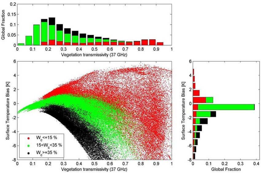
D04113                       HOLMES ET AL.: LAND SURFACE TEMPERATURE FROM KA BAND                                          D04113

                                                                     between the Ts and the measured TB,37V at the top of the
                                                                     atmosphere. On the basis of these simulations, a single
                                                                     linear relationship between Ts and TB,37V is derived, that can
                                                                     then be applied globally. Comparisons to field data are used
                                                                     to validate this approach.

                                                                     2. Materials and Methods
                                                                     2.1. Ground Measurements
                                                                       [8] FLUXNET is a network of meteorological towers
                                                                     spanning the entire globe [Baldocchi et al., 2001]. From
                                                                     this database 17 sites are selected that have good records of
Figure 1. Operating years of microwave radiometers in                longwave radiation, sensible heat flux and air temperature
orbit. The SSM/I sensor has been on several overlapping              for the year 2005, with a temporal resolution of a half hour.
DMSP missions, and the AMSR-E sensor is included in the              Secondary variables for this analysis are net radiation and
AQUA and WINDSAT missions.                                           wind speed. These sites represent a variety of vegetation
                                                                     types and climates (see Table 1). The dominant IGBP land
  [5] Besides these theoretical considerations, there is an          cover class for the surrounding 0.15° grid box is based on
important additional advantage to using either Ku band or            the MOD12Q1 Land Cover Product [Belward et al., 1999].
Ka band and that is that these channels have been a constant         The reader is referred to http://www.fluxnet.ornl.gov for a
part of satellite microwave missions since the late 1970s.           detailed description of all sites.
Continuous measurements of TB,37V are now available from               [9] As discussed previously, Ts is the integrated temper-
1978 to the present from the Scanning Multichannel Micro-            ature of all the land surface covers in a given radiometric
wave Radiometer (SMMR), the Special Sensor Microwave                 footprint. It follows then that it cannot be measured at a
Imager (SSM/I), the TRMM Microwave Imager (TMI) and                  single point, nor is it easily estimated by multiple observa-
the Advanced Microwave Scanning Radiometer (AMSR-E),                 tions of the soil and canopy surfaces. One way to address
see Figure 1. These radiometers are all on polar orbiting            this problem is by comparing Ts with the emitted longwave
satellites with global coverage, except the TMI that has an          radiation. The longwave flux is a direct function of the
equator orbiting path between 40° north and south. In the            physical temperature of the land surface, and like Ts, is
future, the current missions will be continued and expanded          representative of all the radiating surfaces in the sensor’s
(TRMM by the Global Precipitation Monitoring mission                 view. The benefit of this approach is that no temperature
(GPM) Microwave Imager, AMSR-II on the GCOM-W,                       conversions need to be made to compare temperatures from
and a new Microwave Radiometer Imager (MWRI) is                      different depths. Instead, the longwave emissivity (e) must
planned on the Chinese FY-3).                                        be determined for each site separately to calculate the land
  [6] At this point it is important to qualify how Ts is             surface temperature, now denoted TLW. The procedure to
defined. The depth of the surface layer that Ts refers to            determine e is outlined below.
depends on the sensor and the composition of the land surface          [10] Although the use of the longwave flux makes it easier
in the sensor footprint. For bare surfaces, Ts represents the soil   to compare the satellite derived temperature with ground
temperature at a shallow depth that depends on view angle,           measurements, the footprint of the flux tower measurement
wavelength, and the surface characteristics (e.g., roughness,        remains much smaller than that of the satellite. Heterogeneity
wetness, and soil texture). This thermal sampling depth is           within the satellite footprint can therefore cause a bias
50 mm for TIR frequencies, and at 37 GHz between 1 mm               between the two measurements, if the location of the flux
for a wet soil and up to 10 mm for a dry soil [Ulaby et al.,         tower is not representative for the 25  25 km area. For this
1986]. When the surface is covered with vegetation, Ts               reason the satellite derived land surface temperature will
represents the canopy surface temperature. In this paper, Ts         principally be validated against the ground measurements in
refers to the area weighted average of the temperatures of the       terms of correlation R2 and standard error of estimate (SEE),
various land covers within a specific scene. As will be shown,       and not in terms of bias.
at 37 GHz the vegetation is relatively opaque, and for most          2.2. Longwave Emissivity
of the Earth (60%) Ts will effectively represent the vegeta-
tion canopy temperature.                                               [11] The relationship between outgoing longwave radia-
  [7] In the past, several authors used the 37 GHz signal to         tion (FLW,up) and longwave surface temperature, denoted
derive surface temperature for different well defined study          TLW, is based on the Stefan-Boltzmann law, according to:
sites and observed a strong linear relationship between TB,37V                                           4
and Ts [e.g., Owe et al., 2001; Owe and Van de Griend, 2001;                                FLW ;up ¼ esTLW                     ð1Þ
De Jeu and Owe, 2003]. Other authors have tried multi-
frequency approaches [e.g., Fily et al., 2003], but these            where e is the broadband emissivity for the entire TIR
techniques have been more difficult to apply globally. This          spectral region and s is the Stefan-Boltzmann’s constant
paper will continue with the single frequency approach and           (s = 5.6697  108 Wm2 K4).
examine the potential of 37 GHz passive microwave obser-               [12] According to Penman [1948], the sensible heat flux
vations for deriving land surface temperature at global scales.      (H) can be described as H = CDT, with C representing
Simulation studies are used to test the theoretical influence        vegetation-dependent parameters and boundary conditions.
of the most important           rs that affect the relationship      DT is the temperature difference between the land surface

                                                               2 of 15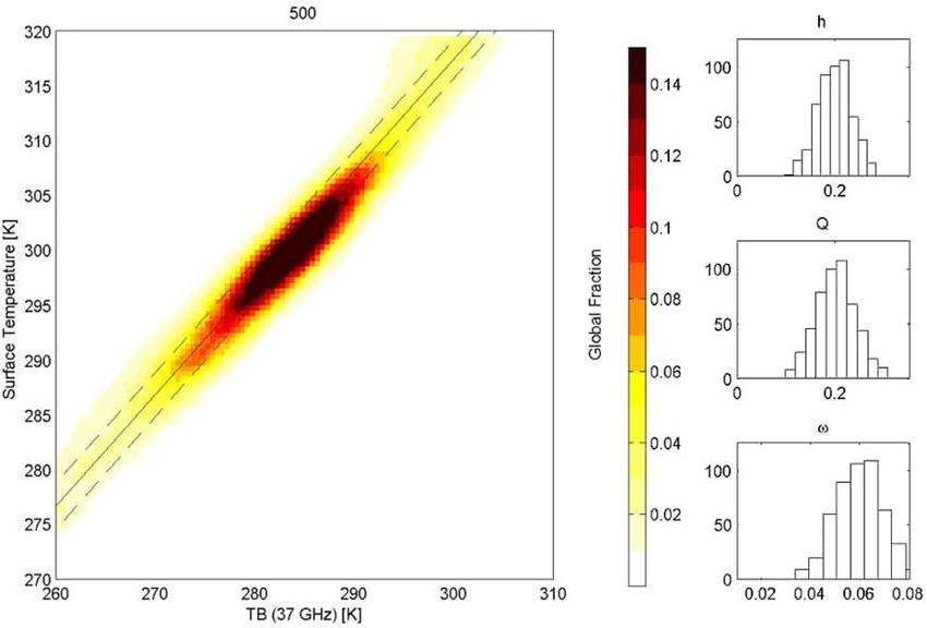
D04113                             HOLMES ET AL.: LAND SURFACE TEMPERATURE FROM KA BAND                                                    D04113

Table 1. Geographical Location, IGBP Vegetation Class, and LW Emissivity for 17 Field Sites
ID               Site Name              Latitude Longitude        Vegetation Class at Site          Vegetation Class 0.15°         Emissivity at Site
                                                             Low-Vegetation Group
A       Arizona,a US                    31.59°N 110.51°W grasslands                           grasslands                                 0.946
B       Fort Peck Montana,a US          48.31°N 105.10°W grasslands                           cropland/natural vegetation mosaic         0.961
C       Brookings South Dakota,a US     44.35°N 96.84°W croplands                             croplands                                  0.971
D       Bondville Illinois,a US         40.01°N 88.29°W croplands                             croplands                                  0.961
E       Bondville comp. Illinois,a US   40.01°N 88.29°W croplands                             croplands                                  0.938
F       Cabauw,b NL                     51.97°N 4.93°E   croplands                            croplands                                  0.995
G       Gebesee,c DE                    51.10°N 10.91°E  croplands                            croplands                                  0.987
H       Mitra II,d Evora, PT            38.54°N 8.00°E   cropland/natural vegetation mosaic   cropland/natural vegetation mosaic         0.980

                                                                High-Vegetation Group
I       Ozark Missouri,a US             38.74°N   92.20°W    deciduous broadleaf forest       cropland/natural vegetation mosaic         0.970
J       Morgan Monroe Indiana, US       39.32°N   86.41°W    deciduous broadleaf forest       deciduous broadleaf forest                 0.995
K       Collelongo beech,e IT           41.85°N   13.59°E    deciduous broadleaf forest       mixed forest                               0.960
L       Mehrstedt1,f DE                 51.28°N   10.65°E    mixed forest                     croplands                                  0.989
M       Loobos,g NL                     52.17°N   5.74°E     evergreen needleleaf forest      croplands                                  0.995
N       Le Brai,h FR                    44.72°N   0.77°W     evergreen needleleaf forest      mixed forest                               0.988
O       Black Hills South Dakota,a US   44.16°N   103.65°E   evergreen needleleaf forest      evergreen needleleaf forest                0.971
P       North Carolina, US              35.98°N   79.09°W    evergreen needleleaf forest      mixed forests                              0.990
Q       Yatir,i IL                      31.35°N   35.05°E    evergreen needleleaf forest      barren or sparsely vegetated               0.994
    a
      Hollinger et al. [2005].
    b
      Beljaars and Bosveld [1997].
    c
      Anthoni et al. [2004].
    d
      David et al. [2004].
    e
      DeAngelis et al. [1996].
    f
      Scherer-Lorenzen et al. [2007].
    g
      Dolman et al. [2002].
    h
      Kowalski et al. [2003].
    i
     Grunzweig et al. [2003].

and the air. By this definition, H = 0 when DT = 0. It                        procedure B is used where Ts = Ta. The emissivity according
follows that for a series of measurements the regression line                 to this method is indicated by a circle. If more than 4 months
of H against DT goes through zero. The e can now be                           have a high squared correlation, the average value for the
determined for each field site by optimizing the DT so that                   whole year is based on procedure A, otherwise it is based on
the regression (forced through zero) of H against DT has the                  the alternative method. The resulting average e for each site is
lowest RMS error. This procedure (A) is applied for every                     listed in the graph and indicated by the horizontal line. It
month separately of the 2005 data and gives robust results                    represents the effective longwave emissivity for the footprint
when the DT explains a substantial part of the variance in H                  of the flux measurements. Note that the emissivity can
(we use a minimum R2 of 0.5). The H values are considered                     change during the year, especially if the surface is barren
reliable when the net radiation is more than 25 Wm2 and                      for part of the year (e.g., sites A and H).
the wind speed is more than 2 ms1. Figure 2a shows an                          [15] The values may be compared to MODIS emissivities
example of the optimized DT from the cropland site C in                       for the wavelengths between 8 and 12 mm. Snyder [1999]
Brookings, South Dakota, US, for August 2005. The points                      lists them for the same IGBP classes: grasslands (e = 0.96);
denoted by pluses are used for the optimization, the dots are                 croplands (e = 0.97 –0.98); deciduous broadleaf forest (e =
the values that have either a low net radiation flux or a low                 0.97); and evergreen needle leaf forest (e = 0.99). The
wind speed.                                                                   emissivities are comparable, although the field values for
  [13] The above procedure A does not work when the                           cropland have a high variability. The high emissivity for the
variation in H cannot be explained by DT. This is the case                    cropland of Cabauw (site F) can be explained by high
when the roughness length of the vegetation is high, resulting                percentage of water (with e = 0.99). Black hills (site O) has
in only a minimal difference between the vegetation and air                   a low emissivity compared to the rest of the forest sites and
temperature (Ta). For this situation it is assumed that Ts = Ta,              the MODIS emissivity, this is probably because of the open
and that the integrated temperature Ts is fully determined by                 canopy.
the canopy temperature. The e is now derived by minimizing                      [16] The year averages of e are subsequently used to
the RMS error between Ts and Ta. Figure 2b shows an                           calculate TLW for each site. For the comparison with the
example of the resulting DT according to this procedure B,                    satellite observations, the ground measurement of TLW is
for the forest site P in North Carolina, US, for August 2005.                 selected that is within 15 minutes of the satellite observation.
Figure 2b illustrates that the variance in H cannot be
explained by the temperature difference between the canopy                    2.3. Satellite Observations
and the air.                                                                    [17] Vertically polarized brightness temperatures in the
  [14] The retrieved e per month is indicated in Figure 3 for                 Ka band are currently observed by various satellites (see
each site. The emissivity as determined following procedure                   Figure 1). In this study, we analyze the brightness tempera-
A is indicated by a dot for R2 > 0.5. For the months with a                   ture as observed by AMSR-E on board the Sun synchronous
lower correlation, the value is rejected and the alternative                  and polar orbiting AQUA satellite [Ashcroft and Wentz,

                                                                        3 of 15
D04113 HOLMES ET AL.: LAND SURFACE TEMPERATURE FROM KA BAND D04113
[Armstrong et al., 1994]. Data are extracted from the fl3
platform with equator overpass times at 0600 and 1800 LT
and a 4 – 5 day revisit time.
2.4. Radiative Transfer Model for Ka Band
[19] Brightness temperature as measured by satellite
sensors can be simulated by radiative transfer models. A
commonly used model that describes the microwave emis-
sion above a vegetated surface is the zero-order scattering
model, sometimes called the omega-tau model [Mo et al.,
1982]. In this paper we use this omega-tau model to simulate
the 37 GHz vertically polarized brightness temperature
(TB,37V) at the top of the atmosphere.
[20] The dielectric constant is modeled according to the
mixing model by Wang and Schmugge [1980], which is
adapted for high frequencies by Calvet et al. [1995]. The
effect of roughness on the emissivity is corrected with the
parameters Q for the cross polarization and h for the
roughness height [Wang and Choudhury, 1981].
[21] The temperature of the soil surface is considered the
same as the canopy temperature (Ts = Tc). Published values
of single scattering albedo (w) at this frequency are rare,
especially for natural vegetation. Pampaloni and Paloscia
[1986] found values of w = 0.03 to w = 0.06 for crops, while
values averaging around w = 0.1 were found for savannah
surfaces [Van de Griend and Owe, 1994].
[22] The atmospheric transmissivity is a function of the
zenith atmospheric opacity (t a) and incidence angle (Ga =
et a/cosq). At 37 GHz, the atmospheric opacity varies
between t a = 0.05 and t a = 0.20 depending on atmospheric
water content [Ulaby et al., 1986].
2.5. Simulation Experiments
[23] The radiative transfer model for TB,37V is used to test
the sensitivity of the TB,37V/Ts relationship to the most
important input parameters. For this purpose simulations
were conducted that model the TB,37V for Ts = 300 K and for
two scenarios; a typical vegetated surface and an extremely
dry, bare surface (see Table 2). The purpose of these
simulations is to calibrate the radiative transfer model and
Figure 2. Sensible heat flux against optimized DT for (a)
to determine the sensitivity to various input parameters.
cropland site C and (b) forest site P. The cropland site is an
[24] The vegetated scenario has medium volumetric soil
example where procedure A works well because of a high R2
water content (Wc) of 25%. The soil texture parameters are
between H and DT for points denoted by pluses. The forest
typical for a silt loam, with a porosity of 50% and a wilting
site is an example with no correlation where procedure B has
point of 13%. The texture of a silt loam is chosen because
to be applied.
the wilting point value is between the values for sand (3%)
and clay (27%). At Ka band, even a thin vegetation cover
2003]. AMSR-E has a 36.5 GHz channel at 55° incidence becomes nontransmissive to the emission from the surface.
angle. Equator overpass times are at 1330 LT for the Therefore, the transmissivity will in general be low and a
ascending path and 0130 LT for the descending path. The default value of Gv = 0.2 is used. The atmosphere in this
revisit time at the equator is 3 days. For each ground scenario is typical for a temperate climate, with 9 mm of
location of Table 1 we have extracted a time series of satellite precipitable water and no liquid water. This corresponds to a
brightness temperature observations for the year 2005 based t a = 0.05 (or Ga = 0.9 at an incidence angle of 55°).
on the Level 2A spatially resampled swath data. This time [25] The dry, bare scenario has a low Wc of 10% and high
series includes the nearest points within either the ascending vegetation transmissivity (Gv = 0.9). The soil texture param-
or the descending over passes. eters are typical for sand, with a porosity of 44% and a
[18] For two selected ground sites (North Carolina (P) wilting point of 3%. Sand is chosen because the persistently
and Montana (B), US) TB,37V is extracted for two additional dry surfaces do not accumulate clay particles. The atmo-
satellites. The first one is the TMI on board the equator sphere in this scenario is typical for a desert climate with
orbiting TRMM satellite [Kummerow et al., 1998]. The 45 mm of precipitable water and no cloud liquid water
overpass times of TRMM vary through the year. The second content. This corresponds to a t a = 0.15 (or Ga = 0.74 at an
radiometer is the SSM/ oard the polar orbiting DMSP incidence angle of 55°).
4 of 15D04113 HOLMES ET AL.: LAND SURFACE TEMPERATURE FROM KA BAND D04113
Figure 3. Monthly longwave emissivities for the ground sites. The letters above each plot refer to the
site IDs in Table 1. The average value for the whole year is indicated by the horizontal line, and markers
indicate retrieval procedure: procedure A (dot) and procedure B (circle).
5 of 15D04113 HOLMES ET AL.: LAND SURFACE TEMPERATURE FROM KA BAND D04113
Table 2. Input Parameters for the Simulation Experimentsa individually to assess the errors resulting from the ground
Vegetated Surface Dry, Bare Surface measurements and heterogeneity of the satellite footprint.
Water content (%) 25 5
Soil type Silt loam Sand 3.2. Error Simulations
Vegetation transmissivity () 0.2 0.9 [30] The simplification of the radiative transfer model into
Atmospheric transmissivity () 0.9 0.74 a single linear relationship (equation (2)) causes a difference
Roughness () 0.2 (0.035) 0.2 (0.035)
Cross polarization () 0.2 (0.039) 0.2 (0.039)
in the retrieved Ts if the actual parameters deviate from the
Single scattering albedo () 0.06 (0.01) 0.06 (0.01) default scenarios. Assuming that the Ts as derived from the
a
In parentheses is the standard deviation attributed to the parameter.
radiative transfer model is the ‘‘true’’ temperature, the devi-
ation from this value is regarded as an error. The potential size
of these errors is estimated for each input parameter individ-
ually. In Figures 5– 7 the most important parameters are
[26] The surface roughness, cross polarization, and single tested for their influence on the deviation in Ts as compared
scattering albedo are somewhat difficult to quantify, so they to the linear relation. In Figures 5 – 7 the calibrated value of
are used to calibrate the radiative transfer model to approx- the evaluated parameter is indicated by a vertical dotted line.
imate the derived general relation in both scenarios. Further- [31] Figure 5a shows how Ts will be affected by soil
more, we describe the effective air temperature as a function moisture at different vegetation densities. For a surface with
of the surface temperature [Bevis et al., 1992]: Te = 70.2 + dense vegetation (Gv = 0.2), the error as introduced by the
0.72Ts (all units in Kelvin). soil moisture conditions will not exceed 1.5 K. However,
[27] The influence of each of the input parameters on the the soil moisture content becomes critical for a vegetation
simulated TB,37V is tested by varying them over a realistic transmissivity greater than 0.35. As the vegetation density
range, while holding the other parameters constant. Varia- decreases, the range of Wc values that result in a bias within
tions from the calibrated default scenario will indicate the acceptable limits decreases. At the same time, the Wc
sensitivity. Secondly, the sensitivity of the model to spatial that minimizes the bias, decreases from the default value of
variations in soil moisture and vegetation density is tested 25% at Gv = 0.2, to 21% for Gv = 0.35, to 15% for a sparsely
with observed global maps of these input variables. vegetated surface with Gv = 0.5. Although the error in the
retrieved Ts over areas with low vegetation densities can be
3. Results within the limits for part of the year, it is likely that it
exceeds the limit for some parts of the year. For this reason
3.1. General Solution
applying the Ts retrieval to areas where the Gv is higher than
[28] The aim of this paper is to test if a single channel 0.5 should be done with caution because small variations in
approach can be used to derive the land surface temperature Wc will result in a high bias. These areas roughly corre-
globally. For this reason we test a simple linear relation spond to IGBP classes barren and sparsely vegetated and
that is derived from the ground observations (Table 1) and open shrublands.
the AMSR-E 37 Ghz, vertical polarized channel. Three [32] Also shown in Figure 5 are the effect on Ts of the
sites are excluded from this analysis because the flux tower single scattering albedo, roughness, and wilting point at
is not representative for the satellite footprint. The excluded Gv = 0.2 and Gv = 0.5. The errors for the intermediate
sites are sites F, Cabauw, Netherlands, too much open
water; Q, Yatir, Israel, small forest in barren surroundings;
and H, Mitra2, Portugal, a grass site in open Oak woodland.
The resulting sites have a range of different vegetation types
and climates. Figure 4 shows the scatter plot of all the data.
The relationship between TB,37V and Ts that best describes
these observations is:
Ts ¼ 1:11TB;37V 15:2 for TB;37V > 259:8 ð2Þ
[29] The corresponding error of 4.5 K and correlation of
R2 = 0.84 are the upper limit of expected error for this
method and reflect errors in the model, in the ground
measurement and errors due to the heterogeneity of the
satellite footprint as compared to the ground site. The lower
threshold of suitable brightness temperatures of 259.8 K
marks the divide between frozen and unfrozen conditions
at a physical temperature of 273.15 K. The change in
emission is highly nonlinear over this phase change, and is
not covered by the regression equation. The errors as caused
by this simplification of the radiative transfer model are
evaluated in simulation experiments in the following two Figure 4. Regression of satellite observations against
sections. In section 3.4, the ground sites will be analyzed ground observations of 14 FLUXNET sites.
6 of 15D04113 HOLMES ET AL.: LAND SURFACE TEMPERATURE FROM KA BAND D04113
Figure 5. Deviations in Ts (DT (K)) from vegetated configuration for selected parameters. Vertical line
indicates calibrated value.
vegetation value (Gv = 0.35) are not shown for these plots, but (Figure 6b) has now a weak effect on the error because the
are understood to be in between the given examples. The vegetation is very sparse. The roughness (Figure 6c) and
corresponding moisture value is chosen that minimizes the texture (Figure 6d) have a strong effect in this scenario but
error, respectively 25% and 15% (see Figure 5a). The single are not expected to result in errors of more than 3 K. The
scattering albedo (Figure 5b) has a strong effect on the error wilting point in particular will in general be low for desert
when the vegetation is dense. The roughness (Figure 5c) has a type scenarios.
much smaller effect and is not expected to result in errors of [34] Not all satellite radiometers have exactly the same
more than 1 K for vegetation densities with Gv < 0.5. The frequency channel and incidence angle within the Ka band
texture, and in particular the wilting point, results in errors (see Figure 1). In the simulations an incidence angle of 55°
similar to the roughness, although less linear (Figure 5d). It is used, but historically incidence angles between 50° and
does not affect the TB,37V in the most densely vegetated 55° have been used. For vegetated surfaces this is not
scenario, but for surfaces with less dense vegetation the error expected to make a significant impact, but for bare surfaces
can increase to 2 K for a silt loam at Gv = 0.5. this results in a maximum bias of 1 K at 50° (Figure 7a).
[33] The same parameters are tested for a dry, bare surface The exact frequency of the Ka band channel for most radio-
(see Table 2). The effect of soil moisture under these meters has been 37.0 GHz, only for the latest AMSR-E
conditions is extremely strong (see Figure 6a, and note that instrument this channel is at 36.5 GHz. This small difference
the axis in Figure 6a is elongated). The moisture value with is not expected to affect the results (Figure 7b), but it can
minimal error is now only 8% and the moisture range with cause small differences in the atmospheric transmissivity.
acceptable errors is very small. The single scattering albedo
Figure 6. As Figure 5, for bare configuration.
7 of 15D04113 HOLMES ET AL.: LAND SURFACE TEMPERATURE FROM KA BAND D04113
high estimate of the expected bias, especially for the Northern
Hemisphere, where it is summer.
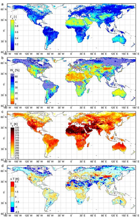
[38] First, Ts is calculated from the observed TB,37V
according to equation (2) (Figure 8c). Temperatures below
freezing are removed, as are grid cells with more than 4%
open water. Secondly, soil moisture data are used as derived
from TB,10 with the Land Parameter Retrieval Model
(LPRM) [Owe et al., 2008]. The LPRM soil moisture
retrieval does not yield moisture values when the vegetation
is too dense. These areas are masked in Figure 8b, and are
assigned a soil moisture of Wc = 25% in the simulation. This
Figure 7. As Figure 5, for frequency and incidence angle. arbitrary value does not affect the following discussion
because the dense vegetation effectively blocks the emission
from the soil. Third, the atmospheric transmissivity is
[35] Finally, open water will cause a negative bias in the parameterized according to Choudhury et al. [1992] using
retrieved temperature because the emissivity for water sur- precipitable water and cloud optical thickness data from the
faces is much lower then for land. Assuming that the water International Satellite Cloud Climatology Project (ISCCP
has the same temperature as the land surface, the bias can be [Rossow and Schiffer 1991]). The effective air temperature
estimated by calculating both open water and land surface is calculated as a direct function of surface temperature
brightness temperatures. Such analysis shows that for a [Bevis et al., 1992]. Because of this simplification, possible
vegetated land surface the bias as a function of the fraction errors due to asynchronous variations in the difference
of open water (F) is: (DT = 0.72F). This means that the bias between surface and air temperature are avoided. Finally,
will exceed 3 K if the fraction of open water in the satellite the vegetation transmissivity (Figure 8a) is parameterized
footprint exceeds 4%. Therefore 4% should be the maximum by means of the Microwave Polarization Difference Index
accepted fraction of open water when applying this method, (MPDI) according to Meesters et al. [2005]. The MPDI is
but preferably lower if a higher accuracy is required. calculated from the Ka band brightness temperatures:
[36] The conclusion of these simulations can be summa-
rized as follows. For vegetated surfaces, the effect of soil TB;V TB;H
MPDI ¼ ð3Þ
parameters is muted if the vegetation is dense (Gv 0.2). TB;V þ TB;H
The effect of soil moisture becomes important for less dense
vegetation, with errors of ±3 K at Gv = 0.35. The vegetation The atmospheric effect on this MPDI value is removed to
parameter single scattering albedo has the most effect on the obtain the top of vegetation MPDI.
error, and is calibrated at w = 0.06. This parameter is [39] These global maps of input data are subsequently
subsequently used as a global constant. At dry, almost bare used to simulate the TB,37V according to the radiative transfer
surfaces, the effect of soil parameters is very strong and that theory (see section 2.4). The difference between simulated
of vegetation parameters is of course very small. Soil and measured TB,37V is the error as introduced by the
moisture has an extreme effect in this scenario. The rough- simplification of the radiative transfer model to a single linear
ness parameter h and Q have a strong effect on the error too, relationship (equation (2)). The error in brightness tempera-
and are calibrated at h = 0.2 and Q = 0.2. These parameters ture is subsequently multiplied by the slope of the linear
are subsequently considered to be constant over time, and relationship to yield the corresponding error in Ts.
over the globe. [40] Figure 8d shows the global distribution of the bias in
the retrieved Ts, due to spatial variation in soil moisture, soil
3.3. Global Error Simulation texture, vegetation density and atmospheric vapor content.
[37] In actual applications of equation (2) on global Ka It can be seen that for large parts of the world this spatial
band observations, some of the above mentioned error variation in soil vegetation and atmospheric variables will
sources will cancel each other out. For example, vegetation not result in large errors in Ts. This is because, for 53% of
density and soil water content are, generally speaking, the globe, the transmissivity is less than 0.35 and for 72%
positively related. As was shown, the soil moisture values the Gv is less than 0.5. As was discussed above, areas where
that minimize the error are also positively related with Gv > 0.5 are expected to have a bias exceeding 3 K for at
vegetation density. This section explores the bias associated least part of the year. Areas with low vegetation and saturated
with the use of equation (2) as opposed to the radiative soil moisture conditions show a high negative bias (see for
transfer model, and as a result of the main spatially varying example Canada). This negative bias is increased if there is
parameters. For this purpose, the radiative transfer model is some open water in the pixel. Overall, for the land area with
applied to observed global input parameters and the resulting Gv < 0.5, 94% has a bias less than 3 K. This fraction decreases
modeled brightness temperatures are compared with equation to 87% for a bias ofD04113 HOLMES ET AL.: LAND SURFACE TEMPERATURE FROM KA BAND D04113
Figure 8. Main input and results of global error simulation. (a) Vegetation transmissivity at 37 GHz, (b)
soil moisture from LPRM-X with high vegetation densities masked (H), (c) land surface temperature (K),
and (d) bias ( uation (2), radiative transfer model)). The data are averaged for 1 and 2 July 2004.
9 of 15D04113 HOLMES ET AL.: LAND SURFACE TEMPERATURE FROM KA BAND D04113
Figure 9. Scatter diagram of the vegetation transmissivity against the bias (DT (K)), together with the
associated histograms for both variables. In red are the values with Wc < 15%, in black are values with
Wc > 35%, and green are intermediate moisture values.
content. The vertical line indicates the vegetation transmis- that the error associated with equation (2) is within accept-
sivity at which soil moisture becomes a critical factor in the able limits. Areas with unfavorable conditions have either
accuracy of the relationship for a 3 K limit. From Figure 9 (1) practically no vegetation or (2) sparse vegetation and
it can also be seen that for the pixels with low vegetation almost saturated soil moisture conditions.
density (Gv > 0.5) a large number of pixels is still within
acceptable limits. In these situations, the negative bias 3.4. Ground Validation
associated with the low vegetation density is offset by a [44] Equation (2) is validated by comparing temperature
positive bias, for example due to a very low soil moisture retrievals with ground observations of TLW from the
content. However, these same pixels are likely to fall outside FLUXNET stations described earlier. The procedure for
the limits for some of the year if the moisture conditions deriving TLW is outlined in section 2.2. Since equation (2)
change. is based on data from most of these sites in the first place, we
[42] In the above, the parameters for roughness (h, Q), and cannot validate the absolute accuracy of this method. How-
the single scattering albedo are treated as global constants. ever, it is possible to determine the precision of this method
Errors due to possible variations in these parameters are by looking at the standard error for each site individually.
evaluated in the Monte Carlo simulation for the same data [45] The comparisons of the satellite derived Ts and TLW
as described above. Global fields of roughness (h, Q) and derived for the field site are shown in Figure 11 and
single scattering albedo are not available and are attributed summarized in Figure 12. The field sites are separated into
random deviations from a given mean. The estimated stan- a group with low vegetation and one with high vegetation.
dard deviation associated with these parameters is listed in The low-vegetation group consists of the grassland, open
Table 2. In the Monte Carlo simulation this is repeated 500 shrubland and cropland sites. The high-vegetation group
times, so that the average of the deviations again approx- includes all the forest sites (see Table 1). For both groups,
imates the standard deviation for each parameter. Figure 10 correlations are high, with a median of R2 = 0.9 for the
shows the result of 500 iterations of the Monte Carlo low-vegetation group and R2 = 0.93 for the high-vegetation
simulation. The histograms show the distribution of the input group. The standard error of estimate (SEE) shows a clear
parameters. The standard error of the resulting temperature differentiation between the two groups. For forests, the SEE
relationship is 1.9 K. The average regression is indicated by is between 1.5 and 2.5 K, with a median of 2.2 K. The low
the solid black line, and the standard error bounds by the vegetation has SEE values between 2.3 and 4.5 K, with a
dashed lines. median of 3.5 K. A factor that might explain some of the
[43] The conclusion from these global simulations is that difference in performance between the low- and high-
for large parts of the E e surface conditions are such vegetation sites, is the seasonality in the longwave emissivity
10 of 15D04113 HOLMES ET AL.: LAND SURFACE TEMPERATURE FROM KA BAND D04113
Figure 10. Simulated TB,37V according to equation (2) for the globe.
as observed in the low-vegetation sites (see Figure 3). The error in the satellite temperature and should be avoided by
emissivity through the year at these sites is affected by the applying a strict mask for open water.
growing season of the vegetation. For this analysis, a constant [47] With this simple method to obtain Ts from TB,37V it is
e is used for the entire year. On the whole, these results possible to observe the diurnal temperature variation, using
indicate that Ts can be derived with a precision of 3.5 K for multiple satellites. This is shown in Figure 13 for the first 2
low vegetation and 2.2 K for forests. weeks of June 2006, for the forest site in North Carolina,
[46] Because of the inherent difficulties of comparing USA (site P). The satellites describe the diurnal cycle of
satellite data representing footprints of 25 25 km to single the ground measurements very well. Only at one instance,
point observations, it is difficult to use this analysis to further on 7 June, precipitation causes a serious negative error. After
constrain the accuracy as determined from the simulations. removing the observations that occur during rainfall, the
This is because the temperature at the ground site is not RMS error between satellite and ground observations is
necessarily a good representation for the satellite footprint. If 1.4 K, with a correlation of R2 = 0.94. Figure 14 shows a
the vegetation density at the ground site is low, but the second example for 2 weeks of June 2006, this time for
satellite footprint contains some forest, the temperature the grassland site in Montana, USA (site B). Again at one
cycles (diurnal and seasonal) will likely be more pronounced instance, on 6 June, precipitation causes a negative error.
at the field site. As a result, the slope of the regression will be Although the analysis of the full year of data showed this site
above unity (e.g., site A). The opposite will happen if the performing worse than the North Carolina site, this 2 week
ground site is located in a forest and the satellite footprint also period still shows a reasonably good RMS error between
contains less dense vegetation. This can result in a satellite and ground observations of 2.1 K, and a correlation
corresponding slope of below unity (e.g., site Q). The box of R2 = 0.90.
plot of the slope of the regression lines shows that both these
effects happen within the selected field sites (see Figure 12). 4. Discussion and Conclusion
The slope for the low-vegetation sites is between 1 and 1.37,
and for the high vegetation between 0.74 and 1.04. This [48] The Ka band vertical polarized passive microwave
means a large part of the variation in the slopes of the channel has a strong and linear relationship with the physical
observed regression lines can be explained by heterogeneity land surface temperature. It is shown that with a simple linear
in the satellite footprint and does not reflect an error in the relationship the Ts can be obtained for nonfrozen land
satellite temperature. Another example of a point-to-pixel surfaces and areas with little or no open water (D04113 HOLMES ET AL.: LAND SURFACE TEMPERATURE FROM KA BAND D04113
Figure 11. Satellite derived Ts is compared to ground measurements of TLW for 17 locations during
2005. The letters above each plot refer to the site IDs in Table 1.
12 of 15D04113 HOLMES ET AL.: LAND SURFACE TEMPERATURE FROM KA BAND D04113
Figure 12. Satellite derived Ts is compared to ground measurements of TLW for 17 locations during
2005. The box plots have horizontal lines between each data quartile of the selections for low vegetation
(low) and high vegetation (high). Outliers are indicated with pluses.
original observed signal. The satellite observed Ts represents precision of the retrieved land surface temperature. If this
the area weighted average of the different land covers in the method is applied to all available vertically polarized 37 GHz
sensors view and can therefore best be compared to the observations, a 30 year record of land surface temperature
longwave temperature and not with a soil or vegetation can be obtained. For much of this period this set would
temperature at a fixed depth. A comparison of the retrieved include several observations per day. Complicating the
temperature with ground observations of longwave temper- interpretation of such a long-term data set would be the
ature yielded a SEE of 3.5 K for low vegetation and 2.5 different overpass times for each satellite and possibly
for forest, individually for each site. These errors result orbital decay over a satellites lifetime.
from (1) the precision of the microwave sensor (0.6 K for [49] For periods with multiple observations per day it is
AMSR-E), (2) a temporal change in the bias as introduced shown that the diurnal temperature cycle can be approxi-
by the model and nonstatic surface characteristics, (3) a mated from remote sensing data with a surprisingly high
temporal change in heterogeneity effects of the site versus precision. Because the partitioning of the surface energy
the pixel, and (4) precision and accuracy of the longwave balance is strongly related to surface temperature, the ampli-
measurements. The last two points are purely caused by the tude of the diurnal temperature variation can be of value for
validation method, and do not reflect an actual error with studies of latent and sensible heat fluxes at a global scale.
the area averaged temperature. For this reason, the SEE Since such studies make use of temperature differences, the
values are expected to represent an upper limit for the possible bias in the observations is less of a problem.
Figure 13. Diurnal temperature cycles as measured at a field site in North Carolina, USA, and observed
by satellites.
13 of 15D04113 HOLMES ET AL.: LAND SURFACE TEMPERATURE FROM KA BAND D04113
Figure 14. Diurnal temperature cycles as measured at a field site in Montana, USA, and observed by
satellites.
However, further research will be necessary to widen the Colwell, R., D. Simonett, and F. Ulaby (Eds.) (1983), Manual of Remote
Sensing, vol. 2, Interpretation and Applications, 2nd ed., Am. Soc. of
scope of this approach in sparsely vegetated areas. Photogramm., Falls Church, Va.
David, T. S., M. I. Ferreira, S. Cohen, J. Pereira, and J. David (2004),
[50] Acknowledgments. This work was partly funded by the EU 6th Constraints on transpiration from an evergreen oak tree in southern
Framework program WATCH (project 036946-2). We appreciate the help Portugal, Agric. For. Meteorol., 122, 193 – 205.
from Michiel van der Molen with the longwave emissivity derivation and DeAngelis, R., P. Valentini, G. Matteucci, R. Monaco, S. Dore, and G. E. S.
the helpful comments of John Gash. We thank the organizations who Mugnozza (1996), Seasonal net carbon dioxide exchange of a beech
support the FLUXNET sites (Illinois State Water Survey, INRA, Max Planck forest with the atmosphere, Global Change Biol., 2(3), 199 – 207.
Institute Jena, NOAA/ARL, Universidade Técnica de Lisboa, University of De Jeu, R. A. M., and M. Owe (2003), Further validation of a new metho-
Tuscia Viterbo, Wageningen University, and Weisman Institute of Science) dology for surface moisture and vegetation optical depth retrieval, Int.
for making the data available to us. J. Remote Sens., 24(22), 4559 – 4578.
Dolman, A., E. Moors, and J. Elbers (2002), The carbon uptake of a mid
latitude pine forest growing on sandy soil, Agric. For. Meteorol., 111(3),
References 157 – 170.
Anthoni, P. M., A. Knohl, C. Rebmann, A. Freibauer, M. Mund, W. Ziegler, Fily, M., A. Royer, K. Goı̈ta, and C. Prigent (2003), A simple retrieval
O. Kolle, and E. Schulze (2004), Forest and agricultural land-use- method for land surface temperature and fraction of water surface deter-
dependent CO2 exchange in Thuringia, Germany, Global Change Biol., mination from satellite microwave brightness temperatures in sub-arctic
10(12), 2005 – 2019. areas, Remote Sens. Environ., 85, 328 – 338.
Armstrong, R., K. Knowles, M. Brodzik, and M. Hardman (1994), DMSP Grunzweig, J. M., T. Lin, E. Rotenberg, A. Schwartz, and D. Yakir (2003),
SSM/I pathfinder daily EASEGrid brightness temperatures, http:// Carbon sequestration in arid-land forest, Global Change Biol., 9(5),
www.nsidc.org/data/nsidc-0032.html, Natl. Snow and Ice Data Cent., 791 – 799.
Boulder, Colo. Hollinger, S., C. Bernacchi, and T. Meyers (2005), Carbon budget of mature
Ashcroft, P., and F. Wentz (2003), AMSR-E/AQUA L2A global swath no-till ecosystem in north central region of the united states, Agric. For.
spatially-resampled brightness temperatures (Tb) v001, http://www. Meteorol., 130, 59 – 69.
nsidc.org/data/ae_l2a.html, Natl. Snow and Ice Data Cent., Boulder, Colo., Kerr, Y. H., P. Waldteufel, J.-P. Wigneron, J.-M. Martinuzzi, J. Font, and
(Updated daily.) M. Berger (2001), Soil moisture retrieval from space: The Soil Moisture
Baldocchi, D., et al. (2001), FLUXNET: A new tool to study the temporal and Ocean Salinity (SMOS) mission, IEEE Trans. Geosci. Remote Sens.,
and spatial variability of ecosystem-scale carbon dioxide, water vapor, and 39(8), 1729 – 1735.
energy flux densities, Bull. Am. Meteorol. Soc., 82, 2415 – 2434. Kowalski, S., M. Sartore, R. Burlett, P. Berbigier, and D. Loustau (2003),
Beljaars, A., and F. Bosveld (1997), Cabauw data for the validation of land The annual carbon budget of a French pine forest (pinus pinaster) follow-
surface parameterization schemes, J. Clim., 10(6), 1172 – 1193. ing harvest, Global Change Biol., 9(7), 1051 – 1065.
Belward, A. S., J. E. Estes, and K. D. Kline (1999), The IGBP-DIS global Kummerow, C., W. Barnes, T. Kozu, J. Shiue, and J. Simpson (1998), The
1-km land-cover data set DISCover: A project overview, Photogramm. Tropical Rainfall Measuring Mission (TRMM) sensor package, J. Atmos.
Eng. Remote Sens., 65, 1013 – 1020. Oceanic Technol., 15, 809 – 817.
Bevis, M., S. Businger, T. Herring, C. Rocken, R. Anthes, and R. Ware Meesters, A. G. C. A., R. A. M. De Jeu, and M. Owe (2005), Analytical
(1992), GPS meteorology—Remote-sensing of atmospheric water-vapor derivation of the vegetation optical depth from the Microwave Polariza-
using the global positioning system, J. Geophys. Res., 97, 15,787 – 15,801. tion Difference Index, IEEE Geosci. Remote Sens. Lett., 2(2), 121 – 123,
Calvet, J., J. Wigneron, A. Chanzy, S. Raju, and L. Laguerre (1995), Micro- doi:10.1109/LGRS.2005.843983.
wave dielectric properties of a silt-loam at high frequencies, IEEE Trans. Mo, T., B. J. Choudhury, and T. Jackson (1982), A model for microwave
Geosci. Remote Sens., 33, 634 – 642. emission from vegetation-covered fields, J. Hydrol., 184, 101 – 129.
Choudhury, B. J., E. R. Major, E. Smith, and F. Becker (1992), Atmospheric Njoku, E., T. Jackson, V. Lakshmi, T. Chan, and S. Nghiem (2003), Soil
effects on SMMR and SSM/I 37 GHz polarization difference over the moisture retrieval from AMSR-E, IEEE Trans. Geosci. Remote Sens., 41,
Sahel, Int. J. Remote Sens., 3443 – 3463. 215 – 229.
14 of 15D04113 HOLMES ET AL.: LAND SURFACE TEMPERATURE FROM KA BAND D04113
Owe, M., and A. Van de Griend (2001), On the relationship between Ulaby, F. T., R. K. Moore, and A. K. Fung (1986), Microwave Remote
thermodynamic surface temperature and high-frequency (37 GHz) verti- Sensing: Active and Passive, vol. III, From Theory to Applications,
cally polarized brightness temperature under semiarid conditions, Int. Artech House, Norwood, Mass.
J. Remote Sens., 22, 3521 – 3532. Van de Griend, A. A., and M. Owe (1994), Microwave vegetation optical
Owe, M., R. A. M. De Jeu, and J. P. Walker (2001), A methodology for depth and signal scattering albedo from large scale soil moisture and
surface soil moisture and vegetation optical depth retrieval using the NIMBUS/SMMR satellite observatons, Meteorol. Atmos. Phys., 54,
microwave polarization difference index, IEEE Trans. Geosci. Remote 225 – 239.
Sens., 39(8), 1643 – 1654. Verstraeten, W., F. Veroustraete, C. Van der Sande, I. Grootaers, and J. Feyen
Owe, M., R. De Jeu, and T. Holmes (2008), Multi-sensor historical clima- (2006), Soil moisture retrieval using thermal inertia, determined with visi-
tology of satellite derived global land surface moisture, J. Geophys. Res., ble and thermal spaceborne data, validated for European forests, Remote
113, F01002, doi:10.1029/2007JF000769. Sens. Environt., 101, 299 – 314.
Pampaloni, P., and S. Paloscia (1986), Microwave emission and plant water Wang, J. R., and B. J. Choudhury (1981), Remote sensing of soil moisture
content: A comparison between field measurements and theory, IEEE content over bare field at 1.4 GHz frequency, J. Geophys. Res., 86(C6),
Trans. Geosci. Remote Sens., 24, 900 – 905. 5277 – 5287.
Penman, H. L. (1948), Natural evaporation from open water, bare soil and Wang, J. R., and T. J. Schmugge (1980), An empirical model for the
grass, Proc. R. Soc. London, Ser. A, 193, 120 – 145. complex dielectric permittivity of soils as a function of water content,
Rossow, W., and R. Schiffer (1991), ISCCP cloud data products, Bull. Am. IEEE Trans. Geosci. Remote Sens., 18(4), 288 – 295.
Meteorol. Soc., 71, 2 – 20.
Rossow, W., A. Walker, and L. Gardner (1993), Comparison of ISCCP and
other cloud amounts, J. Clim., 6, 2396 – 2416. R. A. M. De Jeu, A. J. Dolman, and T. R. H. Holmes, Department of
Scherer-Lorenzen, M., E. Schulze, A. Don, J. Schumacher, and E. Weller Hydrology and Geo-Environmental Sciences, Vrije Universiteit, NL-1081
(2007), Exploring the functional significance of forest diversity: A new HV Amsterdam, Netherlands. (thomas.holmes@falw.vu.nl)
long-term experiment with temperate tree species (BIOTREE), Perspect. M. Owe, Hydrological Sciences Branch, NASA Goddard Space Flight
Plant Ecol. Evol. Syst., 9, 53 – 70, doi:10.1016/j.ppees/2007.08.002. Center, Greenbelt, MD 20771, USA.
Snyder, W. (1999), Classification-based emissivity for land surface tempera-
ture measurement from space, Int. J. Remote Sens., 19, 2753 – 2774.
15 of 15You can also read