Lawrence Berkeley National Laboratory - Recent Work
←
→
Page content transcription
If your browser does not render page correctly, please read the page content below
Lawrence Berkeley National Laboratory
Recent Work

Title
81-beam coherent combination using a programmable array generator.

Permalink
https://escholarship.org/uc/item/6n799961

Journal
Optics express, 29(4)

ISSN
1094-4087

Authors
Du, Qiang
Wang, Dan
Zhou, Tong
et al.

Publication Date
2021-02-01

DOI
10.1364/oe.416499

Peer reviewed

 eScholarship.org                              Powered by the California Digital Library
                                                               University of California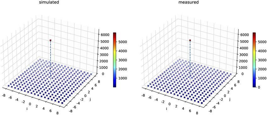
Research Article                                    Vol. 29, No. 4 / 15 February 2021 / Optics Express   5407

81-beam coherent combination using a
programmable array generator
Q IANG D U , *           DAN WANG , T ONG Z HOU , D ERUN L I ,                         AND      R USSELL
W ILCOX
Lawrence Berkeley National Lab, 1 Cyclotron Road, Berkeley, CA 94720, USA
* QDu@lbl.gov

Abstract: We have generated 81 independently controllable beams using a spatial light modulator
and combined them on a diffractive combiner, to characterize the combiner and develop a fast
phase error detection scheme. A key parameter of the diffractive combiner is measured in a
new way, enabling an efficient combination when programming calibrated phases of each beam.
This testbed provides a platform for development of advanced feedback phase control of high
channel-count beam combination.

© 2021 Optical Society of America under the terms of the OSA Open Access Publishing Agreement

1.   Introduction
Recent reports have emphasized the importance of high energy, high repetition rate ultrafast
lasers for scientific applications [1]. We have been developing fiber technology to meet this
need, with the goal of driving laser plasma accelerators [2]. Recent work in large mode area,
temporally combined fiber lasers has demonstrated ∼ 10mJ per amplifier output [3]. To reach
multi-Joule-level pulse energies needed for our application, 100s of outputs will have to be
spatially combined, making it important to minimize the number of combining optics. Currently,
ultrafast, high power pulse combination uses binary trees of 2-way combiners, or splitter arrays
[4]. High channel-count, tiled-aperture coherent combining has been reported [5] with ∼ 50%
efficiency, however close-packed tiled aperture combining has an intrinsic 67% theoretical limit.
High average power CW combination can be done using a single diffractive optical element
(DOE) [6], but this scheme incurs efficiency-limiting angular dispersion if broadband pulses are
used.
   We recently demonstrated a two-diffractive-element scheme which compensates or minimizes
dispersions, combining eight 120fs pulses with no pulse distortion [7–9]. We also stabilized
combining efficiency against perturbations using a new algorithm based on pattern recognition,
sensing the uncombined beam intensities on a camera as data [10]. To show how this stabilization
algorithm scales to realistic numbers of beams it would be possible to simply expand the 8-beam
experiment by assembling a large array of phase shifters, collimators and mirrors, but this would
be cumbersome and expensive. Instead, we chose to generate a controllable beam array more
simply and input this into a larger channel-number diffractive splitter, creating a convenient
platform for algorithm development.
   We chose a commercial off-the-shelf diffractive splitter instead of designing our own DOE, to
show that this characterization and control method is generic, not specific to a specially designed
combining element, and is suitable for any diffractive coherent beam combining analysis. In
the case of a specially designed DOE, this measurement method can be a way of experimental
verification against fabrication errors.
   For coherent beam combining, a widely used method of phase error measurement is interfer-
ometric technique [5,11], which uses an expanded reference beam to generate interferograms
for each channel. The phase error measurement accuracy is limited by the number of pixels per
fringe and camera dynamic range. In comparison, our method does not require a reference beam,

#416499                                                                      https://doi.org/10.1364/OE.416499
Journal © 2021           Received 7 Dec 2020; revised 26 Jan 2021; accepted 27 Jan 2021; published 4 Feb 2021
Research Article                              Vol. 29, No. 4 / 15 February 2021 / Optics Express   5408

is not subject to fringe limitation, the characterization only needs to be done using one optical
element (Spatial Light Modulator, SLM), and is fully programmable and reproducible. The
physical model built upon this method could be then used for feedback algorithm developments.

2.      Beam array formation using a spatial light modulator
Having previously shown that the diffractive optic pair works with short pulses, we used a CW
signal instead, with no change to the combining principle. 81 beams were formed and controlled
using a spatial light modulator (Hamamatsu X13138–02) as shown in Fig. 1.

          Fig. 1. SLM combiner experiment. DOE: diffractive optical element. FF: beam intensity
          flattening filter.

   A CW source produces a beam which is collimated, flattened using a Gaussian ND filter, then
sent to the SLM at near normal incidence. The SLM is a programmable phase hologram (in
this case, a set of blazed gratings diffracting light into the first order), enabling control over all
beam parameters except polarization; location, size, intensity profile, two directions of angle,
amplitude and phase, as listed in Table 1. It is possible to move the grating lines parallel to their
spacing in sub-period increments, which varies the phase of the diffracted beam dynamically,
enabling control of each beam. The CW beam at 1030 nm illuminates the entire SLM area of
1272 × 1024 pixels, where smaller zones diffract light to produce 81 independent beams, which
converge on the 9 × 9 diffractive splitter (MS-259 from Holo/Or). The resultant 2D fan of beams
is captured by a lens and a camera (Teledyne Dalsa Genie Nano M1280 NIR). The camera has an
OnSemi Python1300 P1 (1.3M) sensor without gamma corrections, and the response is linear
with respect to the number of photons received by the sensor. Camera is configured with Mono
10-bit pixel format readout through Ethernet at 30 frames per second, at a fixed exposure time
without analog gain (39.7 dB SNR), so the sensor sensitivity is constant. In this way, we can
form a 9 × 9 array of independently controlled beams without difficulty.

            Table 1. Each beam has independent control of parameters in beam array formation
Beam Parameter                                                                        Hologram control
 Tilt Angle in x                                                              Modulation spatial frequency in x
 Tilt Angle in y                                                              Modulation spatial frequency in y
     Position in x                                                                  Centroid location in x
     Position in y                                                                  Centroid location in y
Transverse Profile                                                                Modulation depth function
     Amplitude                                                                  Modulation depth mean value
        Phase                                                                         Modulation offset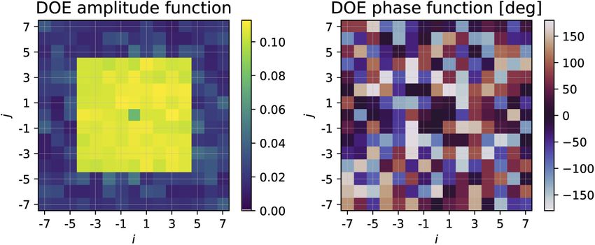
Research Article                               Vol. 29, No. 4 / 15 February 2021 / Optics Express   5409

   The generation of an input beam array can be updated at up to 60 Hz. The parameters are
calculated using the inverse 2D Fourier transform and experimentally optimized to form a cone
of beams converging at the DOE plane. We choose a circular flat-top transverse beam profile for
best diffraction efficiency and beam separation, versus a square or Gaussian profile.
   Figure 2 is an example of the generated hologram for 81 converging beams with balanced
amplitudes, compensating uneven input beam power caused by variations in SLM efficiency as a
function of horizontal diffraction angle.

       Fig. 2. Hologram on SLM for generating 9 × 9 beams. Gray level corresponds to grating
       modulation depth.

   At the output, a camera images the beam pattern emerging from the DOE. For N × N input
beams and a N × N shaped d(i, j), there will be (2N − 1) × (2N − 1) outputs, because each input
beam produces 9 × 9 outputs, always overlapped at the center beam. The beam size on the camera
is of approximately 22 pixels in diameter.
   Since the beams are formed by diffraction from programmed phase gratings, there must be
enough pixels per grating line, and enough lines per beam, to achieve adequate diffraction
efficiency. Also, as the number of pixels per line pair diminishes, aliasing in the digital image
produces spurious higher order beams which can interfere with the wanted beams. The SLM
pixel pitch is 12.5 µm, and the smallest width is 12.8 mm. We want a square array of 9×9 beams,
so each diffracting spot will be smaller than 12.8/9 = 1.4 mm diameter. Geometry of the optical
setup limits the minimum diffraction angle to about 17 mrad, but, depending on beam position,
there will be an additional angle of up to 16.2 mrad to allow for the required convergence into
the diffractive splitter (designed as 16.7 mrad at 1064 nm but operated here at 1030 nm). So,
diffraction angles are between 17 and 33 mrad, requiring from 16 lines/mm to 32 lines/mm
respectively. This provides for only 2.5 pixels per line at the higher density, which is marginal.
Diffraction efficiency for the high angle side of the SLM is low, but adequate for this experiment.

3.   Analysis of DOE transmission function measurement
In order to achieve efficient beam combination, the splitter DOE must be presented with an input
beam array with the correct phases (the same phases produced when the DOE splits one beam
into many). Here is how to experimentally get them by DOE characterization.
Research Article Vol. 29, No. 4 / 15 February 2021 / Optics Express 5410
Consider a 2D DOE grating with a intrinsic complex transmittance
t(x, y) = |t(x, y)|ej∠t(x,y)
where |t(x, y)| and ∠t(x, y) are the amplitude and phase of the transmittance. Designed as a
diffraction splitter, t(x, y) is only non zero at certain diffraction orders, so we can express t(x, y)
as a discrete complex function d(i, j), where i, j are integers, representing the order number in x
and y axes respectively.
Then the physical process of 2D diffractive combining is known [10,12] as a 2D convolution
of the discrete complex input beam function b(i, j) with d(i, j)
∞
∑︂ ∞
∑︂
s(i, j) = b(i, j)d(i − m, j − n)
m=−∞ n=−∞ (1)
= b(i, j) ∗ ∗d(i, j)
where
i, j, m, n ∈ Z, s(i, j), b(i, j), d(i, j) ∈ C2
The resulting s(i, j) is the complex amplitude of diffracted beam at far field; and (i, j) is the
integer Cartesian coordinate of either input beam array or far field diffracted beam array from the
incident direction, centered at the center input beam or zero order diffracted beam at (0, 0). For
the following discussion, the absolute phase modulation on the zero order beam, ∠d(0, 0) = 0, is
ignored because only the relative phases between the diffracted beams are of interest for coherent
combining.
We measure d(i, j) in order to understand which output patterns correspond to which input
phases, and to derive phase errors from output patterns. The phase of d(i, j), as ∠d(i, j), is
typically not intentionally designed, but is the result of an automated genetic algorithm search for
the highest efficiency DOE design, with phases as free parameters [13]. ∠d(i, j) is a characteristic
of the combining element, and can be found experimentally by correlating the intensities of
output spots contributed to by only two input beams with the relative phase between those input
beams. With that information, we can predict the output pattern given any set of amplitudes and
phases of the inputs.
When the measurements of d(i, j) are complete, we have the intrinsic phase function and can
predict output patterns given any arbitrary input, as well as present the DOE with an ideally
phased beam array. Optimal combining requires that all incident beams constructively add to the
zeroth order diffracted beam, a phase condition which can be defined as
∠b(i, j) = −∠d(−i, −j) (2)
which means that the DOE is presented with a beam array which matches its intrinsic phase
function. When this input array is other than ideal, there will be excess loss.
The coherent combining efficiency loss as a function of equal probability, uncorrelated RMS
piston phase error σφ (in radian) from each channel is 1 − η = σφ2 . [14] This is the main
contribution to error we observe in practice, and the main subject of our control efforts. To
achieveResearch Article Vol. 29, No. 4 / 15 February 2021 / Optics Express 5411
to the phases by
|s(i, j)| 2 = 2 + 2 cos (∆ϕ + ∆θ) (3)
where ∆ϕ is the relative input beam phase, and ∆x θ, ∆y θ is the difference function of the intrinsic
phase in each direction:
{︄
∆x θ(i, j) = θ(i, j) − θ(i − 1, j) Horizontal
∆θ =
∆y θ(i, j) = θ(i, j) − θ(i, j − 1) Vertical
In practice, we can easily know the rate of phase scanning by knowing how the SLM grating
lines move across the beams, but the additional phase offset (which we want to find) needs to be
measured against a fixed “zero” or else there is an additional arbitrary additive term. We choose
this point by adjusting the phases of the reference beam and the test beams relative to the center
beam, to maximize their contributions to center beam power, establishing a “zero” relevant to
the optimal combining condition according to Eq. (2). Then, we scan the reference beam over
several cycles (varying ∆ϕ), and record the sinusoidal power variations of each output beam.
Fourier analysis of these power variations gives the phase scanning frequency ω0 and an offset
phase function Φ(i, j) for each case:
∂∠|s(i, j)|
= ω0 , ∆θ(i, j) + ∆ϕ0 = Φ(i, j)
∂∆ϕ
where ∆ϕ0 = −∆θ(−ir , −jr ) is the initial relative input beam phase for each case, which is part of
the “zero” condition, so that the derived θ(i, j) is independent of the selection of reference beam.
This gives the difference function of the DOE phase function ∆x θ, ∆y θ, which can be
cumulatively summed across the range of beam positions to yield the estimated intrinsic DOE
phase function θ̂(i, j).
(︄ )︄
∑︂ ∑︂
θ̂ x (i, j) = ∆x θ(i, j) + ∆y θ(i, 0)
−B≤i≤B −B≤i≤B
(︄ )︄
∑︂ ∑︂
θ̂ y (i, j) = ∆y θ(i, j) + ∆x θ(0, j)
−B≤j ≤B −B≤j ≤B
{︄
N−1
1 (︂ )︂ if N is odd
θ(i,ˆ j) = θ̂ x (i, j) + θ̂ y (i, j) , B= N
2
2 2 if N is even
Here the starting row or column for summation can be arbitrary; we choose to start from the
center and sum in both directions, so that an unlimited number of higher order beams could be
included. Averaging θ̂ x (i, j), θ̂ y (i, j), and possibly from more symmetric cases would improve
measurement accuracy.
4. Experimental measurement of a DOE transmission function
The reference beam is not necessarily be the center, 0th order beam because, for our arrangement,
the SLM grating lines are exactly vertical, aligned with the SLM pixels in the center row
(horizontal diffraction only). The effects of aliasing, given the marginal resolution in this case,
are severe for those spots. Other rows where the lines slant (vertical and horizontal diffraction
together), cutting across columns of pixels, tend to average out the effects of aliasing and give
much cleaner data.
This derivation from measurement is directly analogous to the simpler case of two beam
combination where an intrinsic phase offset needs to be found, if, for instance, feedbackResearch Article Vol. 29, No. 4 / 15 February 2021 / Optics Express 5412
stabilization was based on output intensity. The difference here is that we are dealing with a large
matrix of beams all at once, as in Eq. (3).
For example, when only two beams at (0, 1) and (0, 2) are enabled, and the phase of one
beam is scanned, the resulting changing interference pattern is a function of the intrinsic DOE
phase difference function ∆θ and the phase difference offset of these two beams ∆ϕ. The phase
estimation from measured sinusoidal response of the diffraction pattern function |s(i, j)| 2 is the
summation of them, as shown in Fig. 3.
Fig. 3. Diffracted beam power is a function of DOE modulated beam phase, as illustrated
by two-beam interference analysisResearch Article Vol. 29, No. 4 / 15 February 2021 / Optics Express 5413
For this and all subsequent processed camera images, the axes are indices i and j, with each
small square a color-mapped value of the integrated power within it. The units of plots are
indicated in each caption.
Selecting input beam (ir , jr ) = (0, 1) as a reference, the vertical and horizontal DOE transmission
difference phase function can be measured by analyzing interference pattern of test beam (0, 2)
and (−1, 1) respectively, when scanning the phase of reference beam (0, 1). The results are
recorded as two videos of interference patterns, indexed by reference beam scanning phase.
Because the phase scanning speed ω0 is constant and common to all cases, a Fourier analysis at
this frequency gives both magnitude and phase function Φ(i, j) for either horizontal or vertical
test cases.
From its magnitude response as shown in Fig. 3(c), unwanted frequency components from
noise and aliasing effects are filtered out, so only the phase response on the known scanning
frequency ω0 is extracted. The “zero” condition is found by tuning the test beam phase and
maximizing the center combined beam |s(0, 0)| 2 .
For both horizontal and vertical test cases, we found that using the opposite side test beam, i.e.,
(0, 0) and (1, 1) respectively, gives a negative phase function −Φ(i, j) of each phase with great
accuracy, as shown in Fig. 4.
Fig. 4. Differences of Φ measured between opposite test beams. RMS estimation error is
less than 1.6◦ . Color bar unit is degree.
We also take advantage of this over-complete set of measurements for averaging, to achieve
better precision of the final DOE phase function estimation. The measured difference functions
of the DOE phase function in each direction are shown in Fig. 5.
After cumulative summation in both directions, the final DOE phase function θ(i, j) is derived.
A plot of the calculated d(i, j) is shown in Fig. 6. The amplitude function is from a power
distribution measured with only the center input beam with total power normalized to 1, so that
each first√︁ order diffracted beam amplitude is approximately the DOE amplitude splitting fraction
Dn = 1/81 = 1/9. The measured phase function hasResearch Article Vol. 29, No. 4 / 15 February 2021 / Optics Express 5414
Fig. 5. Measured DOE difference phase functions in both directions. Color bar unit in
phase plot is degree. Only overlapped locations in diffractive pattern are shown, resulting in
9 × 8 and 8 × 9 shape for horizontal and vertical test cases respectively.
Fig. 6. Measured d(i, j) of size 15 × 15 for a 9 × 9 DOE. Amplitude function is a unit-less
amplitude transmission efficiency, and phase function unit is degree. The overall DOE power
transmission efficiency is normalized to a lossless 100% despite uniformity.
5. Experimental combining of 81 beams
After d(i, j) is characterized, it can be used to measure the actual input beam phase with respect
to its SLM hologram phase shifting parameter. With the center input beam fixed as a reference,
each input beam is introduced and its phase is scanned by shifting the SLM grating lines with
sub-pixel resolution, so that the resulting two-beam interference pattern as a function of difference
phase can be recorded. Both amplitude balancing and phase calibration can be achieved by this
automated process for each input beam. As shown in Fig. 2, for a desired uniform-power inputResearch Article Vol. 29, No. 4 / 15 February 2021 / Optics Express 5415
beam array, the beam amplitude or SLM modulation depth is a function of SLM diffraction
efficiency which is inversely proportional to spatial frequency (or diffraction angle), plus laser
source power distribution. The input beam phase is a linear function of SLM grating line
displacement, with a coefficient proportional to diffraction angle. After calibration, when the
ideal beam phases described in Eq. (2) are programmed into the SLM, the coherent combination
of 81 beams is achieved, resulting in a powerful center combined beam surrounded by low
amplitude uncombined beams.
In order to compare the simulated and measured diffraction pattern, a linear calibration of
beam power to camera sensitivity is required. We did this by introducing one input beam at a
time, while measuring the combined center beam power. We found that the combined beam
power is quadratic with the number of input beams as shown in Fig. 7, meaning that the power is
moving from side beams to the center when adding more beams, which is what is intended.
Fig. 7. Measured combined beam power when adding one beam at a time, as calibration
between camera reading and simulation. Additive combined power is proportional to number
of beams before the camera starts to saturate starting at 13th input beam, confirming the
quadratic power increase. The quadratic polynomial fit matches well with simulated data
using ideal beams after linear calibration.
In this work, we are using the camera more like a power meter, which responds to the
area-integrated photocurrent irrespective of the beam size incident on the sensor. We do the
same thing by integrating over an area, that covers the diffracted beam size. The power is in our
special units, not the usual Watts, because we are concerned with ratios of power, not absolute
measurements. We define one power unit as the power of one diffracted spot after the DOE,
when one beam is incident. This will be 1/81 of the incident beam power. When the 81 beams
are optimally combined, the output power in the central beam will be 81 times the power of
one input beam, and 812 times the power of our defined power unit. Our simulation captures
the measured 5% uniformity of DOE splitting efficiency, and the 55% zero-order relative to the
average, without impacting the above theoretical expectations.
The power contrast between the combined beam and the side beams increases when more beams
are added, and will easily go beyond the camera’s dynamic range, resulting in an incomplete
measurement due to camera saturation. The data from unsaturated camera measurement is still
able to provide enough information for phase corrections, as shown in a machine learning based
pattern recognition method [15], where the controller only cares about the side beams’ power.
The required signal-to-noise ratio (SNR) of the camera, limited by the brightest side beam in theResearch Article Vol. 29, No. 4 / 15 February 2021 / Optics Express 5416
diffraction pattern, is 29.7 dB, which is the ratio between the brightest side beam power and the
lower limit of 10% of a beam power unit. We have shown that a camera noise of RMS 10% of
the power unit is acceptable for the feedback to be stable [15]. Such SNR is achievable using a
typical 10-bit or 12-bit pixel format camera.
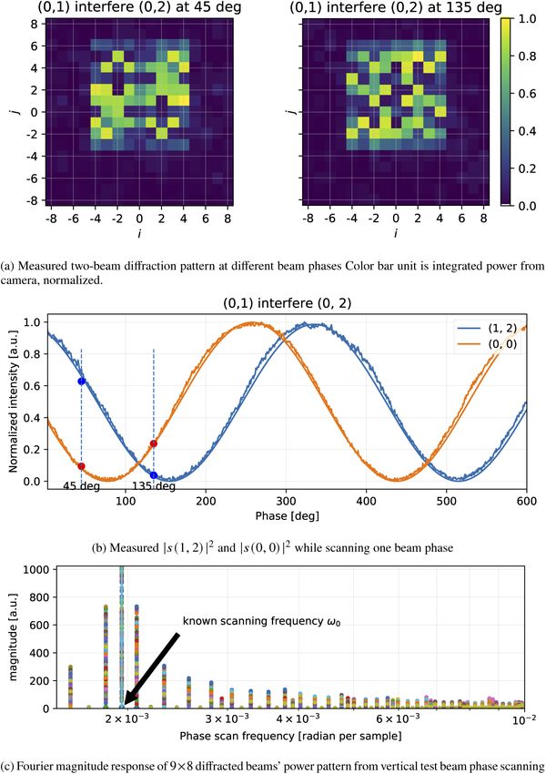
We calculate an array of such integrated values on the grid, as the raw readings of the diffraction
pattern, and calibrate it against theoretical values using the method described above, resulting the
measured diffraction pattern |s(x, y)| 2 , which is compared with simulation as shown in Fig. 8.
The RMS noise from the 10-bit camera is ∼ 0.15 in the same units.
Fig. 8. Calculated and measured beam patterns for optimized 81 beam combination. Color
bar unit is 1/81 of one input beam’s power.
The difference between the measured and simulated patterns results from imperfect beam
alignment, amplitude balancing, calibration error and noise. A difference of 8.4 RMS indicates
that the derived DOE intrinsic transmittance function is accurate enough to provide a basis for
further development of feedback stabilization of the combining process, as shown in Fig. 9. We
found that this RMS power difference based on the 15 × 15 model is improved by 1.5 compared
with the 9 × 9 (first order only) simulation result, confirming the value of including higher order
beams in determining d(i, j).
Fig. 9. Statistics of difference between simulated and measured diffraction pattern after
combining 81 beams. Color bar unit is 1/81 of one input beam power.
We want to emphasize that the 2D complex transmittance function d(i, j) is a complete
description of the diffractive combining process, as explained in the wave superposition equationsResearch Article Vol. 29, No. 4 / 15 February 2021 / Optics Express 5417
in Leger’s paper [12]. This intrinsic function is independent of experimental conditions such as
overall incident beam angles and positions on the DOE. We demonstrated this when we built
another test setup with different overall beam angle, beam size and position, and we found the
coherent combining process is reproducible; 81 beams could be combined using the same d(i, j)
and combining phase condition of Eq. 2.
Figure 10 shows the full-scale simulated and measured diffraction patterns when 81 beams
are combined in the new test setup. The contrast between the combined beam and the brightest
side beam at (4, −5) is 18.1 dB in simulation and 19.9 dB in measured data respectively. The
better-than-simulation contrast may be explained by higher order beams not included in the
model, similar to the previous result shown in Fig. 9. Defined as the ratio of combined center
beam power to total diffracted beam power, the combining efficiency measured is 60.4%, which is
reasonable compared with simulated combining efficiency of 65.3%, and given the DOE splitting
efficiency (DOE-limited maximum combining efficiency) of 72%. The modeled efficiency may
be less than the theoretical maximum due to our not including all the higher order diffracted
beams, and other errors in measurement. We made no attempt to optimize efficiency, but will
pursue this in future work.
Fig. 10. Simulated diffraction pattern and raw camera image when combined. Measured
data is from multiple expsure camera images to avoid saturation. Color bar unit on both
plots is 1/81 of one input beam power.
6. Conclusion
In conclusion, we have demonstrated a new way to generate a large beam array for coherent
combination research, used it to characterize a diffractive element in detail, and experimentally
combined 81 beams with high fidelity. This provides the basis for the phase detection scheme we
are investigating using side beam pattern recognition. This demonstration shows the similarity of
the coherent combining physical model to the measured result, and establishes the theoretical
foundation and experimental testbed for pattern based feedback control algorithm development,
including recently reported machine-learning based control [15–17]. These results are a significant
step toward kHz, ultrafast pulsed laser beam combination with an arbitrarily large number of
beams, for scaling to high energy.
Funding. Office of Science (DEAC02–05CH11231).
Acknowledgments. This work was supported by the Early Career Research Program of U.S. Department of Energy,
and the Laboratory Directed Research and Development Program of Lawrence Berkeley National Laboratory, under U.S.
Department of Energy Contract No. DE-AC02–05CH11231.
Disclosures. The authors declare no conflicts of interest.Research Article Vol. 29, No. 4 / 15 February 2021 / Optics Express 5418
References
1. R. Falcone, F. Albert, F. Beg, S. Glenzer, T. Ditmire, T. Spinka, and J. Zuegel, “Workshop report: Brightest light
initiative,” Tech. rep., OSA Headquarters, Washington, D.C, United States (2019).
2. W. Leemans, “Workshop report: Laser technology for k-bella and beyond,” Tech. rep., Lawrence Berkeley National
Laboratory (2017).
3. H. Pei, J. Ruppe, S. Chen, M. Sheikhsofla, J. Nees, Y. Yang, R. Wilcox, W. Leemans, and A. Galvanauskas, “10mJ
energy extraction from Yb-doped 85µm core CCC fiber using coherent pulse stacking amplification of fs pulses,” in
Advanced Solid State Lasers, (2017), pp. AW4A–4.
4. M. Müller, C. Aleshire, A. Klenke, E. Haddad, F. Légaré, A. Tünnermann, and J. Limpert, “10.4 kw coherently
combined ultrafast fiber laser,” Opt. Lett. 45(11), 3083–3086 (2020).
5. I. Fsaifes, L. Daniault, S. Bellanger, M. Veinhard, J. Bourderionnet, C. Larat, E. Lallier, E. Durand, A. Brignon, and
J.-C. Chanteloup, “Coherent beam combining of 61 femtosecond fiber amplifiers,” Opt. Express 28(14), 20152–20161
(2020).
6. S. M. Redmond, D. J. Ripin, X. Y. Charles, S. J. Augst, T. Y. Fan, P. A. Thielen, J. E. Rothenberg, and G. D. Goodno,
“Diffractive coherent combining of a 2.5 kw fiber laser array into a 1.9 kw gaussian beam,” Opt. Lett. 37(14),
2832–2834 (2012).
7. R. Wilcox, “Optical pulse combiner comprising diffractive optical elements,” (2019). US Patent 10, 444, 526, B2.
8. T. Zhou, T. Sano, and R. Wilcox, “Coherent combination of ultrashort pulse beams using two diffractive optics,” Opt.
Lett. 42(21), 4422–4425 (2017).
9. T. Zhou, Q. Du, T. Sano, R. Wilcox, and W. Leemans, “Two-dimensional combination of eight ultrashort pulsed
beams using a diffractive optic pair,” Opt. Lett. 43(14), 3269–3272 (2018).
10. Q. Du, T. Zhou, L. R. Doolittle, G. Huang, D. Li, and R. Wilcox, “Deterministic stabilization of eight-way 2d
diffractive beam combining using pattern recognition,” Opt. Lett. 44(18), 4554–4557 (2019).
11. M. Antier, J. Bourderionnet, C. Larat, E. Lallier, E. Lenormand, J. Primot, and A. Brignon, “khz closed loop
interferometric technique for coherent fiber beam combining,” IEEE J. Sel. Top. Quantum Electron. 20(5), 182–187
(2014).
12. J. R. Leger, G. J. Swanson, and W. B. Veldkamp, “Coherent laser addition using binary phase gratings,” Appl. Opt.
26(20), 4391–4399 (1987).
13. F. Wyrowski and O. Bryngdahl, “Iterative fourier-transform algorithm applied to computer holography,” J. Opt. Soc.
Am. A 5(7), 1058–1065 (1988).
14. G. D. Goodno, C.-C. Shih, and J. E. Rothenberg, “Perturbative analysis of coherent combining efficiency with
mismatched lasers,” Opt. Express 18(24), 25403–25414 (2010).
15. D. Wang, Q. Du, T. Zhou, D. Li, and R. Wilcox, “Stabilization of 81-channel coherent beam combination using
machine learning,” Optics Express (to be published) (2021).
16. D. Wang, Q. Du, T. Zhou, B. Mohammed, M. Kiran, D. Li, and R. Wilcox, “Artificial neural networks applied to
stabilization of 81-beam coherent combining,”, in 2020 OSA Laser Congress, (2020), p. ATu4A.6.
17. B. Mohammed, M. Kiran, D. Wang, Q. Du, and R. Wilcox, “Characterization and control for 81-beam diffractive
coherent combining,” in 2020 OSA Laser Congress, (2020), p. JTu5A.7.You can also read