Learning Robot Exploration Strategy with 4D Point-Clouds-like Information as Observations
←
→
Page content transcription
If your browser does not render page correctly, please read the page content below
Learning Robot Exploration Strategy with 4D Point-Clouds-like
Information as Observations
Zhaoting Li1 , Tingguang Li2 , Jiankun Wang1∗ and Max Q.-H. Meng3∗ , Fellow, IEEE
Abstract— Being able to explore unknown environments is a
requirement for fully autonomous robots. Many learning-based
methods have been proposed to learn an exploration strategy.
In the frontier-based exploration, learning algorithms tend to
learn the optimal or near-optimal frontier to explore. Most of
these methods represent the environments as fixed size images
arXiv:2106.09257v1 [cs.RO] 17 Jun 2021
and take these as inputs to neural networks. However, the size of
environments is usually unknown, which makes these methods
fail to generalize to real world scenarios. To address this issue,
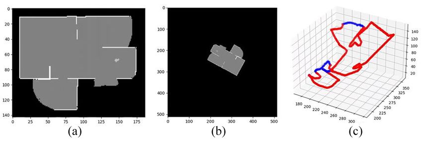
we present a novel state representation method based on 4D Fig. 1. The example of 4D point-clouds-like information. (a) shows a map
point-clouds-like information, including the locations, frontier, example in HouseExpo, where the black, gray, and white areas denote
unknown space, free space, and obstacle space, respectively. (b) shows the
and distance information. We also design a neural network that
global map in our algorithm, where the map is obtained by homogeneous
can process these 4D point-clouds-like information and generate transformations. The map’s center is the robot start location, and the map’s
the estimated value for each frontier. Then this neural network x-coordinate is the same as the robot start orientation. (c) shows the 4D
is trained using the typical reinforcement learning framework. point-clouds-like information generated based on the global map. The x,
We test the performance of our proposed method by comparing y, z coordinate denote x location, y location and distance information,
it with other five methods and test its scalability on a map that respectively. The color denotes frontier information, where red denotes
is much larger than maps in the training set. The experiment obstacles and blue denotes frontiers.
results demonstrate that our proposed method needs shorter
average traveling distances to explore whole environments and path. Many approaches have been proposed to consider more
can be adopted in maps with arbitrarily sizes.
performance metrics (i.e. information gain, etc.) [4], [5], [6].
I. I NTRODUCTION However, these approaches are designed and evaluated in a
limited number of environments. Therefore, they may fail to
Robot exploration problem is defined as making a robot or generalize to other environments whose layouts are different.
multi-robots explore unknown cluttered environments (i.e., Compared with these classical methods, machine learning-
office environment, forests, ruins, etc.) autonomously with based methods exhibit the advantages of learning from
specific goals. The goal can be classified as: (1) Maximizing various data. Deep Reinforcement Learning (DRL), which
the knowledge of the unknown environments, i.e., acquiring uses a neural network to approximate the agent’s policy
a map of the world [1], [2]. (2) Searching a static or moving during the interactions with the environments [7], gains more
object without prior information about the world. While and more attention in the application of games [8], robotics
solving the exploration problems with the second goal can [9], etc. When applied to robot exploration problems, most
combine the prior information of the target object, such as research works [10], [11] design the state space as the form
the semantic information, it also needs to fulfill the first goal. of image and use Convolution Neural Networks (CNN). For
The frontier-based methods [3], [4] have been widely example, in [10], CNN is utilized as a mapping from the
used to solve the robot exploration problem. [3] adopts a local observation of the robot to the next optimal action.
greedy strategy, which may lead to an inefficient overall However, the size of CNN’s input images is fixed, which
results in the following limitations: (1) If input images
*This work is supported by Shenzhen Key Laboratory of Robotics Percep-
tion and Intelligence (ZDSYS20200810171800001), Southern University of
represent the global information, the size of the overall
Science and Technology, Shenzhen 518055, China. (Corresponding author: explored map needs to be pre-defined to prevent input images
Jiankun Wang, Max Q.-H. Meng). from failing to fully containing all the map information.
1 Zhaoting Li and Jiankun Wang are with the Department
of Electronic and Electrical Engineering of the Southern
(2) If input images represent the local information, which
University of Science and Technology in Shenzhen, China, fails to convey all the state information, the recurrent neural
{lizt3@mail.,wangjk@}sustech.edu.cn networks (RNN) or memory networks need to be adopted.
2 Tingguang Li is with Tencent Robotics X Laboratory in Shenzhen,
Unfortunately, the robot exploration problem in this formu-
China. teaganli@tencent.com
3 Max Q.-H. Meng is with the Department of Electronic and Electrical lation requires relatively long-term planning, which is still a
Engineering of the Southern University of Science and Technology in tough problem that has not been perfectly solved.
Shenzhen, China, on leave from the Department of Electronic Engineering, In this paper, to deal with the aforementioned problems,
The Chinese University of Hong Kong, Hong Kong, and also with the
Shenzhen Research Institute of the Chinese University of Hong Kong in we present a novel state representation method, which relies
Shenzhen, China on 4D point-clouds-like information of variable size. These
information have the same data structure as point clouds            Then frontiers are defined as the boundaries between open
and consists of 2D points’ location information, and the            areas and unknown areas. The robot can constantly gain
corresponding 1D frontier and 1D distance information, as           new information about the world by moving to successive
shown in Fig.1. We also designs the corresponding training          frontiers, while the problem of selecting which frontiers
framework, which bases on the deep Q-Learning method                at a specific stage remains to be solved. Therefore, in a
with variable action space. By replacing the image obser-           frontier-based setting, solving the exploration problem is
vation with 4D point-clouds-like information, our proposed          equivalent to finding an efficient exploration strategy that
exploration model can deal with unknown maps of arbitrary           can determine the optimal frontier for the robot to explore.
size. Based on dynamic graph CNN (DGCNN) [12], which                A greedy exploration strategy is utilized in [3] to select the
is one of the typical neural network structure that process         nearest unvisited, accessible frontiers. The experiment results
point clouds information, our proposed neural network takes         in that paper show that the greedy strategy is short-sighted
4D point-clouds-like information as input and outputs the           and can waste lots of time, especially when missing a nearby
expected value of each frontier, which can guide the robot          frontier that will disappear at once if selected (this case is
to the frontier with the highest value. This neural network         illustrated in the experiment part).
is trained in a way similar to DQN in the HouseExpo                    Many DRL techniques have been applied into the robot
environment [13], which is a fast exploration simulation            exploration problem in several previous works. In a typical
platform that includes data of many 2D indoor layouts. The          DRL framework [7], the agent interacts with the environment
experiment shows that our exploration model can achieve a           by taking actions and receiving rewards from the environ-
relatively good performance, compared with the baseline in          ment. Through this trial-and-error manner, the agent can
[13], state-of-the-art in [14], classical methods in [3], [4] and   learn an optimal policy eventually. In [17], a CNN network
a random method.                                                    is trained under the DQN framework with RGB-D sensor
A. Original Contributions                                           images as input to make the robot learn obstacle avoidance
                                                                    ability during exploration. Although avoiding obstacles is
   The contributions of this paper are threefold. First, we
                                                                    important, this paper does not apply DRL to learn the
propose a novel state representation method using 4D point-
                                                                    exploration strategy. The work in [14] combines frontier-
clouds-like information to solve the aforementioned prob-
                                                                    based exploration with DRL to learn an exploration strategy
lems in Section II. Although point clouds have been utilized
                                                                    directly. The state information includes the global occupancy
in motion planning and navigation ([15], [16]), our work is
                                                                    map, robot locations and frontiers, while the action is to
different from these two papers in two main parts: (1) We
                                                                    output the weight of a cost function that evaluates the
use point clouds to represent the global information while
                                                                    goodness of each frontier. The cost function includes distance
they represent the local observation. (2) Our action space
                                                                    and information gain. By adjusting the weight, the relative
is to select a frontier point from the frontier set of variable
                                                                    importance of each term can be changed. However, the
size, while their action space contains control commands.
                                                                    terms of the cost function rely on human knowledge and
Second, we design the corresponding state function based on
                                                                    may not be applicable in other situations. In [18], the state
DGCNN [12], and the training framework based on DQN [8].
                                                                    space is similar to the one in [14], while the action is to
The novelty is that our action space’s size is variable, which
                                                                    select a point from the global map. However, the map size
makes our neural network converge in a faster way. Third,
                                                                    can vary dramatically from one environment to the next. It
we demonstrate the performance of the proposed method on
                                                                    losses generality when setting the maximum map size before
a wide variety of environments, which the model has not
                                                                    exploring the environments.
seen before, and includes maps whose size is much larger
than maps in the training set.                                         In [10] and [11], a local map, which is centered at the
   The remainder of this paper is organized as follows. We          robot’s current location, is extracted from the global map to
first introduce the related work in Section II. Then we             represent current state information. By using a local map,
formulate the frontier-based robot exploration problem and          [10] trains the robot to select actions in “turn left, turn right,
DRL exploration problem in Section III. After that, the             move forward”, while [11] learns to select points in the free
framework of our proposed method are detailed in Section            space of the local map. Local map being state space can
IV. In Section V, we demonstrate the performance of our             eliminate the limitation of global map size, but the current
proposed method through a series of simulation experiments.         local map fails to contain all the information. In [10], the
At last, we conclude the work of this paper and discuss             robot tends to get trapped in an explored room when there is
directions for future work in section VI.                           no frontier in the local map, because the robot has no idea
                                                                    where the frontiers are. The training process in [11] needs
                     II. R ELATED W ORK                             to drive the robot to the nearest frontier when the local map
   In [3], the classical frontier method is defined, where          contains no frontier information, although a RNN network
an occupancy map is utilized in which each cell is placed           is integrated into their framework. This human intervention
into one of three classes: open, unknown and occupied.              adopts a greedy strategy and can not guarantee an optimal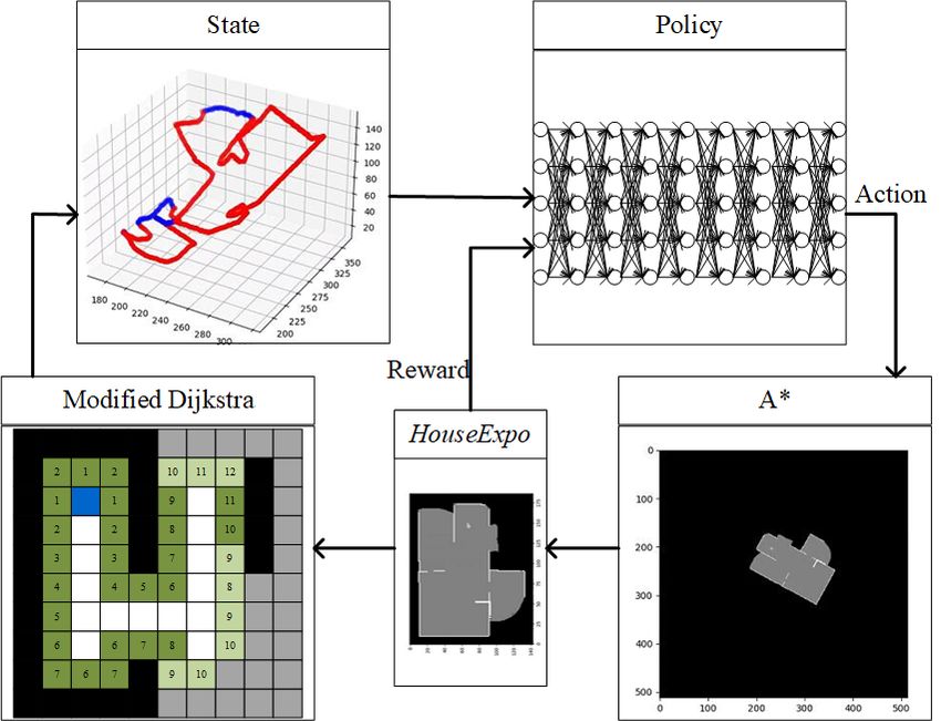
or near-optimal solution. When utilizing local observations,
the robot exploration problem requires the DRL approach to
have a long-term memory. Neural map in [19] is proposed
to tackle simple memory architecture problems in DRL. Be-
sides, Neural SLAM in [20] embeds traditional SLAM into
attention-based external memory architecture. However, the
memory architectures in [19] and [20] are based on the fixed
size of the global map. It is difficult to be applied to unknown
environments whose size may be quite large compared with
maps in training sets. Unlike the aforementioned methods,
our method uses the 4D point-clouds-like information to
represent the global state information, which does not suffer
from both the map size limitation and the simple memory
problem. As far as we know, our method is the first to apply
point clouds to robot exploration problems. Therefore, we
also design a respective DRL training framework to map the         Fig. 2.     The framework of the proposed method, which consists of
exploration strategy directly from point clouds.                   five components: (a) A simulator adopted from HouseExpo [13], which
                                                                   receives and executes a robot movement command and outputs the new
                                                                   map in HouseExpo coordinate; (b) The modified Dijkstra algorithm to
               III. P ROBLEM F ORMULATION                          extract the contour of the free space; (c) The state represented by 4D point-
   Our work aims to develop and train a neural network             clouds-like information; (d) The policy network which processes the state
                                                                   information and estimates the value of frontiers; (e) The A* algorithm that
that can take 4D point-clouds-like information as input and        finds a path connecting the current robot location to the goal frontier and
generate efficient policy to guide the exploration process of a    a simple path tracking algorithm that generates the corresponding robot
robot equipped with a laser scanner. The network should take       movement commands.
into account the information about explored areas, occupied
areas, and unexplored frontiers. In this paper, the robot          a 4-dimensional point cloud set with n points, denoted by
exploration problem is to make a robot equipped with a             Xt = {xt1 , ..., xtn } ⊂ R4 . Each point contains 4D coordinates
limited-range laser scanner explore unknown environments           xti = (xi , yi , bi , di ), where xi , yi denotes the location of the
autonomously.                                                      point, di denotes the distance from the point to the robot
                                                                   location without collision, bi ∈ {0, 1} denotes whether point
A. Frontier-based Robot Exploration Problem                        (xi , yi ) in Mt belongs to frontier or not.
   In the robot exploration problem, a 2D occupancy map is
most frequently adopted to store the explored environment          B. DRL exploration formulation
information. Define the explored 2D occupancy map at step             The robot exploration problem can be formulated as a
t as Mt . Each grid in Mt can be classified into the following     Markov Decision Process (MDP), which can be modeled
three states: free grid Mt , occupied grid Et , and unknown        as a tuple (S, A, T , R, γ). The state space S at step t is
grid Ut . According to [3], frontiers Ft are defined as the        defined by 4D point cloud Xt , which can be divided into
boundaries between the free space Et and unknown space             frontier set Ft and obstacle set Ot . The action space At
Ut . Many existing DRL exploration frameworks learn a              at step t is the frontier set Ft , and the action is to select a
mapping from Mt and Ft to robot movement commands                  point ft from Ft , which is the goal of the navigation module
which can avoid obstacles and navigate to specific locations.      implemented by A∗ [21]. When the robot take an action
Although this end-to-end framework has a simple structure,         ft from the action space, the state Xt will transit to state
it is difficult to train. Instead, our method learns a policy      Xt+1 according to the stochastic state transition probability
network that can directly determine which frontier to explore,     T (Xt , ft , Xt+1 ) = p(Xt+1 |Xt , ft ). Then the robot will
which is similar to [14] and [18]. At step t, a target frontier    receive an immediate reward rt = R(Xt , ft ). The discount
is selected from Ft based on an exploration strategy and           factor γ ∈ [0, 1] adjusts the relative importance of immediate
current explored map Mt . Once the change of the explored          and future reward. The objective of DRL algorithms is to
map is larger than the threshold, the robot is stopped, and        learn a policy π(ft |Xt ) that can select actions to maximize
the explored map at step t + 1 Mt+1 is obtained. By moving         the expected reward, which is defined as the accumulated
to selected frontiers constantly, the robot will explore more      γ−discounted rewards over time.
unknown areas until no accessible frontier exists.                    Because the action space varies according to the size of
   Because Mt can be represented as an image, it is com-           frontier set Ft , it is difficult to design a neural network that
monly used to directly represent the state information. As         maps the state to the action directly. The value-based RL is
explained in Section II, a novel state representation method       more suitable to this formulation. In value-based RL, a vector
with 4D point-clouds-like information is proposed instead.         of action values, which are the expected rewards after taking
The 4D point-clouds-like information at step t is defined as       actions in state Xt under policy π, can be estimated by a deep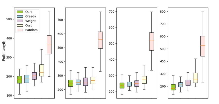
list” as Lo and Lc , respectively. The open list contains points
                                                                                 that need to be searched, while the close list contains points
                                                                                 that have been searched. Define the contour list as Lf , which
                                                                                 contains the location and the cost of points that belong to
                                                                                 frontier or obstacle. Only points in the free space of map
                                                                                 Mt are walkable. The goal of this modified algorithm is
                                                                                 to extract the contour of free space and obtain the distance
Fig. 3. The illustration of the 4D point-clouds-like information generation
process. (a) presents the map where the black, gray, white, blue points denote
                                                                                 information simultaneously. As shown in Algorithm 1, the
obstacles, unknown space, free space, and robot location. In (b), the contour    start point with the cost of zero, which is decided by the
of free space, which is denoted by green points, is generated by the modified    robot location, is added to Lo . While the open list is not
Dijkstra algorithm. The number on each point indicates the distance from
this point to the robot location. In (c), the points in the contour set are
                                                                                 empty, the algorithm repeats searching 8 points, denoted by
divided into frontier or obstacle sets, which are denoted in dark green and      pnear , adjacent to current point pcur . The differences from
light green, respectively. In (d), the 4D point-clouds-like information are      Dijkstra algorithms are: (1) If pnear belongs to occupied or
extracted from the image (c). The point clouds include location, frontier
flag, and distance information.
                                                                                 unknown space, add pcur to frontier list Lf , as shown in line
                                                                                 10 of Algorithm 1. (2) Instead of stopping when the goal is
                                         P∞                                      found, the algorithm terminates until Lo contains zero points.
Q network (DQN) Qπ (Xt , ft ; θ) = E[ i=t γ i−t ri |Xt , ft ],
                                                                                 After the algorithm ends, the contour list contains points that
where θ are the parameters of the muti-layered neural
                                                                                 are frontiers or boundaries between free space and obstacle
network. The optimal policy is to take action that has the
                                                                                 space. Points in the contour list can be classified by their
highest action value: ft∗ = argmaxft Qπ (Xt , ft ; θ). DQN
                                                                                 neighboring information into frontier or obstacle set, which
[8] is a novel variant of Q-learning, which utilizes two key
                                                                                 is shown in Fig. 3.
ideas: experience reply and target network. The DQN tends
to overestimate action values, which can be tackled by double
DQN in [22]. Double DQN select an action the same as                              Algorithm 1: Modified Dijkstra Algorithm
DQN selects, while estimate this action’s value by the target                       1: Lo ← {pstart }, Cost(pstart ) = 0;
network.                                                                            2: while Lo 6= φ do
                                                                                    3:   pcur ← minCost(Lo );
                           IV. A LGORITHM
                                                                                    4:   Lc ← Lc ∪ pcur , Lo ← Lo \pcur ;
  In this section, we present the framework of our method                           5:   for pnear in 8 points adjacent to pcur do
and illustrate its key components in detail.                                        6:     costnear = Cost(pcur ) + distance(pnear , pcur )
A. Framework Overview                                                               7:     if pnear ∈ Lc then
                                                                                    8:        continue;
   The typical DRL framework is adopted, where the robot
                                                                                    9:     else if pnear is not walkable then
interacts with the environment step by step to learn an
                                                                                   10:        Lf ← Lf ∪ pcur ;
exploration strategy. The environment in this framework is
                                                                                   11:     else if pnear ∈
                                                                                                         / Lo then
based on HouseExpo [13]. The state and action space of the
                                                                                   12:        Lo ← Lo ∪ pnear
original HouseExpo environment is the local observation
                                                                                   13:        Cost(pnear ) = costnear ;
and robot movement commands, respectively. When incorpo-
                                                                                   14:     else if pnear ∈ Lo and Cost(pnear ) > costnear
rated into our framework, HouseExpo receives a sequence
                                                                                           then
of robot movement command and outputs the global map
                                                                                   15:        Cost(pnear ) = costnear
once the change of the explored map is larger than the
                                                                                   16:     end if
threshold, which is detailed in Section III-A. As shown in
                                                                                   17:   end for
Fig. 2, the 4D point-clouds-like information can be obtained
                                                                                   18: end while
by a modified Dijkstra algorithm. After the policy network
outputting the goal point, the A∗ algorithm is implemented
to find the path connecting the robot location to the goal
                                                                                 C. Network with Point Clouds as Input
point. Then a simple path tracking algorithm is applied to
generate the sequence of robot movement commands.                                   In this section, the architecture of the state-action value
                                                                                 network with 4D point-clouds-like information as input is
B. Frontier Detection and Distance Computation                                   detailed. The architecture is modified from DGCNN in
   Computing the distances from the robot location to points                     Segmentation task [12], which proposes edge convolution
in the frontier set without collision will be time-consuming                     (EdgeConv) operation to extract the local information of
if each distance is obtained by running the A∗ algorithm                         point clouds. The EdgeConv operation includes two steps
once. Instead, we modify the Dijkstra algorithm to detect                        for each point in the input set: (1) construct a local graph
frontiers and compute distance at the same time by sharing                       including the center point and its k-nearest neighbors; (2) ap-
the search information. Denote the “open list” and “close                        ply convolution-like operations on edges which connect each
Fig. 4. The architecture of our proposed neural network. The input point clouds are classified into two categories: frontier set denoted by dark blue and
obstacle set denoted by red. The edge convolution operation EdgeConv is denoted by a light blue block, which is used to extract local features around
each point in the input set. The feature sets of frontiers and obstacles, which are generated by EdgeConv operations, are denoted by light green and
green. The MLP operation is to extract one point’s feature by only considering this point’s information. After several EdgeConv operations and one MLP
operation, a max-pooling operation is applied to generate the global information, which is shown in light yellow.

neighbor to the center point. The (Din , Dout ) EdgeConv                      be updated in a gradient decent way, after taking action ft in
operation takes the point set (N, Din ) as input and outputs                  state Xt and observing the next state Xt+1 and immediate
the feature set (N, Dout ), where Din and Dout denote the                     reward rt+1 :
dimension of input and output set, and N denotes the number
                                                                                            θt+1 = θt + α(Gt − Qπ (Xt , ft ; θt )),                  (1)
of points in the input set. Different from DGCNN and other
typical networks processing point cloud such as PointNet                      where α is the learning rate and the target Gt is defined as
[23], which have the same input and output point number,                                                                                      0

our network takes the frontier and obstacle set as input and                    Gt = rt+1 + γQπ (Xt+1 , argmax Q(Xt+1 , f ; θt ); θt ),              (2)
                                                                                                                   f
only outputs the value of points from the frontier set. The
                                                                                        0
reason for this special treatment is to decrease the action                   where θ denotes the parameter of the target network, which
                                                                                                          0
space’s size to make the network converge in a faster manner.                 is updated periodically by θ = θ.
   The network takes as input Nf + Nw points at time                             To make the estimate from our network converge to the
step t, which includes Nf frontier points and Nw obstacle                     true value, a typical DQN framework [8] can be adopted.
points, which are denoted as Ft = {xt1 , ..., xtNf } and Ot =                 For each step t, the tuple (Xt , ft , Xt+1 , rt+1 ) is saved in a
{xtNf +1 , ..., xtNf +Nw } respectively. The output is a vector of            reply buffer. The parameters can be updated by equation 1
estimated value of each action Qπ (Ft , Ot , ·; θ). The network               and 2 given the tuple sampled from the reply buffer.
architecture contains multiple EdgeConv layers and multi-                        The reward signal in the DRL framework helps the robot
layer perceptron (mlp) layers. At one EdgeConv layer, the                     know at a certain state Xt whether an action ft is appro-
feature set is extracted from the input set. Then all features                priate to take. To make the robot able to explore unknown
in this edge feature set are aggregated to compute the output                 environments successfully, we define the following reward
EdgeConv feature for each corresponding point. At a mlp                       function:
layer, the data of each point is operated on independently to
                                                                                                      t
obtain the information of one point, which is the same as the                                   rt = rarea + rft rontier + raction
                                                                                                                            t
                                                                                                                                   .                 (3)
mlp in PointNet [23]. After 4 EdgeConv layers, the outputs                                 t
                                                                              The term rarea    equals the newly discovered area at time t,
of all EdgeConv layers are aggregated and processed by a
                                                                              which is designed to encourage the robot to explore unknown
mlp layer to generate a 1D global descriptor, which encodes                                        t
                                                                              areas. The term raction    provides a consistent penalization
the global information of input points. Then this 1D global
                                                                              signal to the robot when a movement command is taken.
descriptor is concatenated with the outputs of all EdgeConv
                                                                              This reward encourages the robot to explore unknown envi-
layers. After that, points that belong to the obstacle set are
                                                                              ronments with a relatively short length of overall path. The
ignored, and the points from the frontier set are processed
                                                                              term rft rontier is designed to guide the robot to reduce the
by three mlp layers to generate scores for each point.
                                                                              number of frontiers, as defined in equation 4:
D. Learning framework based on DQN
                                                                                                         1, Nft rontier < Nft−1
                                                                                                      (
                                                                                           t                                 rontier
   As described in Section III-B, the DQN is a neural network                            rf rontier =        t             t−1
                                                                                                                                        (4)
                                                                                                        0, Nf rontier ≥ Nf rontier .
that for a given state Xt outputs a vector of action values.
The network architecture of DQN is detailed in Section                        where Nft rontier denotes the number of frontier group at time
IV-C, where the state Xt in point clouds format contains                      t.
frontier and obstacle sets. Under a given policy π(ft |Ft , Ot ),
the true value of an P   action ft in state Xt = {Ft , Ot }                    V. T RAINING D ETAILS AND S IMULATION E XPERIMENTS
                           ∞
is: Qπ (Xt , ft ; θ) ≡ E[ i=t γ i−t ri |Xt , ft ]. The target is to             In this section, we first detail the training process of
make the estimate from the frontier network converge to the                   our DRL agent. Then we validate the feasibility of our
true value. The parameters of the action-value function can                   proposed method in robot exploration problem by two sets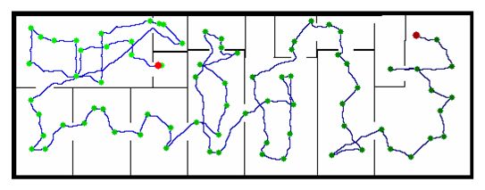
Fig. 6. Four maps for testing. The size of map1, map2, map3 and map4
Fig. 5. Some map samples from training set. The black and white pixels   is (234, 191), (231, 200), (255, 174) and (235, 174), respectively.
represent obstacle and free space respectively.

of experiments: (1) a comparison with five other exploration
methods, (2) a test of scalability where maps of larger size
compared with training set are to be explored.

A. Training Details
   To learn a general exploration strategy, the robot is trained
in the HouseExpo environment where 100 maps with
different shapes and features are to be explored. The robot
is equipped with a 2m range laser scanner with a 180 degree
field of view. The noise of laser range measurement is                   Fig. 7. The path length’s data of each method on four test maps. For each
simulated by the Gaussian distribution with a mean of 0 and              map, each method is tested for 100 times with the same randomly initialized
a standard deviation of 0.02m. As an episode starts, a map is            robot start locations.
randomly selected from the training set, and the robot start
pose, including the location and pose, is also set randomly.             32 times with a batch size equal to 1. Learning parameters
In the beginning, the circle area centered at the start location         are listed in Table 1. The training process is performed on
is explored by making the robot rotate for 360 degree. Then              a computer with Intel i7-7820X CPU and GeForce GTX
at each step, a goal frontier point is selected from the frontier        1080Ti GPU. The training starts at 2000 steps and ends after
set under the policy of our proposed method. A* algorithm                90000 update steps, which takes 72 hours.
is applied to find a feasible path connecting the current robot          B. Comparison Study
location to the goal frontier. A simple path tracking algorithm
                                                                            Besides our proposed method, we also test the perfor-
is used to find the robot commands to follow the planned
                                                                         mance of the weight tuning method in [14], a cost-based
path: moving to the nearest unvisited path point pnear , and
                                                                         method in [4], a method with greedy strategy in [3], a method
replanning the path if the distance between the robot and
                                                                         utilizing a random policy and the baseline in [13], which we
pnear is larger than a fixed threshold. An episode ends if the
                                                                         denote as the weight method, cost method, greedy method,
explored ratio of the whole map is over 95%.
                                                                         random method and baseline, respectively. To compare the
                             TABLE I                                     performance of different methods, we use 4 maps as a testing
                       PARAMETERS IN T RAINING                           set, as shown in Fig. 6. For each test map, we conduct 100
                                                                         trials by setting robot initial locations randomly for each trail.
           HouseExpo                           Training                     The random method selects a frontier point from the
    Laser range           2m        Discount factor γ         0.99       frontier set randomly. The greedy method chooses the nearest
 Laser field of view     180◦    Target network update f   4000 steps
    Robot radius        0.15m         Learning rate          0.001
                                                                         frontier point. The baseline utilizes a CNN which directly
 Linear step length      0.3m       Replay buffer size       50000       determines the robot movement commands by the current
 Angular step length      15◦       Exploration rate        15000       local observation.
    Meter2pixel            16        Learning starts         3000           The cost method evaluates the scalar value of frontiers by
                                                                         a cost function considering distance and information gain
   Some training map samples are shown in Fig. 5. The                    information.
largest size of a map in the training set is 256 by 256.
                                                                                            cost = wd + (1 − w)(1 − g),                         (5)
Because the size of state information Xt changes at each
time and batch update method requires point clouds with                  where w is the weight that adjusts the relative importance
same size, currently, it is not realistic to train the model             of costs. d and g denote the normalized distance and in-
in a batch-update way. In typical point clouds classification            formation gain of a frontier. At each step, after obtaining
training process, the size of all the point clouds data are pre-         the frontier set as detailed in Section IV-B, the k-means
processed to the same size. However, these operations will               method is adopted to cluster the points in the frontier set
change the original data’s spatial information in our method.            to find frontier centers. To reduce the runtime of computing
Instead, for each step, the network parameters are updated               information gains, we only compute the information gain
Fig. 9. The ratio of the area explored and the area of the whole map
Fig. 8. The representative exploration trials of six different methods on with respect to the current path’s length. The test map is map1 and the start
map1 with the same robot start locations and poses. The bright red denotes locations is the same as Fig. 8.
the start state and the dark red denotes the end state. The green point denotes
the locations where the robot made decisions to choose which frontiers to
explore. As the step increases, the brightness of green points becomes darker and information gain. If the computation of the information
and darker. The baseline’s result doesn’t have green points because its action gain is not accurate or another related cost exists, the weight
is to choose a robot movement command.
method fails to fully demonstrate the advantages of learning.
Instead, our proposed method can learn useful information,
for each frontier center. The information gain is computed including information gain, by learning to estimate the value
by the area of the unknown space to be explored if this of frontiers, which is the reason that our proposed method
frontier center is selected [4]. The weight in the cost method outperforms the weight method.
is fixed to 0.5, which fails to be optimal in environments Fig. 8 shows an example of the overall paths of six differ-
with different structures and features. ent methods when exploring the map1 with the same starting
The weight method can learn to adjust the value of the pose. Each episode ended once the explored ratio was more
weight in equation 5 under the same training framework as than 0.95. The proposed method explored the environment
our proposed method. The structure of the neural network with the shortest path. The explored ratio of the total map
in weight method is presented in Fig. 4, which takes the 4D according to the length of the current path is shown in Fig.
point-clouds-like information as input and outputs a scalar 9. The greedy method’s curve has a horizontal line when the
value. explored ratio is near 0.95. This is because the greedy method
We select the length of overall paths, which are recorded missed a nearby frontier which would disappear at once
after 95% of areas are explored, as the metric to evaluate if selected. However, the greedy method chose the nearest
the relative performance of the six exploration methods. The frontier instead, which made the robot travel to that missed
length of overall paths can indicate the efficiency of the frontier again and resulted in a longer path. For example,
exploration methods. The box plot in Fig. 7 is utilized to in Fig. 8, the greedy method chose to explore the point
visualize the path length’s data of each exploration method C instead of the point A, when the robot was at point B.
on four test maps. The baseline is not considered here This decision made the robot travel to the point A later, thus
because the baseline sometimes fails to explore the whole making the overall path longer. The baseline’s curve also
environment, which will be explained later. Three values exhibits a horizontal line in Fig. 9, which is quite long. The
of this metric are used to analyze the experiment results: baseline’s local observation contained no frontier information
(1) the average, (2) the minimum value, (3) the variance. when the surroundings were all explored (in the left part of
Our proposed method has the minimum average length of the environment shown in Fig. 8). Therefore, at this situation,
overall paths for all four test maps. The minimum length of the baseline could only take “random” action (i.e. travelling
the proposed method in each map is also smaller than other along the wall) to find the existing frontiers, which would
five methods. This indicates that the exploration strategy of waste lots of travelling distances and may fail to explore the
our proposed method is more effective and efficient than whole environment.
the other five methods. The random method has the largest
variance and average value for each map because it has C. Scalability Study
more chances to sway between two or more frontier groups. In this section, a map size of (531, 201) is used to test the
That is why the overall path of the random method in performance of our proposed method in larger environments
Fig. 8 is the most disorganized. The weight method has a compared with maps in the training set. If the network’s input
lower average and minimum value compared with the cost is fixed size images, the map needs to be padded into a (531,
method in all test maps, due to the advantages of learning 531) image, which is a low-efficient state representation way.
from rich data. However, the weight method only adjusts a Then a downscaling operation of the image is required to
weight value to change the relative importance of distance make the size of the image input the same as the requirement[3] B. Yamauchi, “A frontier-based approach for autonomous exploration,”
in Proceedings 1997 IEEE International Symposium on Computational
Intelligence in Robotics and Automation CIRA’97.’Towards New Com-
putational Principles for Robotics and Automation’. IEEE, 1997, pp.
146–151.
[4] H. H. González-Banos and J.-C. Latombe, “Navigation strategies for
exploring indoor environments,” The International Journal of Robotics
Research, vol. 21, no. 10-11, pp. 829–848, 2002.
[5] F. Bourgault, A. A. Makarenko, S. B. Williams, B. Grocholsky, and
H. F. Durrant-Whyte, “Information based adaptive robotic explo-
ration,” in IEEE/RSJ international conference on intelligent robots and
Fig. 10. The result of the scalability test. The map size is (531, 201). The systems, vol. 1. IEEE, 2002, pp. 540–545.
meaning of points’ color is the same as Fig. 8 [6] N. Basilico and F. Amigoni, “Exploration strategies based on multi-
criteria decision making for searching environments in rescue opera-
tions,” Autonomous Robots, vol. 31, no. 4, pp. 401–417, 2011.
of the neural network, e.g. (256,256). Although the neural [7] R. S. Sutton and A. G. Barto, Reinforcement learning: An introduction.
MIT press, 2018.
network can process the state data by downscaling, the [8] V. Mnih, K. Kavukcuoglu, D. Silver, A. A. Rusu, J. Veness, M. G.
quality of the input data decreases. Therefore, the network Bellemare, A. Graves, M. Riedmiller, A. K. Fidjeland, G. Ostrovski
fails to work once the scaled input contains much less nec- et al., “Human-level control through deep reinforcement learning,”
nature, vol. 518, no. 7540, pp. 529–533, 2015.
essary information than the original image. Fig. 10 presents [9] S. James, Z. Ma, D. R. Arrojo, and A. J. Davison, “Rlbench: The
the overall path generated by our method without down- robot learning benchmark & learning environment,” IEEE Robotics
scaling the map size. Our proposed method, which takes and Automation Letters, vol. 5, no. 2, pp. 3019–3026, 2020.
[10] D. Zhu, T. Li, D. Ho, C. Wang, and M. Q. . Meng, “Deep re-
point clouds as input, has better robustness in maps with inforcement learning supervised autonomous exploration in office
large scales because of the following two reasons. First, we environments,” in 2018 IEEE International Conference on Robotics
incorporate the distance information into point clouds, which and Automation (ICRA), 2018, pp. 7548–7555.
[11] F. Chen, S. Bai, T. Shan, and B. Englot, “Self-learning exploration
can help neural networks learn which part of point clouds and mapping for mobile robots via deep reinforcement learning,” in
are walkable. Although the image representation can also Aiaa scitech 2019 forum, 2019, p. 0396.
have a fourth channel as distance information, the scaling [12] Y. Wang, Y. Sun, Z. Liu, S. E. Sarma, M. M. Bronstein, and J. M.
Solomon, “Dynamic graph cnn for learning on point clouds,” Acm
operation can make some important obstacles or free points Transactions On Graphics (tog), vol. 38, no. 5, pp. 1–12, 2019.
disappear, which changes the structure of the map. Secondly, [13] T. Li, D. Ho, C. Li, D. Zhu, C. Wang, and M. Q.-H. Meng,
the number of pixels in an image increases exponentially as “Houseexpo: A large-scale 2d indoor layout dataset for learning-based
algorithms on mobile robots,” arXiv preprint arXiv:1903.09845, 2019.
the size of the image increase. The number of points in point [14] F. Niroui, K. Zhang, Z. Kashino, and G. Nejat, “Deep reinforcement
clouds equals the number of pixels that represent an obstacle learning robot for search and rescue applications: Exploration in
or frontier in a map, which is not an exponential relation unknown cluttered environments,” IEEE Robotics and Automation
Letters, vol. 4, no. 2, pp. 610–617, 2019.
unless all the pixels in a map are obstacles or frontiers. [15] F. Leiva and J. Ruiz-del Solar, “Robust rl-based map-less local
planning: Using 2d point clouds as observations,” IEEE Robotics and
Automation Letters, vol. 5, no. 4, pp. 5787–5794, 2020.
VI. C ONCLUSIONS A ND F UTURE W ORK [16] R. Strudel, R. Garcia, J. Carpentier, J. Laumond, I. Laptev, and
C. Schmid, “Learning obstacle representations for neural motion
In this paper, we present a novel state representation planning,” Proceedings of Conference on Robot Learning (CoRL),
2020.
method using 4D point-clouds-like information and design [17] L. Tai and M. Liu, “A robot exploration strategy based on q-learning
the framework to learn an efficient exploration strategy. Our network,” in 2016 IEEE International Conference on Real-time Com-
proposed method can solve the problems that come with puting and Robotics (RCAR), 2016, pp. 57–62.
[18] H. Li, Q. Zhang, and D. Zhao, “Deep reinforcement learning-based
using images as observations. The experiments demonstrate automatic exploration for navigation in unknown environment,” IEEE
the effectiveness of our proposed method, compared with transactions on neural networks and learning systems, vol. 31, no. 6,
other five commonly used methods. For the future work, pp. 2064–2076, 2019.
[19] E. Parisotto and R. Salakhutdinov, “Neural map: Structured memory
other network structures and RL algorithms can be modified for deep reinforcement learning,” in International Conference on
and applied to the robot exploration problem with point Learning Representations, 2018.
clouds as input. The converge speed of training may also be [20] J. Zhang, L. Tai, J. Boedecker, W. Burgard, and M. Liu, “Neural
slam: Learning to explore with external memory,” arXiv preprint
improved by optimizing the training techniques. Besides, the arXiv:1706.09520, 2017.
multi-robot exploration problem may also use point clouds [21] N. J. N. Hart, Peter E. and B. Raphael, “A formal basis for the heuristic
to represent the global information. determination of minimum cost paths,” IEEE transactions on Systems
Science and Cybernetics, vol. 4, no. 2, pp. 100–107, 1968.
[22] H. v. Hasselt, A. Guez, and D. Silver, “Deep reinforcement learning
R EFERENCES with double q-learning,” in Proceedings of the Thirtieth AAAI Confer-
ence on Artificial Intelligence, ser. AAAI’16. AAAI Press, 2016, p.
2094–2100.
[1] S. Thrun, “Probabilistic robotics,” Communications of the ACM, [23] C. R. Qi, H. Su, K. Mo, and L. J. Guibas, “Pointnet: Deep learning
vol. 45, no. 3, pp. 52–57, 2002. on point sets for 3d classification and segmentation,” in Proceedings
[2] S. Oßwald, M. Bennewitz, W. Burgard, and C. Stachniss, “Speeding- of the IEEE conference on computer vision and pattern recognition,
up robot exploration by exploiting background information,” IEEE 2017, pp. 652–660.
Robotics and Automation Letters, vol. 1, no. 2, pp. 716–723, 2016.You can also read