Level 2B Radar-only Cloud Water Content (2B-CWC-RO) Process Description Document
←
→
Page content transcription
If your browser does not render page correctly, please read the page content below
CloudSat Project
A NASA Earth System Science Pathfinder Mission

Level 2B Radar-only Cloud Water Content
(2B-CWC-RO) Process Description Document
Version: 5.1

Date: 21 October 2007

Questions concerning the document and proposed changes should be addressed to
     Richard Austin
     austin@atmos.colostate.edu
     +1 970 491 8587

                                              1
CONTENTS 2
Contents
1 Introduction 3
2 Algorithm Theoretical Basis—Liquid Water Content 4
2.1 Forward Model and Measurements . . . . . . . . . . . . . . . . . . . . . . . . . . . . 4
2.1.1 Physics of the Forward Model . . . . . . . . . . . . . . . . . . . . . . . . . . 4
2.1.2 Departures From the Lognormal Distribution . . . . . . . . . . . . . . . . . . 6
2.1.3 Mixed phase and multi-layered clouds . . . . . . . . . . . . . . . . . . . . . . 6
2.2 Retrieval Algorithm . . . . . . . . . . . . . . . . . . . . . . . . . . . . . . . . . . . . 7
2.2.1 State and Measurement Vectors . . . . . . . . . . . . . . . . . . . . . . . . . 7
2.2.2 Forward Model and Parameters . . . . . . . . . . . . . . . . . . . . . . . . . 8
2.2.3 A Priori Data and Covariance . . . . . . . . . . . . . . . . . . . . . . . . . . 9
2.2.4 Convergence and Quality Control . . . . . . . . . . . . . . . . . . . . . . . . 10
3 Algorithm Theoretical Basis—Ice Water Content 11
3.1 Forward Model and Measurements . . . . . . . . . . . . . . . . . . . . . . . . . . . . 11
3.1.1 Physics of the Forward Model . . . . . . . . . . . . . . . . . . . . . . . . . . 11
3.1.2 Algorithm refinements: correction for Lorenz-Mie effects . . . . . . . . . . . 12
3.1.3 Further possible algorithm refinements: correction for density effects . . . . . 13
3.1.4 Departures from the Lognormal Distribution . . . . . . . . . . . . . . . . . . 14
3.1.5 Mixed phase and multi-layered clouds . . . . . . . . . . . . . . . . . . . . . . 14
3.2 Retrieval Algorithm . . . . . . . . . . . . . . . . . . . . . . . . . . . . . . . . . . . . 14
3.2.1 State and Measurement Vectors . . . . . . . . . . . . . . . . . . . . . . . . . 14
3.2.2 Forward Model and Parameters . . . . . . . . . . . . . . . . . . . . . . . . . 15
3.2.3 A Priori Data and Covariance . . . . . . . . . . . . . . . . . . . . . . . . . . 15
3.2.4 Convergence and Quality Control . . . . . . . . . . . . . . . . . . . . . . . . 16
4 Algorithm Theoretical Basis—Cloud Water Content 17
5 Algorithm Inputs 19
5.1 CloudSat . . . . . . . . . . . . . . . . . . . . . . . . . . . . . . . . . . . . . . . . . 19
5.1.1 CloudSat 2B-GEOPROF Data . . . . . . . . . . . . . . . . . . . . . . . . . . 19
5.1.2 CloudSat 2B-CLDCLASS Data . . . . . . . . . . . . . . . . . . . . . . . . . 19
5.2 Ancillary (Non-CloudSat) . . . . . . . . . . . . . . . . . . . . . . . . . . . . . . . . 19
5.2.1 CloudSat ECMWF-AUX Data . . . . . . . . . . . . . . . . . . . . . . . . . . 19
6 Algorithm Summary 20
7 Data Product Output Format 23
8 Changes since version 5.0 231 INTRODUCTION 3
1 Introduction
The CloudSat Radar-Only Cloud Water Content Product (2B-CWC-RO) contains retrieved estimates
of cloud liquid and ice water content, effective radius, and related quantities for each radar profile
measured by the Cloud Profiling Radar on CloudSat. Retrievals are performed separately for the
liquid and ice phases; the two sets of results are then combined in a simple way to obtain a composite
profile that is consistent with the input measurements.
This radar-only (RO) product uses measured radar reflectivity factor as the sole input from remote
sensing instruments. A similar CloudSat standard data product, 2B-CWC-RVOD, uses estimates of
visible optical depth (from the CloudSat 2B-TAU product) together with the radar measurements to
more tightly constrain the retrievals, which should result in more accurate results. However, retrievals
of visible optical depth are difficult or impossible in many cases, due to the complexity of the targets
and the simplifying assumptions made necessary by the data volumes associated with an operational
satellite. Therefore, the CloudSat retrievals are produced in both radar-only (RO) and radar-visible
optical depth (RVOD) versions, allowing the user to work with the generally available RO data, which
are supplemented by the RVOD solutions where possible. The 2B-CWC-RVOD product should be
released a few months after the RO product.
The CWC algorithm creates a composite profile from separate ice and liquid water retrievals. Both
of these retrievals assume that the radar profile is due to a single phase of water, that is, that the entire
profile consists of either liquid or ice, but not both. The resulting separate liquid and ice profiles
are then combined using a simple scheme based on temperature as reported by an ECMWF model.
While the combination algorithm results in a mixture of ice and liquid phases over that part of the
vertical profile that has the proper temperature range, the user should be aware that the retrieval does
not attempt to retrieve mixed-phase cloud properties directly. Improvements are in the planning stages
to better handle the retrieval of mixed-phase cloud.
This document describes the algorithms that have been implemented in Release 4 (R04) of the
2B-CWC-RO product (algorithm version 5.1). For each radar profile, the algorithms will
• Examine the cloud mask in 2B-GEOPROF to determine which bins in the column contain cloud,
• Examine the 2B-CLDCLASS product to determine if any cloudy bins have an undetermined or
invalid cloud type (indicating a problematic profile),
• Assign a priori values to the liquid and ice particle size distribution parameters in each cloudy
bin based on climatology, temperature, or other criteria,
• Using the a priori values and radar measurements from 2B-GEOPROF, retrieve liquid and ice
particle size distribution parameters for each cloudy bin. Derive effective radius, water content,
and related quantities from the retrieved size distributions for both liquid and ice phases, together
with associated uncertainties,
• Create a composite profile by using the retrieved ice properties at temperatures colder than
−20◦ C, the retrieved liquid properties at temperatures warmer than 0◦ C, and a linear combination
of the two in intermediate temperatures,
• For each of these estimates, calculate uncertainties and covariance matrices.2 ALGORITHM THEORETICAL BASIS—LIQUID WATER CONTENT 4
2 Algorithm Theoretical Basis—Liquid Water Content
The liquid cloud retrieval algorithm is a modification of the method described in Austin and Stephens
(200X). [A previous version of the algorithm is described in Austin and Stephens (2001).] Condensed
versions of the descriptions of the forward model and retrieval formulation are given here and in the
following section, together with a description of modifications specific to the operational CloudSat
algorithm.
2.1 Forward Model and Measurements
The retrieval uses active remote sensing data together with a priori data to estimate the parameters
of the particle size distribution in each bin containing cloud. Radar measurements provide a vertical
profile of cloud backscatter; the measured backscatter value and a cloud mask (indicating the likelihood
that a particular radar bin contains cloud) are obtained from 2B-GEOPROF.
2.1.1 Physics of the Forward Model
The forward model developed for the retrieval assumes a lognormal size distribution of cloud droplets:
− ln2 (r/rg )
" #
NT
N (r) = √ exp 2
, (1)
2πσlog r 2σlog
where NT is the droplet number density, r is the droplet radius, and rg , σlog , and σg are defined by
ln rg = ln r,
σlog = ln σg ,
σg2 = (ln r − ln rg )2 ,
where rg is the geometric mean radius, σlog is the distribution width parameter, σg is the geometric
standard deviation, ln indicates the natural (base e) logarithm, and the overbar indicates the arithmetic
mean. The distribution in (1) is fully specified by three parameters: NT , σlog , and rg . The liquid water
content LWC and the effective radius re are defined in terms of moments of the size distribution:
Z ∞ 4
LWC = ρw N (r) πr3 dr, (2)
0 3
R∞
N (r)r3 dr
re = R0∞ , (3)
0 N (r)r2 dr
where ρw is the density of water.
For clouds having negligible drizzle or precipitation, cloud droplets are sufficiently small to be mod-
eled as Rayleigh scatterers at the CloudSat radar wavelength and sufficiently large that their extinction
efficiency approaches 2 for visible wavelengths. These assumptions yield the following definitions of
radar reflectivity factor Z and visible extinction coefficient σext :
Z ∞
Z = 64 N (r)r6 dr, (4)
02 ALGORITHM THEORETICAL BASIS—LIQUID WATER CONTENT 5
Z ∞
σext = 2 N (r)πr2 dr. (5)
0
Using (1) for the size distribution in (2) through (5) gives the following equations for the various cloud
properties:
4π 9 2
3
LWC = NT ρw rg exp σlog , (6)
3 2
5 2
re = rg exp σlog , (7)
2
Z = 64NT rg6 exp(18σlog 2
), (8)
σext = 2πNT rg2 exp(2σlog
2
). (9)
All of these properties are functions of position in the cloud column; we can therefore write LWC(z),
re (z), Z(z), and σext (z).
The visible optical depth τ is calculated by integrating the visible extinction coefficient through the
cloud column: Z ztop
τ= σext (z) dz, (10)
zbase
where zbase and ztop are the cloud base and top, respectively. Equations (6) through (10) express the
intrinsic properties of the cloud as functions of the parameters of the assumed drop size distribution;
they form the basis of the retrieval. LWC and re are the quantities we seek to retrieve, and values of
Z are related to our measurements. We may also specify LWP, the columnar liquid water content or
liquid water path, Z ztop
LWP = LWC(z) dz. (11)
zbase
The scattered energy received by the radar from particles at a given range will be attenuated in
both directions by cloud particles between that range and the radar receiver. (It will also experience
gaseous attenuation, primarily by water vapor; this attenuation is provided as a separate variable in the
2B-GEOPROF product and is therefore not considered here.) The measured reflectivity factor Z 0 will
be reduced from the intrinsic reflectivity factor Z according to the following expression:
Z
0 0 0
Z (z) = Z(z) exp −2 σabs (z ) dz , (12)
path
where the path integral is over the portion of the cloud between z and the radar. The absorption
coefficient at the radar frequency σabs is given by
Z ∞
σabs (z) = N (r, z)Cabs (r) dr, (13)
0
where N (r, z) is the particle size distribution at z and Cabs is the absorption cross section as a function
of particle radius r. (Scattering effects are much smaller than absorption effects at the radar wave-
length, so we approximate the attenuation as being purely due to absorption.)
Assuming the cloud droplets are sufficiently small to be modeled as spherical droplets, we may use
Mie theory to obtain an expression for Cabs :
8π 2 r3
Cabs = Im{−K}, (14)
λ2 ALGORITHM THEORETICAL BASIS—LIQUID WATER CONTENT 6
where λ is the radar wavelength and K is given by
m2 − 1
K= , (15)
m2 + 2
where m is the complex index of refraction of the droplet material (water) at the radar frequency
and ambient temperature. Using the lognormal distribution in (1), the absorption coefficient in (13)
becomes
8π 2 NT 9 2
3
σabs = Im{−K}rg exp σlog , (16)
λ 2
where the z dependence is suppressed for clarity.
Assuming that a lognormal distribution is appropriate, the cloud microphysics are fully described
by specification of the three lognormal distribution parameters NT (z), σlog (z), and rg (z). Liquid water
content and effective radius may then be obtained through (6) and (7). Because the measured data are
limited to a single radar reflectivity factor Z 0 for each radar resolution bin, we rely on a priori data
to constrain the retrieval where the measurements cannot, allowing the retrieved solution to be con-
sistent with the measurements without imposing fixed values of (e.g.) particle number concentration
through the cloud column. The optimal estimation technique employed in this retrieval is described in
section 2.2.
2.1.2 Departures From the Lognormal Distribution
The retrieval assumes a lognormal distribution of liquid cloud droplets, as given in (1). Departures
from this distribution will degrade the accuracy of the retrieval. One source of departure from this an-
alytic distribution is the presence of drizzle or rain within the cloud. Detection criteria for the presence
of drizzle or rain are under development. (The current procedure identifies drizzle or precipitation for
any case where Z 0 ≥ −15 dBZ.) Drizzle/precipitation is indicated in the output by setting a flag in the
status variable, but the algorithm is still run as normal, producing output values (unless the solution
diverges). The flag serves as an indicator that the solution is likely unreliable due to a violation of
the lognormal distribution assumption. In practice, the presence of any significant precipitation causes
the retrieval to fail to converge, resulting in an error condition. Retrieval of cloud properties in the
presence of precipitation is a difficult problem due to the sensitivity of the radar to precipitation-sized
particles. Better handling of this case is a high priority for future development of this product.
2.1.3 Mixed phase and multi-layered clouds
The liquid water content retrieval algorithm assumes that the entire cloud column is composed of
liquid water droplets. (The retrievals used in 2B-CWC-RO consider only one phase of water at a
time.) Because we have no independent means of determining the particle phase in a given radar bin,
a simple partition scheme is employed to create a composite ice/liquid profile, discarding the retrieved
liquid properties in portions of the profile deemed to consist purely of ice. The partition scheme is
described in section 4.2 ALGORITHM THEORETICAL BASIS—LIQUID WATER CONTENT 7
2.2 Retrieval Algorithm
The retrieval uses an approach described by Rodgers (1976, 1990, 2000) and Marks and Rodgers
(1993), where a vector of measured quantities y (here, radar reflectivities) is related to a state vector of
unknowns x (geometric mean radii, number density, and distribution width parameter) by the forward
model F:
y = F(x) + y , (17)
where y represents measurement errors. Rodgers (1976) described an optimal-estimation technique
in which a priori profiles are used as virtual measurements, serving as a constraint on the retrieval. An
a priori profile xa is specified based on likely or statistical values of the state vector elements, together
with an a priori covariance matrix Sa representing the variability or uncertainty of this profile and the
covariance between various profile elements.
The retrieval algorithm obtains the optimal solution by minimizing a cost function Φ that represents
a weighted sum of the measurement vector-forward model difference and the state vector-a priori
difference:
Φ = (x̂ − xa )T S−1 T −1
a (x̂ − xa ) + [y − F(x̂)] Sy [y − F(x̂)]. (18)
The solution is obtained by iteration using successive estimates of the x vector and the K matrix
(K = ∂F/∂x). These quantities are also used to provide information on convergence, the quality
of the solution, and the amounts and sources of retrieval uncertainty. The various input and output
quantities are described here; see Austin and Stephens (200X) for a more detailed description.
2.2.1 State and Measurement Vectors
The state vector x is the vector of unknown cloud parameters to be retrieved. For a cloud reflectivity
profile consisting of p cloudy bins, the state vector will have n = 3p elements:
rg (z1 )
..
.
rg (zp )
NT (z1 )
..
x=
. ,
(19)
NT (zp )
σlog (z1 )
..
.
σlog (zp )
where rg (zi ), NT (zi ), and σlog (zi ) are the geometric mean radius, droplet number concentration, and
distribution width parameter for height zi (we shall often write these as rgi , etc.). Here z1 is the height
of the radar resolution bin at cloud base; zp is at the top of the cloud profile. Units are selected to
keep the numerical values within similar orders of magnitude: µm for rg and cm−3 for NT (σlog is
dimensionless).2 ALGORITHM THEORETICAL BASIS—LIQUID WATER CONTENT 8
The RO measurement vector y is composed of m = p elements for a cloud profile of p cloudy bins:
Z 0 (z1 )
dB.
..
y=
,
(20)
0
ZdB (zp )
0 0
where ZdB (zi ) is the measured radar reflectivity factor for height zi (often written as ZdB i
). Reflectivity
6 −3
factor Z is specified in units of mm m . To reduce the large dynamic range of the reflectivity
variable and to make the model more linear, Z has been converted to a logarithmic variable ZdB by the
transform ZdB = 10 log Z, where ZdB has units of dBZ and log indicates the base 10 logarithm.
The measurement error covariance matrix S gives a measure of the uncertainties in the measure-
ment vector and of correlations between the errors of the individual elements. In the present retrieval,
it is assumed that the elements of y have independent errors given as follows:
σZ2 0 0 ··· 0
dB1
.. ..
0 . 0 .
S =
.. ...
,
(21)
. 0 0
0 ··· 0 σZ2 0
dBp
where σZdB0 is the standard deviation of the measured radar reflectivity factor in dBZ (i.e., the uncer-
i
tainty in the measured radar reflectivity values from whatever source [noise, calibration error, etc.],
usually a fixed number for a given radar).
2.2.2 Forward Model and Parameters
The forward model F(x) relates the state vector x to the measurement vector y. F therefore has the
same dimension as y:
0
ZdB FM
(z1 )
F(x) =
..
, (22)
.
0
ZdBFM (zp )
where the individual elements are given by the following expressions:
0
ZdB FM
(zi ) =
(
10 log 64NT rg6i exp(18σlog
2
)
−16π 2 NT
"
× exp Im{−K}
λ
p #)
9 2
3
X
× exp σlog ∆z rgj , i = 1, . . . , p − 1 (23)
2 j=i+1
h i
0
ZdB FM
(zi ) = 10 log 64NT rg6i exp(18σlog
2
) , i=p (24)2 ALGORITHM THEORETICAL BASIS—LIQUID WATER CONTENT 9
(The symbol ∆z represents the thickness of a radar range bin.) The subscript FM is a reminder that
these quantities are calculated from elements of x according to the forward model equations (23) and
(24), as opposed to the elements of the y vector, which are measured quantities. The form of (23) and
(24) assumes that the radar is above the cloud looking down; again, z1 is the lowest bin in the cloud
and zp is the highest.
2.2.3 A Priori Data and Covariance
A priori data for the retrieval are selected based on collections of microphysical measurements of
related cloud types. Reference values for each of these categories are obtained from a database of
cloud microphysical parameters (e.g., Miles et al. 2000). The selected values for each radar profile are
included in the product output. The a priori vector xa is specified as follows:
rga (z1 )
..
.
rga (zp )
NT a (z1 )
..
xa = . (25)
.
NT a (zp )
σloga (z1 )
..
.
σloga (zp )
We also specify an a priori error covariance matrix Sa :
σr2ga1 0 ··· 0 ··· 0 0 ··· 0
.. .. .. .. .. .. ..
0 . 0 . . . . . .
..
. 0 σr2gap 0 ··· 0 0 ··· 0
.. .. .. ..
2
0 ··· 0 σN Ta
0 . . . .
1
.. .. .. .. .. ..
Sa = . ··· . 0 . 0 . . . . (26)
.. ..
2
··· ···
0 0 0 σN T ap
0 . .
..
0 ··· 0 ··· ··· 0 σσ2loga 0 .
1
.. .. ..
. ··· . ··· ··· ··· 0 . 0
2
0 ··· 0 ··· ··· ··· ··· 0 σσloga
p
Adjustment of the a priori parameters xa and uncertainties Sa in future versions may allow cus-
tomization of the retrieval for different cloud types, generation regimes (e.g., continental or maritime),
and geographic areas (tropical, midlatitude, etc.).2 ALGORITHM THEORETICAL BASIS—LIQUID WATER CONTENT 10
2.2.4 Convergence and Quality Control
The state vector x̂ is obtained by iteration. The a priori values xa are used as the initial value of x̂.
Convergence of the solution is determined using a test with the following form:
∆x̂T S−1
x ∆x̂
n, (27)
where n is the dimension of the x̂ vector, i.e. the number of cloudy radar bins times three. The error
covariance matrix Sx of the retrieved state vector x̂ is given by
Sx = (S−1 T −1 −1
a + K Sy K) . (28)
Elements of the Sx matrix give the covariance between elements of the retrieved state vector x̂; diag-
onal elements of Sx are variances in the elements of x̂ and give a measure of the uncertainty in the
retrieval. For this retrieval, we specify the criterion for “much less than” in (27) such that
∆x̂T S−1
x ∆x̂ < 0.01n. (29)
After the iteration converges, we seek a test that shows the goodness of fit of the retrieved values to
the measurements. Using the hypothesis that the fit to the measurements (including the a priori virtual
measurements) is consistent with the measurement uncertainties (including the a priori uncertainties),
Marks and Rodgers (1993) used the following χ2 :
χ2 = [y − F(x̂)]T S−1 T −1
y [y − F(x̂)] + (xa − x̂) Sa (xa − x̂). (30)
This quantity should follow a χ2 distribution with m degrees of freedom (n parameters fitted to m + n
measurements, where n and m are the dimensions of the x̂ and y vectors, respectively). Marks and
Rodgers (1993) noted that a typical value of χ2 for a “moderately good retrieval” is m.
As currently implemented, the retrieval rejects profiles where any element of the x̂ vector becomes
negative during any iteration. (This is infrequent.) Profiles are also rejected if the measured reflec-
tivity factor exceeds a specified maximum level (i.e., it is unphysical) or if the radar information is
unavailable.3 ALGORITHM THEORETICAL BASIS—ICE WATER CONTENT 11
3 Algorithm Theoretical Basis—Ice Water Content
The retrieval algorithm is described in Austin et al. (200X); an earlier version is described by Benedetti
et al. (2003). Condensed versions of the descriptions of the forward model and retrieval formulation
are given here and in the following section, together with a description of modifications specific to the
operational CloudSat algorithm.
3.1 Forward Model and Measurements
Like the liquid cloud retrieval, this retrieval uses active remote sensing data together with a priori
data to estimate the parameters of the particle size distribution in each bin containing cloud. Radar
measurements provide a vertical profile of cloud backscatter; the measured backscatter value and a
cloud mask (indicating the likelihood that a particular radar bin contains cloud) are obtained from
2B-GEOPROF.
3.1.1 Physics of the Forward Model
The forward model developed for the retrieval assumes a lognormal size distribution of ice crystals:
− ln2 (D/Dg )
" #
NT
N (D) = √ exp 2
, (31)
2πσlog D 2σlog
where NT is the ice particle number concentration, D is the diameter of an equivalent mass ice sphere,
Dg is the geometric mean diameter, and σlog is the width parameter. The distribution in (31) is fully
specified by three parameters: NT , Dg , and σlog . The ice water content (IWC) and the effective radius
re are defined in terms of moments of the size distribution:
Z ∞
π
IWC = ρi N (D)D3 dD (32)
0 6
1 ∞ N (D)D3 dD
R
re = R0∞ , (33)
2 0 N (D)D2 dD
where ρi is the density of ice.
For thin ice clouds, the cloud ice particles are sufficiently small to be modeled as Rayleigh scatterers
at the CloudSat radar wavelength and sufficiently large that their extinction efficiency approaches 2 for
visible wavelengths. These assumptions yield the following definitions of radar reflectivity factor Z
and visible extinction coefficient σext :
Z ∞
ZRay = N (D)D6 dD (34)
0
Z ∞ π
σext = 2 N (D) D2 dD (35)
0 4
Using (31) for the size distribution in (32) through (35) gives the following equations for the various
cloud properties:
π 9 2
IWC = ρi NT Dg3 exp σlog 10−3 (36)
6 23 ALGORITHM THEORETICAL BASIS—ICE WATER CONTENT 12
1 5 2
re = Dg exp σlog 103 (37)
2 2
π
σext = 2 2
NT Dg exp(2σlog )10−3 (38)
2
ZRay = NT Dg6 exp(18σlog
2
), (39)
All of these properties are functions of position in the cloud column; we can therefore write IWC(z),
re (z), σext (z), and ZRay (z).
The visible optical depth τ is calculated by integrating the visible extinction coefficient through the
cloud column: Z ztop
τ= σext (z) dz, (40)
zbase
where zbase and ztop are the cloud base and top, respectively. Equations (36) through (40) express the
intrinsic properties of the cloud as functions of the parameters of the assumed particle size distribution;
they form the basis of the retrieval. The parameters IWC and re are the quantities we seek to retrieve,
and values of Z are related to our measurements. We may also specify the columnar ice water content
or ice water path (IWP), Z ztop
IWP = IWC(z) dz. (41)
zbase
The three parameters NT (z), Dg (z), and σlog (z) fully define the size distribution. Ice water content
and effective radius may then be obtained through (36) and (37). Because the measured data are limited
to a single radar reflectivity factor Z 0 for each radar resolution bin, we rely on a priori data to constrain
the retrieval where the measurements cannot, allowing the retrieved solution to be consistent with the
measurements without imposing fixed values of (e.g.) particle number concentration through the cloud
column. The optimal estimation technique employed in this retrieval is described in section 3.2.
3.1.2 Algorithm refinements: correction for Lorenz-Mie effects
At frequencies of radars commonly used for cirrus cloud detection (35 or 94 GHz), the size parameter
(the ratio between the diameter of the particle D and the radar wavelength λ) remains smaller than unity
for crystal sizes up to 100 µm (and even larger for 35 GHz). Therefore, the Rayleigh approximation is
almost always satisfied at these frequencies. However, because radar reflectivity in the Rayleigh regime
is a function of the sixth power of the particle diameter, the error introduced by use of the Rayleigh
approximation on the large crystals that violate the Rayleigh criterion may be significant, even if these
coarser particles are few in number. To quantify this error, we performed Lorenz-Mie calculations
and parameterized the ratio of the (exact) Lorenz-Mie radar reflectivity to the (approximate) Rayleigh
reflectivity in terms of the size distribution parameters. Starting from the most general form of the
radar equation, we have
Pr C̃λ2 Z
= 2 n(D)Cb (D)dD, (42)
Pt R
where C̃ is the generalized radar constant and Cb (D) is the backscattering coefficient. In the Rayleigh
limit, Cb (D) takes the form
π5
Cb (D) = 4 |K|2 D6 , (43)
λ3 ALGORITHM THEORETICAL BASIS—ICE WATER CONTENT 13
where K is given by
m2 − 1
K= , (44)
m2 + 2
where m is the complex index of refraction of the particle material (water ice) at the radar frequency
and ambient temperature. The dependence on the sixth power of the diameter in the radar reflectivity
definition derives from (43).
The Lorenz-Mie theory provides an exact expression for Cb for homogeneous spheres that can be
used instead of (43) to define an equivalent “Mie” radar reflectivity, ZMie . We computed ZMie using a
code provided by Bohren and Huffman (1983) and plotted the ratio of ZMie and ZRay as a function of
the distribution parameters Dg and σlog . At small particle sizes, the ratio is unity, indicating that the
Rayleigh approximation is valid. For larger sizes, the two quantities begin to diverge, but the shape of
the ratio function is well fitted by the following combination of Gaussian functions:
" 2 #
ZMie 1 Dg
fMie (Dg , σlog ) = = A0 exp − + A2 (45)
ZRay 2 A1
where
" 2 #
1 σlog − 1
A0 = a01 + a02 exp − (46)
2 a03
2
A1 = a11 (σlog − 1) + a12 (47)
A2 = a21 (σlog − 1)2 (48)
where a01 , a02 , a03 , a11 , a12 , and a21 are specific coefficients of the fit. The expression fMie derived
to account for the Lorenz-Mie effects has analytical properties and is differentiable, as is the radar
forward model of (39). The new forward model can be written as
Z = ZRay fMie (Dg , σlog ). (49)
3.1.3 Further possible algorithm refinements: correction for density effects
Radar reflectivity is conventionally defined with respect to water Ze , even when the radar target is
known to be a volume of ice particles. To transform the ice quantities into equivalent radar reflectivity
with respect to water, a constant correction factor defined as the ratio of Kice and K is introduced,
where these constants are proportional to the refractive index. In so doing, an implicit assumption is
also made that the density of ice crystals is constant. The refractive index from porous ice particles
such as large snow flakes/aggregates is generally considered to be some mixture of ice and air and
is thus reduced in value from that of solid ice. Future versions of the retrieval will attempt to treat
the effects of porosity by making Kice a function of density. [Matrosov (1999) discusses this problem
in great detail.] In the current version of the algorithm, no density correction is implemented. The
equivalent reflectivity factor is thus written
Ze = ZRay fMie (Dg , σlog )K̃ (50)
where K̃ = 0.232 is a fixed correction factor (Stephens 1994).3 ALGORITHM THEORETICAL BASIS—ICE WATER CONTENT 14
3.1.4 Departures from the Lognormal Distribution
The retrieval assumes a lognormal distribution of ice particles, as given in (31). Departures from this
distribution will degrade the accuracy of the retrieval. One source of departure from this analytic
distribution is the presence of large particles within the cloud that may introduce a bimodality in the
particle spectra (e.g., in thick anvil cirrus). Reflectivities greater than −15 dBZ are indicated in the
output by setting a flag; but the algorithm is still run as normal, producing output values (unless the
solution diverges). The flag serves as an indicator that the solution is likely unreliable due to a violation
of the lognormal distribution assumption.
3.1.5 Mixed phase and multi-layered clouds
The ice water content retrieval algorithm assumes that the entire cloud column is composed of ice
particles, except for bins having ECMWF-AUX temperatures warmer than 1◦ C, which are omitted
from the retrieval. (The retrievals used in 2B-CWC-RO consider only one phase of water at a time.)
Because we have no independent means of determining the particle phase in a given radar bin, a
simple partition scheme is employed to create a composite ice/liquid profile, discarding the retrieved
ice properties in portions of the profile deemed to consist purely of liquid. The partition scheme is
described in section 4.
3.2 Retrieval Algorithm
The ice retrieval uses the same optimal estimation framework used by the liquid retrieval as described
in section 2.2. The various input and output quantities are described here; see Austin et al. (200X) and
Benedetti et al. (2003) for a more detailed description.
3.2.1 State and Measurement Vectors
The state vector x is the vector of unknown cloud parameters to be retrieved. To ensure positivity
of the retrieved quantities, the retrieval is formulated in logarithmic form for some of the unknowns
following Fujita and Sataka (1997). For a cloud reflectivity profile consisting of p cloudy bins, the
state vector will have n = 3p elements:
log10 Dg (z1 )
..
.
log10 Dg (zp )
log10 NT (z1 )
..
x= , (51)
.
log N (z )
10 T p
σ log (z1 )
..
.
σlog (zp )3 ALGORITHM THEORETICAL BASIS—ICE WATER CONTENT 15
where Dg (zi ), NT (zi ), and σlog (zi ) are the geometric mean diameter, number concentration, and dis-
tribution width parameter for height zi (we shall often write these as Dgi , etc.). Here z1 is the height
of the radar resolution bin at cloud base; zp is at the top of the cloud profile. The units of Dg are mm
and the units of NT are m−3 ; σlog is dimensionless.
The measurement vector y is identical to that used in the liquid retrieval, composed of m = p
elements for a cloud profile of p cloudy bins:
0
ZdB (z1 )
y= .
.
, (52)
.
0
ZdB (zp )
0 0
where ZdB (zi ) is the measured radar reflectivity for height zi (often written as ZdB i
). Reflectivity is
6 −3
specified in units of mm m . To reduce the large dynamic range of the reflectivity variable and to
make the model more linear, Z has been converted to a logarithmic variable ZdB by the transform
ZdB = 10 log Z, where ZdB has units of dBZ and log indicates the base 10 logarithm. Because
ice particle attenuation is small (compared to attenuation by liquid particles), ice particle attenuation
effects are neglected in this version of 2B-CWC-RO.
The measurement error covariance matrix S gives a measure of the uncertainties in the measure-
ment vector and of correlations between the errors of the individual elements. It is identical to that
used in the liquid retrieval (21).
3.2.2 Forward Model and Parameters
The forward model F(x) relates the state vector x to the measurement vector y. F therefore has the
same dimension as y:
0
ZdB FM
(z1 )
F(x) =
..
, (53)
.
0
ZdBFM (zp )
where the individual elements are given by the following expression:
0
ZdB FM
(zi ) = 10 log[NT Dg6 exp(18σlog
2
)fMie (Dg , σlog )K̃], i = 1, ..., p (54)
where the symbol ∆z represents the spacing between radar range bins. The subscript FM is a reminder
that these quantities are calculated from elements of x according to the forward model equation (54),
as opposed to the elements of the y vector, which are measured quantities.
3.2.3 A Priori Data and Covariance
A priori data values for the ice retrieval are selected in two ways. Values of Dg and σlog are determined
using temperature-based parameterizations constructed from collections of ice particle size distribution
measurements from aircraft flights during recent field campaigns. The values therefore vary through
the cloud profile according to the temperature indicated by the CloudSat ECMWF-AUX data product.
A different procedure was used to set the a priori NT value. Rather than using a temperature-based3 ALGORITHM THEORETICAL BASIS—ICE WATER CONTENT 16
value for this parameter, it was recognized that reflectivity values measured by CloudSat are some-
times very different from those predicted by the a priori database, even after taking temperature into
account. In these cases, the number concentration parameter seemed the logical parameter to account
for most of the difference. It was therefore deemed necessary to find a way to obtain a value of NT
that would be “closer” in state space to the set of values consistent with a given measurement. This
was accomplished by combining (32), (39), and (50) and solving for NT . The value of IWC was de-
termined independently from Ze using a Z-IWC relation from Liu and Illingworth (2000). Values of
NT were obtained for each cloudy bin and then averaged through the profile to obtain a single profile
value of NT a , which was then used in the retrieval process. Uncertainties in all three parameters were
then calculated using the values obtained from the aircraft measurement database.
The a priori vector xa for the ice retrieval is specified as follows:
log10 Dga (z1 )
..
.
log10 Dga (zp )
log10 NT a (z1 )
..
xa = . (55)
.
log N (z )
10 T a p
σloga (z1 )
..
.
σloga (zp )
We also specify an a priori error covariance matrix Sa :
2
σlog 10 Dga1
0 ··· 0 ··· 0 0 ··· 0
.. .. .. .. .. .. ..
0 . 0 . . . . . .
..
2
··· ···
. 0 σlog 10 Dgap
0 0 0 0
2 .. .. .. ..
0 ··· 0 σlog 10 NT a
0 . . . .
1
.. .. .. .. ..
..
Sa =
. ··· . 0 . 0 . . . .
(56)
2 .. ..
0 ··· 0 ··· 0 σlog 10 NT ap
0 . .
..
··· ··· ··· σσ2log
0 0 0 0 .
a1
.. .. ..
. ··· . ··· ··· ··· 0 . 0
2
0 ··· 0 ··· ··· ··· ··· 0 σσlog
ap
3.2.4 Convergence and Quality Control
Convergence criteria for the ice retrieval are identical to those used for the liquid retrieval (see sec-
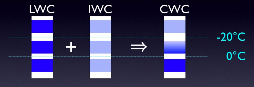
tion 2.2.4). The goodness-of-fit statistic is likewise identical.4 ALGORITHM THEORETICAL BASIS—CLOUD WATER CONTENT 17 Figure 1: The CWC composite profile is built by combining the retrieved ice and liquid water profiles, according to temperature. 4 Algorithm Theoretical Basis—Cloud Water Content The original list of CloudSat standard data products included separate products for liquid water content and ice water content. Because there was no independent means of determining the cloud phase in any given radar resolution bin, the plan was to run the liquid and ice retrievals separately on the entire radar profile, resulting in a set of liquid microphysical parameters for each cloudy bin and a corresponding set of ice microphysical parameters for each cloudy bin. The user would then select which answer would be more appropriate or combine the two in some way. No attempt would be made to partition the measured reflectivity between the liquid and ice phases—each solution would assume the entire radar signal was due to a single phase of water. As the retrievals were further developed and the time approached for the first post-launch data releases, it became clear that this approach would be overly confusing and would likely result in “double-counting” of the cloud water content: users interpreting each cloudy bin as containing both liquid and ice water content. To avoid this confusion, a new combined cloud water content product and algorithm were developed. In the new algorithm, the liquid and ice retrievals are run separately on the entire radar profile (as before), but the two resultant profiles are then combined into a composite profile using a simple scheme based on temperature. In this scheme, the portion of the profile colder than −20◦ C is deemed pure ice, so the ice retrieval solution applies there. Similarly, the portion of the profile warmer than 0◦ C is considered pure liquid, so the liquid solution applies there. In between these temperatures, the ice and liquid solutions are scaled linearly with temperature (by adjusting the ice and liquid particle number concentrations) to obtain a profile that smoothly transitions from all ice at −20◦ C to all liquid at 0◦ C while matching the radar measurements over the whole range. This scheme gives a very basic partition of the radar measurements into ice and liquid phases. (More sophisticated retrievals for heterogeneous cloud columns are planned for future versions of this product.) The product also contains a 16-bit status variable; individual bits in this variable indicate error conditions in the ice and liquid retrievals and other associated conditions such as large values of the fit parameters or possible precipitation. It is important to note that the partition algorithm is applied separately to the ice and liquid phases regardless of whether both retrievals were successful. For example, if the liquid retrieval fails to converge, the ice water content will still be scaled such that
4   ALGORITHM THEORETICAL BASIS—CLOUD WATER CONTENT                                                   18

it goes to zero as the temperature increases to 0◦ C—there is no attempt to map all the reflectivity to
the ice phase to compensate for the failure of the liquid retrieval.
    The 2B-CWC-RO data product files contain both the composite profiles (which most users will want
to use) and the single-phase retrieval profiles (which may be of interest to some investigators). The
output data from the liquid cloud retrieval (which interprets all cloud as liquid from the surface to the
stratosphere) is found in fields with names starting with LO_RO_ (for “liquid-only” and “radar-only”).
Corresponding outputs from the ice cloud retrieval have names starting with IO_RO_. The fields
representing the combination of these into composite profiles have names beginning with RO_liq_
and RO_ice_. Consult the 2B-CWC-RO Interface Control Document for detailed descriptions of the
fields contained in the 2B-CWC-RO HDF files.
5 ALGORITHM INPUTS 19 5 Algorithm Inputs 5.1 CloudSat 5.1.1 CloudSat 2B-GEOPROF Data The CloudSat 2B-GEOPROF product is the principal input for 2B-CWC-RO. The retrieval uses the radar reflectivity, the cloud mask, and the gaseous attenuation values from this product. For cases where this input is missing, 2B-CWC-RO will have no output. 5.1.2 CloudSat 2B-CLDCLASS Data Various bits in cloud scenario field in the 2B-CLDCLASS product are used to detect cloud type and to screen problematic profiles. Future versions of the retrievals may use the indicated cloud type, surface type, and other flags to refine the retrieval algorithm, for example by selecting different a priori values according to cloud type. 5.2 Ancillary (Non-CloudSat) 5.2.1 CloudSat ECMWF-AUX Data The retrieval uses temperature information from the CloudSat ECMWF-AUX product, which takes model output from ECMWF and interpolates the variables to the CloudSat data grid. Temperature information is used to assign a priori values in the ice cloud retrieval and also to guide the combination of the ice and liquid information into composite profiles.
6   ALGORITHM SUMMARY                                                                          20

6   Algorithm Summary
The algorithm is implemented in Fortran 90. The following is a pseudocode description of the algo-
rithm implementation:
start 2B-LWC-RO
get orbit of 2B-GEOPROF data (CPR cloud mask, radar reflectivity)
get orbit of 2B-CLDCLASS data (cloud scenario)
for-each 2B-GEOPROF vertical profile
     convert bit flags to integer values
     determine if LWC retrieval will be run (known & valid cloud scenario, cloud present, Z physi-
          cal)
     if running LWC retrieval
            determine size of state vector
            assign a priori rg , NT , and σlog values and uncertainties
            set y vector (2B-GEOPROF) using condensed profile retaining cloudy bins only
            set Sa , S−1
                       a , S matrices
            repeat
                calculate K, Sy , Dy matrices
                calculate F (forward-model) vector
                calculate S−1      −1
                              y , Sx , Sx matrices
                calculate new state vector x̂
                if x̂ goes negative, reject
                calculate ∆x̂, convergence test
                if more than 15 iterations, reject
            end-repeat until convergetest < 0.01n
            calculate re , LWC, LWP
            calculate χ2 and A
            calculate retrieval uncertainties
            calculate output percent uncertainties
            load output variables
     else
            ; RO LWC retrieval not run
            load output variables with error values and set status flags
     end-if (running LWC retrieval)
end-for (loop over profiles)
6 ALGORITHM SUMMARY 21
calculate metadata statistics
end 2B-LWC-RO
start 2B-IWC-RO
get orbit of 2B-GEOPROF data (CPR cloud mask, radar reflectivity)
get orbit of 2B-CLDCLASS data (cloud scenario)
for-each 2B-GEOPROF vertical profile
convert bit flags to integer values
determine if IWC retrieval will be run (known & valid cloud scenario, cloud present, Z physical)
if running IWC retrieval
determine size of state vector
assign a priori Dg , NT , and σlog values and uncertainties
set y vector (2B-GEOPROF) using condensed profile retaining cloudy bins only
set Sa , S−1
a , S matrices
repeat
calculate K, Sy , Dy matrices
calculate F (forward-model) vector
calculate S−1 −1
y , Sx , Sx matrices
calculate new state vector x̂
calculate ∆x̂, convergence test
if more than 15 iterations, reject
end-repeat until convergetest < 0.01n
calculate re , IWC, IWP
calculate χ2 and A
calculate retrieval uncertainties
calculate output percent uncertainties
load output variables
else
; RO IWC retrieval not run
load output variables with error values and set status flags
end-if (running IWC retrieval)
end-for (loop over profiles)
calculate metadata statistics
end 2B-IWC-RO6 ALGORITHM SUMMARY 22 start 2B-CWC-RO get orbit of 2B-GEOPROF data get orbit of 2B-LWC-RO data get orbit of 2B-IWC-RO data get orbit of ECMWF-AUX data calculate ice phase fraction from temperature for all cloudy bins calculate liquid phase fraction from temperature for all cloudy bins map liquid properties into composite profiles, scaling bins by liquid phase fraction map ice properties into composite profiles, scaling bins by ice phase fraction calculate revised ice and liquid water path from composite profiles copy error fill values into composite profiles add error codes for other error conditions set flags in status variable write metadata statistics to text file end 2B-CWC-RO
7   DATA PRODUCT OUTPUT FORMAT                                                                      23

7    Data Product Output Format
The 2B-CWC-RO data product includes swath data and metadata in an HDF-EOS formatted file.
Users are directed to the 2B-CWC-RO Interface Control Document for a full description of the data
and metadata fields contained in the product. Scale factors used in converting file values into science
data values are included in the file as HDF variable attributes. Users are encouraged to read scale
factors directly from the file (rather than from written documentation), because the scale factors may
change.

8    Changes since version 5.0
The following list summarizes the changes since version 5.0 of the 2B-CWC-RO product (which was
released in release R03):

    • Liquid Water Content
        – Number concentration and width parameter now allowed to vary with altitude
        – Change scale factor of some HDF variables
    • Ice Water Content
        – Change from modified gamma to lognormal size distribution
        – Number concentration and width parameter now allowed to vary with altitude
        – Change scale factor of some HDF variables
        – Change to temperature-based selection of a priori values
        – Omit cloudy bins warmer than +1◦ C (because no a priori values apply)
        – Change parameterization of fMie ratio
    • Cloud Water Content
        – Report profiles of all three size distribution parameters for both ice and liquid
        – Ice retrieval now uses lognormal distribution
        – Change scale factor of some HDF variables
REFERENCES 24
References
[1] Austin, R. T., and G. L. Stephens, Retrieval of stratus cloud microphysical parameters using
millimeter-wave radar and visible optical depth in preparation for CloudSat, 1. Algorithm formu-
lation, J. Geophys. Res., 106, 28 233–28 242, 2001.
[2] Austin, R. T., and G. L. Stephens, Improved retrieval of stratus cloud microphysical parameters
using millimeter-wave radar and visible optical depth, 1. Algorithm and synthetic analysis, in
preparation, 200X.
[3] Austin, R. T., et al., Improved retrieval of cirrus cloud microphysical parameters, in preparation,
200X.
[4] Benedetti, A., G. L. Stephens, and J. M. Haynes, Ice cloud microphysical parameters using mil-
limeter radar and visible optical depth using an estimation theory approach, J. Geophys. Res.,
108, 4335, doi:10.1029/2002JD002693, 2003.
[5] Bohren, C., and D. R. Huffman, Absorption and scattering of light by small particles, John Wiley
& Sons, Inc., New York, 1983.
[6] Fujita, M., and M. Satake, Rainfall rate profiling with attenuating-frequency radar using non-
linear LMS technique under a constraint on path-integrated rainfall rate, Int. J. Remote Sensing,
18, 1137–1147, 1997.
[7] Liu, C.-L., and A. J. Illingworth, Toward more accurate retrievals of ice water content from radar
measurements of clouds, J. Appl. Meteor., 39, 1130–1146, 2000.
[8] Marks, C. J., and C. D. Rodgers, A retrieval method for atmospheric composition from limb
emission measurements, J. Geophys. Res., 98, 14,939–14,953, 1993.
[9] Matrosov, S. Y., Retrievals of vertical profiles of ice cloud microphysics from radar and IR mea-
surements using tuned regressions between reflectivity and cloud parameters, J. Geophys. Res.,
104, 16 741–16 753, 1999.
[10] Miles, N. L., J. Verlinde, and E. E. Clothiaux, Cloud droplet size distributions in low-level strati-
form clouds, J. Atmos. Sci., 57, 295–311, 2000.
[11] Rodgers, C. D., Retrieval of atmospheric temperature and composition from remote measure-
ments of thermal radiation, Rev. Geophys., 14, 609–624, 1976.
[12] Rodgers, C. D., Characterization and error analysis of profiles retrieved from remote sounding
measurements, J. Geophys. Res., 95, 5587–5595, 1990.
[13] Rodgers, C. D., Inverse Methods for Atmospheric Sounding: Theory and Practice, World Scien-
tific Publishing, Singapore, 2000.
[14] Stephens, G. L., Remote sensing of the lower atmosphere, Oxford University Press, Oxford, 1994.You can also read