Life history and population dynamics of southern Alaska resident killer whales (Orcinus orca)
←
→
Page content transcription
If your browser does not render page correctly, please read the page content below
MARINE MAMMAL SCIENCE, 30(2): 460–479 (April 2014)
© 2013 Society for Marine Mammalogy
DOI: 10.1111/mms.12049

  Life history and population dynamics of southern Alaska
              resident killer whales (Orcinus orca)

CRAIG O. MATKIN,1 North Gulf Oceanic Society, Homer, Alaska 99603, U.S.A.; J. WARD
TESTA, Alaska Fisheries Science Center, 7600 Sand Pt. Way, NE, Seattle, Washington
98115, U.S.A. and Department of Biological Sciences, University of Alaska Anchorage,
Anchorage, Alaska 99508, U.S.A.; GRAEME M. ELLIS, Department of Fisheries and Oceans,
Pacific Biological Station, Nanaimo, British Columbia V6T 6N7, Canada; EVA L. SAULITIS,
North Gulf Oceanic Society, Homer, Alaska 99603, U.S.A.

                                           Abstract
         Resident (fish eating) killer whales (Orcinus orca) in the North Pacific have been
      the subject of long-term studies in several geographical regions. The current study
      examines population parameters in the southern Alaska resident population from
      1984 to 2010 and develops a population model. The southern Alaska resident
      population ranges from southeastern Alaska through the Kodiak archipelago and
      contains over 700 individuals. We follow the life histories of 343 identifiable whales
      in 10 pods from two clans born before and during the study. Population parameters
      were comparable to those of the British Columbia northern resident population dur-
      ing the 1970s and 1980s, except that age of maturity was approximately one year
      earlier. The average annual rate of increase was slightly higher in Alaska (3.5%) than
      for the British Columbia northern residents (2.9%) and probably represents a popu-
      lation at r-max (maximum rate of growth). Reasons for the high growth rate in
      Alaska could be a recovery following past anthropogenic mortalities, or more likely,
      a response to increasing salmon returns in recent decades, resulting in an increase in
      carrying capacity. The slow maturation and low rate of reproductive response makes
      these whales slow to recover from natural or anthropogenic catastrophes.

      Key words: killer whales, Orcinus orca, population dynamics, southern Alaska, life
      history, residents.

   Killer whales have a cosmopolitan distribution and are top-level predators.
Studies in the eastern North Pacific indicate that at least three ecotypes exist in
this region: residents, transients, and offshores (Matkin et al. 1999a, Ford et al.
2000). Despite their sympatric distribution, these ecotypes do not associate or
interbreed and are acoustically and genetically distinct (Hoelzel and Dover 1991;
Hoelzel et al. 1998, 2007; Barrett-Lennard 2000; Yurk et al. 2002).
   The resident ecotype preys almost exclusively on fishes (Ford et al. 1998, Saulitis
et al. 2000) and has been studied along the length of the eastern North Pacific coast
from California to the Aleutian Islands and the southern Bering Sea (Matkin et al.
1999a, Ford et al. 2000, Matkin et al. 2007). It has been separated by genetic analysis,
  1
   Corresponding author (e-mail: comatkin@gmail.com).

                                              460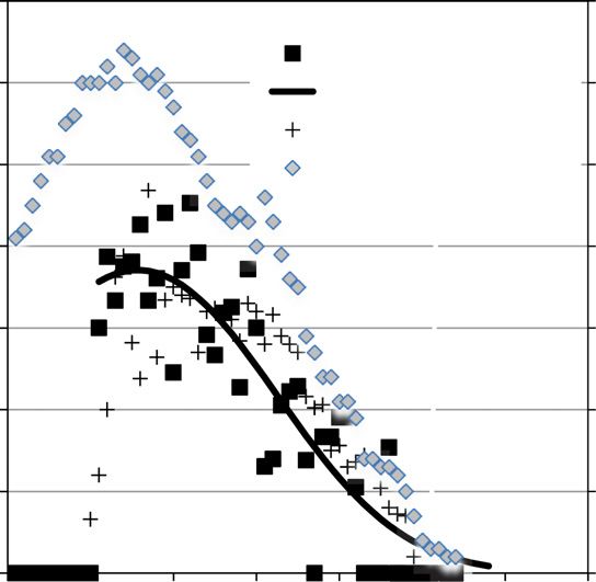
MATKIN ET AL.: KILLER WHALES                               461

acoustics, and association into three populations (Matkin et al. 1999a, Barrett-Lennard
2000, Ford et al. 2000, Yurk et al. 2002, Allen and Angliss 2010). The southern resi-
dent population has been the subject of studies centered in Puget Sound and Washing-
ton State waters since the late 1970s (Balcomb et al. 1982, Bigg et al. 1990, Olesiuk
et al. 1990, Ford et al. 2000) and has been listed as endangered under the U.S. Endan-
gered Species Act and the Canadian Species at Risk Act. The British Columbia north-
ern resident population is listed as threatened in Canada and is encountered primarily
in the waters of British Columbia although they range into southeastern Alaskan
waters where there is overlap with at least two pods in this study (Bigg 1982, Bigg
et al. 1990, Ford et al. 2000). A third population, the southern Alaska residents,
ranges from southeastern Alaska at least as far west as the Kodiak archipelago (Matkin
et al. 1999a, Allen and Angliss 2010). It is the subject of this analysis.
   Our analysis is possible because of unusual attributes of resident killer whales that
are not shared by the other ecotypes. They are relatively accessible with a high proba-
bility of encountering individuals on an annual basis, and they travel in maternal
groupings that change composition only as a result of births or deaths. These perma-
nent associations facilitate the repeated identification of individuals and allow accu-
rate annual tracking of individuals within maternal groups and for a substantial
segment of the population.
   The field and analytical techniques we use were first developed in long-term studies in
British Columbia and Washington State. Using direct observation, annual photographic
census, and statistical inference, Bigg et al. (1990) established genealogies and estimated
ages of individuals for the northern and southern resident populations of killer whales.
These techniques were later applied to the southern Alaska resident population by
Matkin et al. (1999a, b). Olesiuk et al. (1990) estimated life history parameters and
described population dynamics of northern and southern resident killer whales based on
the demographic changes observed from 1973 to 1987. More recently, Olesiuk et al.
(2005) used updated information to examine changes in population trajectory and to
develop a new population model for northern residents from 1973 to 2004.
   An understanding of the dynamics of killer whale populations provides insight
into how they function and respond to various impacts. For example, Olesiuk et al.
(1990) used their model to assess long-term impacts of a killer whale live-capture
fishery that had altered the sex- and age-structure of the populations in British
Columbia and Washington State. Later, Olesiuk et al. (2005) demonstrated possible
impacts of prey abundance on the population trajectory of the northern residents. We
used some earlier results from our work to examine the effects of the Exxon Valdez oil
spill (Matkin et al. 2008).
   In the current study, we modify methodologies originally developed by Olesiuk
et al. (2005) to describe life histories, develop population parameters, and construct a
population model for southern Alaskan resident killer whales. The study was based
on systematic long-term photo-identification surveys conducted annually from 1984
to 2010. Here, we detail the parameters of the model to describe a population increas-
ing at a rate approaching r-max but vulnerable to changes in environment or prey
populations.
                                       Methods
Study Area and Population
  The range of the southern Alaska resident pods described in this study includes the
northern Gulf of Alaska and inshore waters from southern southeastern Alaska
462 MARINE MAMMAL SCIENCE, VOL. 30, NO. 2, 2014 through the Kodiak archipelago (Matkin et al. 1999b, Fig. 1). Most pods appear to have a more limited range within this region (Matkin et al. 1997, Matkin et al. 1999a, Scheel et al. 2001) and the extent that these whales use waters south and west of Kodiak Island is unclear. Past and current studies in Alaska west of the Shumagin Islands have not identified individuals from the resident pods described here (Dahl- heim and Waite 1992, Dahlheim 1997, Matkin et al. 2007, Durban et al. 2010). Parsons et al. (in press) has determined genetic strata from nDNA analysis that sug- gest a population separation of resident type killer whales that occurs south of Kodiak Island. At the southeast end of their range, in southeastern Alaska, the southern Alaska residents have been observed in close proximity to members of the British Columbia northern resident population, but mixing between these groups has not been reported (Dahlheim et al. 1997, Barrett-Lennard 2000, Ford et al. 2000). A genetic separation of southern Alaska residents from the parapatric British Columbia northern residents was indicated by the examination of 11 microsatellite loci (Barrett-Lennard 2000), although there may be occasional matings between the groups. In contrast, observa- tion and analysis indicates that pods and individuals within the southern Alaska resi- dent population examined here regularly intermingle and interbreed (Matkin et al. 1997, Matkin et al. 1999b, Barrett-Lennard 2000). In our analyses the southern Alaska residents were considered as a single and sepa- rate population consisting of two sympatric, freely interbreeding acoustic clans that are separable by mtDNA haplotypes and by acoustic repertoire (Yurk et al. 2002). Within our study population, genetic evidence indicates successful breeding occurs primarily between individuals from the more distantly related pods within the clan Figure 1. Range of the southern Alaska resident killer whale population in the eastern North Pacific.
MATKIN ET AL.: KILLER WHALES                            463

(Barrett-Lennard 2000). Our analysis focuses on a subset of pods from both acoustic
clans that are most likely to be repeatedly encountered on an annual basis and whose
size ranges from 6 to 42 individuals. Our results describe only the dynamics of this
large subset of the population although it may reflect overall population characteris-
tics as suggested by Olesiuk et al. (1990).

Data Collection
   Our study required an annual census that was initiated in 1984 and continued
through 2010, though effort declined following 2005 and some pods were not seen
in all of the last five years. We annually attempted to photographically identify each
individual whale in the 10 pods that comprised our sample. We did not include the
well-described AB pod in our analysis due to the anomalous mortalities following the
Exxon Valdez oil spill reported elsewhere (Matkin et al. 2008). Data collection proce-
dures followed those described by Bigg et al. (1990) and Matkin et al. (1999b).
Although some fieldwork occurred in all months of the year, in all years the vast
majority of effort and encounters with killer whales occurred from early May through
October. Our data are considered annual surveys of the population that occurred dur-
ing the spring, summer, and fall period.
   The techniques used to approach and photograph the whales were consistent over
the duration of the study. Whales were approached from the left side or from behind
to a lateral distance of 15–30 m. Photographs were always taken of the left side of
each whale showing details of the dorsal fin and gray saddle patch. In the most useful
photographs the whale filled at least 50% of the frame. We attempted to obtain pho-
tographs of all whales in each encounter; however, this was not always possible due to
conditions of weather or light, and for larger groups it often required multiple
encounters to completely photograph all whales.
   Initially a 35 mm SLR Nikon FM2 camera with a manual focus 300 mm lens and
shoulder brace mount was used, but in the 1990s autofocus cameras were introduced
and for many years a Nikon F-100 camera with an autofocus 300 mm f:4.5 lens was
the preferred tool. In the early years Illford HP5 400 ASA black and white negative
film was used and push-processed to 1600 ASA; later Fuji Neopan 1600 proved to be
the most useful film. In recent years photographs have been acquired with Nikon
D-200 or D-700 digital cameras with a 300 mm autofocus lenses.

Individual Identification
   All film negatives collected during the fieldwork were examined under a Wild M5
or M8 stereomicroscope with 109 eyepieces. Digital images were examined using
PhotoMechanic software (Camera Bits Inc., Hillsboro, OR) on an Apple computer
with a 24 in. high resolution LCD screen. Identifiable individuals in each frame were
recorded. When identifications were not certain, they were not included in the analy-
sis. Reference files of 5 9 7 prints of each individual were replaced on an annual basis
if new marks, fin maturation or other changes necessitated an update. Each individual
was labeled based on an alphanumeric code developed at the beginning of the study
(Leatherwood et al. 1990) and used in sequential catalogs (Matkin et al. 1999a, b).
The first character in the code is “A” to designate Alaska, followed by a letter (A–Z)
indicating the individual’s pod. Individuals within the pod received sequential num-
bers. For example, AB03 is the third whale designated in the AB pod. New calves
were identified and labeled with the next available number. If a pod split, each new
464                     MARINE MAMMAL SCIENCE, VOL. 30, NO. 2, 2014

pod was designated after the alphanumeric code of a primary matriarch, but the
alphanumeric designation of individuals remained the same and new animals were
designated using the original alphabetic pod designation.
   Olesiuk et al. (1990) showed that the male fin of northern resident killer whales
could be statistically distinguished from that of females when it reached a height-to-
width ratio (HWR) of 1.4, which appears to occur during adolescence and
concurrently with development of other secondary sexual characteristics such as
enlargement of pectoral fins and the downturn of fluke tips. For males, we calculated
maturation statistics for the age at which HWR reached this threshold, and for the
age at which the dorsal fin reached its full height and males were judged to be
completely mature.

Age Estimation
   Following the approach developed by Bigg et al. (1990) and modified by Olesiuk
et al. (2005) for British Columbia and Washington State resident killer whales, we
used genealogies developed for southern Alaska resident killer whales (Matkin et al.
1999a, b) to establish ages. Killer whales used in this analysis were aged using the
following criteria:

(1) Animals born during or just prior to the study were aged on the basis of year first
    observed, which in most cases corresponded with year they were born (n = 187).
    Growth is rapid the first few years, facilitating age estimation up to about 3 yr
    from size (Olesiuk et al. 1990, 2005). Animals estimated from their size to be
    ≤3 yr old when first seen were assumed to be known-age (n = 42).
(2) Most older juvenile animals born prior to the study were aged based on the year
    they matured. However, for a few animals that died prior to maturation, birth
    year was estimated from size. Nine animals were aged in this group with a possi-
    ble aging error of 3 yr.
(3) Females that were juvenile-sized when first seen but larger than average 3 yr old
    whales were aged by subtracting mean age of first recruitment (13 yr), as esti-
    mated from known-age animals from the year they were seen with their first calf.
    Twenty-one females were aged using this calculation with a possible aging error
    of 2 yr.
(4) Forty females that were adult-sized when first seen were aged by subtracting
    mean age of first reproduction (AFR, 13 yr) from year of birth of their oldest
    known calf. We did not use a correction factor as in Olesiuk et al. (2005) to com-
    pensate for older calves that may have died before the beginning of the study (see
    Discussion).
(5) Males that were juveniles when first seen but too large to estimate based on size
    were aged by subtracting mean age of onset of sexual maturity (13) determined
    in this study (below). There were 22 whales aged in this manner with a potential
    error of –3 to +2 yr.
(6) Males that were sexually but not physically mature when first seen were aged by
    subtracting mean age of onset of physical maturity (18) determined in this study
    (below). Six whales were aged in this manner with a potential error of 3 yr.
(7) Males that were physically mature when first seen were aged on the basis of the
    year they were first seen by subtracting the average age of onset of physical matu-
    rity (18 yr). These were considered minimum ages. A total of 16 whales were
    aged in this manner.
MATKIN ET AL.: KILLER WHALES 465
Age of First Reproduction (AFR) and Reproductive Rates
We estimated the mean age at first reproduction using the method by DeMaster
(1978) based on the proportion of females and males mature at each age. For females,
we defined maturation as the age at which they began contributing to recruitment in
the population, which was the age at which we observed their first calf. Calving sea-
son apparently occurred during the November to April period, since most calves were
born prior to the annual census which was not initiated until early May, and few
calves were born during the May–October field season. We were essentially censusing
the recruitment of calves from 1 to 6 mo of age, not birth rate. No female less than
11 yr old was observed with a calf, so only females seen each year from age 11 until
the recruitment of their first calf were included in the analysis. Known-age females
excluded from calculations of mean age at first reproduction due to a missing observa-
tion were reincluded in the analysis of other population parameters.
In calculating variance, DeMaster’s (1978) method assumes that observations at
each age are independent, which cannot be justified in longitudinal samples such as
those obtained here (or by Olesiuk et al. 1990, 2005). We therefore used bootstrap
sampling (Efron 1982) of individual whale sighting histories to estimate variances
and confidence intervals around mean age of sexual maturity. A bias exists in this
estimator as applied by Olesiuk et al. (1990, 2005) in that the sex of most juveniles
is not determined until sexual maturity is reached, and some whales disappeared
before their sex was known. This introduces a negative bias due to exclusion of some
immature animals and overestimation of the proportion mature at a given age. We
present estimates without correction for this bias in order to compare to results of
Olesiuk et al. (2005), as well as estimates in which we include juveniles of unknown
sex in our bootstrap sampling with an additional bootstrap assignment of sex from an
even sex distribution to exclude approximately half of the unknown sample. This
method still retains some bias due to the small difference in age at maturity of the
two sexes, which creates a slight underestimate of age at maturity in females and an
overestimate for males. This correction was not needed for male age at full maturity
because of the long physical maturation period for males as evidenced by the gradual
growth of the dorsal fin. The sex was known for all males used in that calculation well
before the youngest age for full maturity had been reached. In all cases, the bootstrap
median was closer to the direct calculation of mean age of maturity (DeMaster 1978)
than the bootstrap mean, and we report only the median estimate.
We established one measure of female fecundity by estimating the intervals
between successive calves and determining the probability of calving in a given year:
FEC ¼ 1=CI;
where FEC is the proportion of females giving birth each year and CI is the interval
between successive calves. For instance, if females gave birth once every five years, the
probability of giving birth in any given year is 0.2. We used bootstrap sampling (Efron
1982) of individual calving records to determine the median and confidence interval.
Age-specific fecundity rates of females FECf(x) was defined as the proportion of
females aged x giving birth to viable calves each year:
FECf ðxÞ ¼ NCf ðxÞ=Nf ðxÞ;
where NCf(x) denotes the number of calves of either sex born to females aged x, and
Nf(x) the total number of females aged x. We used all females, but inclusion of466 MARINE MAMMAL SCIENCE, VOL. 30, NO. 2, 2014
females aged by the birth of their first calf would have caused a spurious spike of
births at age 13. We therefore distributed those births normally around the most
unbiased estimated age of first successful reproduction (AFR) as calculated above for
purposes of smoothing the age-specific rates around the AFR. There are gaps in the
resighting records in which calving events are reconstructed from mother-offspring
associations discovered when the pods were resighted and these have a potential to
create a small but off-setting bias to adult reproductive rates and calf survival. With
the very high survival rates observed here, the potential bias is small. We used a sec-
ond order polynomial logit model in the R statistical package glm (R Development
Core Team 2010) to smooth the age-specific reproductive curve beginning at age 11,
the earliest observed age for a first surviving calf.
Mortality and Survival Rates
Mortality and survival rates were estimated by monitoring individuals over time.
In 36 yr of monitoring resident whales in British Columbia and Washington, and
26 yr in Alaska, there is no evidence of dispersal from matrilines (Bigg et al. 1990,
Matkin et al. 1999a, Olesiuk et al. 2005, Matkin et al. 2008). Animals that disap-
peared were thus assumed to have died. Rates were estimated as:
MRðxÞ ¼ 1 SRðxÞ ¼ DðxÞ=NðxÞ;
where MR(x) represents the annual mortality rate or probability of dying in the next
year at age x, SR(x) the annual survival rate or probability of surviving the next year
at age x, D(x) the number of animals aged x that died before reaching age x + 1, and
N(x) the number of animals in the study population aged x that were monitored to
age x + 1. Where year of death was uncertain, we amortized the death over the
2–3 yr of uncertainty in the manner of Olesiuk et al. (2005).
Because mortality and survival often changes most rapidly early in life, and to take
advantage of larger samples sizes for younger age groups, we pooled data into pro-
gressively wider age categories: 0.5–1.5 yr, 1.5–2.5 yr, 3.5–5.5 yr, 6.5–9.5 yr, and
10.5–14.5 yr, which are the same categories used by Olesiuk et al. (1990, 2005).
New calves were assumed to be approximately 0.5 yr of age since most births occur
in winter and recruited calves are not observed until months later. Animals that were
not seen as calves, but later aged by their size or apparent maturity, were excluded
from analyses in the first year of sighting because of the positive bias created in sur-
vival to that age. The effect of uncertainty in the ages of larger juveniles was negligi-
ble due to the pooling of the older categories. Standard errors and confidence
intervals of the estimates were calculated by bootstrap sampling of individuals (Efron
1982). To account for decreasing sample sizes and increasing imprecision in age esti-
mates with age, we pooled observations in 5 or 10 yr increments for the oldest age
classes. Since we do not know the maximum ages with certainty, the older classes
may encompass a larger range than indicated.
Population Model
As a heuristic tool a population model was constructed for comparison with the
observed population dynamics and those of the northern resident population. Esti-
mated age-specific survival and birth rates were applied to the starting population
age/sex structure in 1984 and projected forward until a constant growth rate andMATKIN ET AL.: KILLER WHALES 467
stable structure was reached. This was verified by life table analysis using Lotka’s fun-
damental equation (Lotka 1907, Olesiuk et al. 2005). The survival and birth sched-
ules for the northern resident killer whale population studied by Olesiuk et al.
(2005) was also modeled, duplicating the model described by those authors but
allowing direct comparison of our results without ambiguity that might arise from
rounding-off and other discrepancies in demographic estimates. Since we were uncer-
tain of maximum ages in our study, we allowed the same maximum ages (age 90 for
females and age 70 for males) in our model as did Olesiuk et al. (2005). In practice,
truncation at age 60 for females and age 40 for males had negligible effect on age
structure. Population growth (k) is defined as the quotient of total population size in
successive years (Nt/Nt–1), either from observations or as modeled. Applying the pop-
ulation model to the starting age/sex structure in the population allowed a compari-
son of population growth and structure which should have occurred if vital rates were
constant as estimated over the study to those actually observed.
Our modeling efforts were, in part, intended to confirm the validity of our vital
rate estimates, but also to explore the implications of subtle differences that might be
seen in between our observed and modeled growth and age structure, and between
our results and those of Olesiuk et al. (2005) for the northern resident killer whales
of British Columbia. We used the survival data in Table 2 and the polynomial
regression of calving rates in Figure 4 to estimate population growth and age/sex
structure from the observed population size and age/sex composition in 1984. We
used the most precise estimates of survival and calving rates available from Olesiuk
et al. (2005: table 7, 8 for survival and table 10 for fecundity) for the northern resi-
dent killer whale population during its period of exponential growth (1973–1996) to
recreate their life table model and standardize comparisons between the two popula-
tions. The “postreproductive” class in both studies is somewhat problematic because
the reproductive criterion (no calves in last 10 yr) used by Olesiuk et al. (1990,
2005) is of limited utility at the end of a study lasting only 20 or 30 yr, and because
the gradual decline in reproduction with age (Fig. 4 and Olesiuk et al. 2005: fig. 15)
makes such determination ambiguous. We have used the “average age of senescence”
of 40.5 yr (Olesiuk et al. 2005) as a general cut-off between reproductive and postre-
productive classes in our analysis.
Results
We have identified over 700 whales in the southern Alaska resident population
during this study. However, we were able to regularly locate and reidentify only 343
of these whales, which composed 10 pods. There were four pods from the AD clan
(AD05, AD16, AE, and AK) and six from the AB clan (AF05, AF22, AG, AI, AJ,
and AN10). We excluded two other pods (AB and AB25) that experienced atypical
mortalities following the Exxon Valdez oil spill (Matkin et al. 2008). These 10 study
pods and the number of whales in each are presented in Table 1.
All individuals from all of our monitored pods were not photographed in every
year with one year intervals between documentation occurring 8% of the time, two
year intervals 2% of the time and three year intervals 1% of the time (Table 2).
The number of whales in 10 pods that were seen from 1984 to 2005 increased from
121 whales to 240 at a mean annual growth rate of 3.4%. The seven pods seen from
1984 to 2010 increased from 82 to 152 at a mean annual rate of 2.6% (Fig. 2).
Because 3 of the pods (AF05, AF22, AG) in southeastern Alaska (Matkin et al. 1997,468 MARINE MAMMAL SCIENCE, VOL. 30, NO. 2, 2014
Table 1. Recruitment, mortalities, and total number of whales by pod, 1984–2010, with
exceptions of AF05 and AF22 (last counted in 2005), and AG, (last counted in 2008).
Total Total Total
Pod 1984 recruited died Total
AD05 13 16 10 19
AD16 6 8 6 8
AE 13 13 9 17
AF05 12 32 6 38
AF22 12 25 9 28
AG 15 30 6 39
AI 6 4 3 7
AJ 25 42 12 55
AK 7 15 7 15
AN10 12 29 10 31
Total 121 182 78 264
1999a) were usually out of our study area, they could not be tracked consistently
between 2005 and 2010 and our examination of population characteristics is based
on the 1984–2005 data from all pods. The difference in growth rates (Fig. 2) is at
least partly explained by a female-skewed adult sex ratio in these three large pods that
were not observed consistently in the final years. It is likely that the inter-pod vari-
ance in growth rate also is due to variance in adult reproductive output based on indi-
vidual life histories (Brault and Caswell 1993).
Life History Parameters
Thirty-eight known-age females >10 yr of age were initially considered for
analysis of AFR, but seven were excluded because of gaps in their sighting history
in the period when they were 11–15 yr of age, the age range at which first calves
were observed among females without resighting gaps. Excluding the nine juve-
niles of unknown sex led to a calculated mean (after DeMaster 1978) AFR of 12.8
(SE = 0.15), and a bootstrap median AFR of 13.1 (bootstrap 95% CI = 12.6–13.7,
SE = 1.40). Median AFR including nine unsexed juveniles was 13.3 (bootstrap 95%
CI = 12.7–13.8, SE = 1.18; Fig. 3). Among known-age females observed with a first
calf, the modal AFR was 12 yr, indicating a positive skew in the distribution of
AFR.
At an age range of 10–16 yr, the fins of a total of 44 known-aged males were esti-
mated to have attained a height to width ratio (HWR) of 1.4, which is the ratio that
marked the onset of sexual maturation developed by Olesiuk et al. (1990) in British
Columbia. The estimated mean age at onset of sexual maturation (after DeMaster
1978), excluding juveniles of unknown sex, was 12.4 (SE = 0.14). The bootstrap
median age at onset of sexual maturation of that sample was 12.4 yr (bootstrap 95%
CI = 12.0–12.9, SE = 1.12); for the sample including unsexed juveniles (n = 53) the
median was 12.5 yr (bootstrap 95% CI 12.1–13.0, SE = 1.01; Fig. 3).
At the age range of 15–21 yr, 22 known-age males reached physical maturity dur-
ing the study as indicated by a fully developed dorsal fin. Direct calculation of the
average age of full maturity (after DeMaster 1978) from 36 known-age males ≥15 yr
of age produced an estimate of 18.3 yr (SE = 0.19). Bootstrap median age of full
maturity was 18.3 (bootstrap 95% CI = 17.6–19.0, SE = 1.45; Fig. 3).MATKIN ET AL.: KILLER WHALES 469
Table 2. Intervals between annual photodocumentation of individuals within each pod
from 1984 to 2005 with proportion of total in parentheses (n = 3,610).
Pod 0 yr 1 yr 2 yr 3 yr 4 yr 5 yr
AD05 281 15 4 6 2 1
AD16 118 9 5 2 0 0
AE 227 26 2 1 0 0
AF05 353 29 22 5 1 0
AF22 353 61 25 3 0 0
AG 469 46 14 2 0 0
AI 141 0 0 0 0 0
AJ 668 53 10 0 0 0
AK 228 8 0 0 0 0
AN10 388 32 0 0 0 0
Total 3,227 (0.89) 279 (0.08) 82 (0.02) 19 (0.01) 3 1
250
200
ln(N)=0.034y-62.90
150
Population Size
100
ln(N)=0.026y - 47.38 All
Pods
50
7 Pods
0
1980 1990 2000 2010
Figure 2. Population trend for 10 pods of southern Alaska resident killer whales from 1984
to 2005 (top) and for seven of those pods that were monitored through 2010.
We documented the intervals between births of 198 viable calves of 59 females for
which at least two births were recorded (139 intervals). Calves were produced at
intervals of 2–14 yr (Fig. 4), but most were separated by 3–7 yr (mean 4.9,
bootstrap median = 4.8, SE 0.63, 95% CI = 4.4–5.2). The bootstrap median annual
calving rate (FEC) among these reproductive females was 0.21 (SE = 0.01, 95% CI =
0.19–0.23).
There was little evidence that calving intervals changed over the period of the
study (regression slope = 0.05, P = 0.15). Mean calving intervals increased signifi-
cantly (regression slope = 0.22, P < 0.01) with age of the mother, from 4.3 yr at age
20 to about 6.5 yr by age 40. The number of calves produced by each individual per
year declined with age (Fig. 5) due to the longer calving intervals and apparent onset
of senescence. This pattern was also observed in the northern resident killer whale470 MARINE MAMMAL SCIENCE, VOL. 30, NO. 2, 2014
1.0
0.8
0.6
Proportion Mature
0.4
Female First Calf
0.2 Male Onset
Male Full Maturity
0.0
8 10 12 14 16 18 20 22
Age (yr)
Figure 3. Age of sexual maturity (first calf) in known-age females and males (onset of dorsal
fin growth) and male full maturity as judged by dorsal fin development for southern Alaska
resident killer whales.
population in British Columbia (Olesiuk et al. 2005) and in the short-finned pilot
whale (Globicephala macrorhynchus) (Marsh and Kasuya 1986).
Survivorship for both males and females conformed to the classic mammalian
U-shaped curve (Table 3), indicating that the youngest and oldest animals experi-
enced the highest mortality; however, the curve was narrower for males than females
with a significant increase in mortality for males in the 30–41 yr range and for
females in the 50–54 yr range, indicating a longer lifespan for females. Mortality
rates for juveniles could not be estimated separately for each sex because deaths of
immature animals (as old as 15 yr) could not be accurately assigned to sex. For this
reason, and to facilitate comparison to northern resident killer whales, survival rates
were estimated for both sexes pooled up to the age of 15.5 yr, as per Olesiuk et al.
(2005).
Population Dynamics
While the average annual population growth rate (k) of all pods from 1984
to 2005 was 1.035 (e0.0341; Fig. 2), the initial modeled growth declined during
the course of the study, and converged to 1.024 at stable age distribution. How-
ever, the sex ratio of whales observed as juveniles and reaching the age of
15.5 yr was skewed toward females (55:45). While not a statistically significant
deviation from an even sex ratio (P = 0.18), in this study, where all individuals
are tracked, it creates observed effects on population growth. It is not known
whether the skewed sex ratio was present at birth or the result of differences in
neonatal and juvenile mortality up to maturity. To compensate we modified our
model by creating a 55:45 female to male ratio which elevated the modeled
growth rate from 1999 to 2005 slightly (1.026 vs. 1.024 in 2005), and gave a
growth rate of 1.029 when stable age structure is achieved (Fig. 6). Mean annual
growth rate and number of deaths in the modeled population were identical toMATKIN ET AL.: KILLER WHALES 471
40
35
Frequency 30
25
20
15
10
5
0
1 2 3 4 5 6 7 8 9 10 11 12 13 14
Calving interval (yr)
Figure 4. Frequency distribution of calving intervals for southern Alaska resident killer
whales.
0.35 70
SAR Calving rate
0.30 SAR model 60
NR Calving rate
0.25 Sample size NR + SAR 50
Proportion Calving
Number of Females
0.20 40
0.15 30
0.10 20
0.05 10
0.00 0
0 10 20 30 40 50 60 70
Age (yr)
Figure 5. Age-specific fecundity (calves/female) for both southern Alaska resident (SAR)
and northern resident (NR) and sample sizes for all females (both populations). Sample shown
includes 21 SAR females that were first observed as juveniles and aged by the year in which
they were first seen with a calf; these were distributed normally around the estimated age of
first reproduction (13.3 yr) from ages 11 to 16. Model for SAR was a 3rd order logit polyno-
mial fit to ages 11–52.472 MARINE MAMMAL SCIENCE, VOL. 30, NO. 2, 2014
Table 3. Age and sex-specific annual survival rates from bootstrap analysis of southern
Alaska resident killer whales.
Age class n Upper 95% Median survival Lower 95% Mean SE
Both sexes
0–1.5 165 0.976 0.945 0.903 0.946 0.019
1.5–2.5 181 1.000 0.997 0.991 0.997 0.003
3.5–5.5 179 0.998 0.991 0.981 0.990 0.004
6.5–9.5 163 0.996 0.989 0.979 0.988 0.005
10.5–14.5 141 0.998 0.992 0.983 0.992 0.004
Females
15–19 63 1.000 0.996 0.988 0.996 0.004
20–24 56 1.000 0.987 0.970 0.987 0.008
25–29 44 1.000 0.990 0.973 0.989 0.007
30–34 43 0.984 0.960 0.924 0.959 0.016
35–39 27 0.992 0.968 0.932 0.968 0.016
40–50 19 0.989 0.958 0.922 0.958 0.016
50–54 4 1.000 0.800 0.500 0.783 0.146
Males
15–19 66 0.998 0.986 0.967 0.985 0.008
20–24 47 0.985 0.964 0.933 0.962 0.014
25–29 32 0.993 0.965 0.932 0.964 0.015
30–34 20 1.000 0.970 0.921 0.966 0.020
35–41 11 0.945 0.857 0.731 0.854 0.054
those observed (1.033 and 69, respectively), while calf production differed by 1
(190 vs. 191).
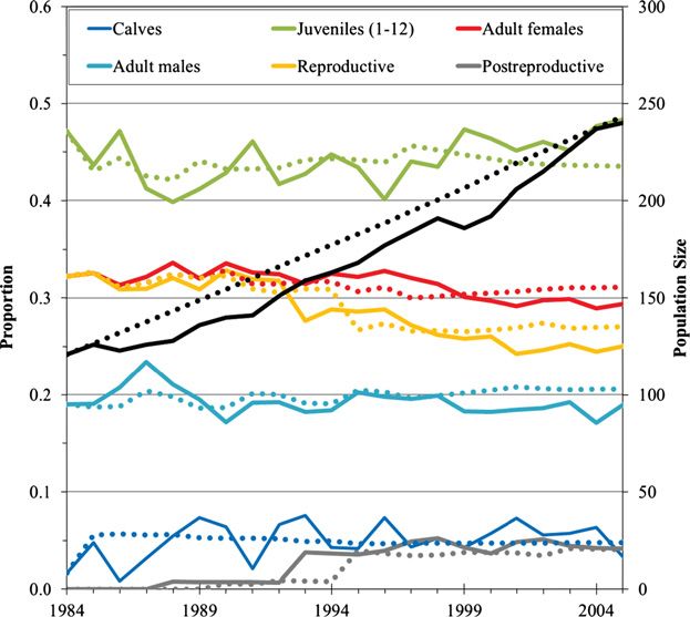
The observed rate of population growth lagged the model growth early in the
study (Fig. 6) with somewhat higher than average rates of calving and juvenile
recruitment in the final six years (Fig. 7). The decline in modeled growth rate
(Fig. 6) is the result of a higher proportion of adult, particularly reproductive,
females at the start of the study in comparison to a stable distribution, but the
increased calf and juvenile recruitment after 1999 appears to have increased the juve-
nile proportion relative to earlier in the study, and brought it up to a higher propor-
tion than predicted by the model at stability (Fig. 7).
There are some minor artifacts in the model that largely stem from the averaging
of estimated demographic parameters. The shift in reproductive and postreproductive
females beginning in 1993 (Fig.7) is likely an artifact of underestimating the age of
females that should have been in the postreproductive class at the beginning of the
study, and this may be responsible for the model overestimating population growth
in the early years of the model, and underestimating growth later due to having
underestimated fecundity. There were eight females that were classified as postrepro-
ductive in 1984 by the criterion that they produced no offspring in the next 10 yr,
but their ages were likely underestimated by a conservative age determination refer-
enced to the likely age of their oldest known offspring. If those animals (estimated
ages 18–36 yr, mode = 31) were distributed across the 40–55-yr-old ages, the mod-
eled population growth would have declined to ~1.034 at the beginning of the study
instead of 1.043 (Fig. 6).
The rates and stable age/sex structure of the model developed for southern Alaska
resident killer whales is very similar to that of northern resident killer whales in their
period of unrestrained population growth (Olesiuk et al. 2005) (Table 4).MATKIN ET AL.: KILLER WHALES 473
Figure 6. Observed and modeled rates of annual population growth of resident killer
whales, demonstrating a weak positive trend from the observations. Model estimates were
based on estimated average rates of survival and calving applied to the starting age/sex struc-
ture of killer whales in 1984, and an observed skew toward females (55:45) in newly matured
whales.
Vital rates in our study produced slightly more reproductive females and juveniles,
and slightly fewer males and fewer postreproductive females. Expected lifetime
production of calves was slightly higher in the northern residents, but stable popula-
tion growth was essentially equal. The evidence for a difference is strongest in age of
maturity, where southern Alaska residents of both sexes were estimated to mature
roughly a year earlier than those of Olesiuk et al. (2005). However, the bootstrap var-
iation was substantially higher, and our inclusion of unsexed juveniles lead to higher
estimates such that there was virtually complete overlap in the estimates of all age-
specific parameters from the two populations (see Fig. 5 and Table 3). In both stud-
ies it is likely that some bias occurs in prime-age survival and reproductive rates as a
result of underestimating the ages of mature females at the beginning of the study,
but the exercise of distributing some of these to later ages indicated that the numbers
and bias are probably small.
Discussion
Although the two populations are genetically distinct (Barrett-Lennard 2000,
Matkin et al. 1999a), the population biology of the southern Alaska residents was
remarkably similar to that of the northern residents of British Columbia during the
1970s through early 1990s when that population was increasing at 2.9% annually
(Olesiuk et al. 1990, 2005). The 3.5% rate of growth reported for the southern
Alaska residents we suspect reflects a population at r-max. The expansion of the
Alaska population continued through 2005 while the northern resident population
declined after 1996 (Olesiuk et al. 2005), then resumed rapid growth after 2001
(Ellis et al. 2011). There was such extensive overlap in the estimates of vital rates in
these populations, and our use of bootstrap methods points to substantial underesti-
mation of parameter variance for the northern resident study, that it is difficult to474 MARINE MAMMAL SCIENCE, VOL. 30, NO. 2, 2014
Figure 7. Observed (solid lines) and modeled (dotted lines) population size and age/sex
structure in 10 pods of southern Alaska resident killer whales. Black lines are total population.
Table 4. Comparison of age/sex structure of southern Alaska resident killer whales as
observed from 1984 to 2005, as modeled to a stable age structure, and as modeled for northern
resident killer whales from parameters given by Olesiuk et al. (2005) for that population’s per-
iod of unrestrained growth (1973–1996). Age categories were standardized, though Olesiuk
et al. (2005) estimated a longer juvenile stage (1–15) due to later estimated ages of maturity.
S.A.R population S.A.R
average stable model B.C. northern residents
Calves (MATKIN ET AL.: KILLER WHALES 475 seen at age 30. We found this method flawed because (1) it takes no account of the number of known offspring for these females (usually several), (2) the correction fac- tor is largely irrelevant because the oldest known offspring could rarely be established at >20 yr old when first seen, and (3) demographic calculations for older females required pooling of samples across age ranges much larger than the correction factor. Their correction factor also had extremely wide confidence limits, typically ranging from 20 yr, and failed to impart the actual effect of not observing the oldest offspring, pushing a small number of females into a much older age category rather than incrementing the ages of most older females by 1–3 yr. Eliminating the correc- tion factor slightly decreases the age-specific reproductive and survival estimates in the older female age categories but has negligible effect on classification of females into postreproductive age classes. The overall mortality pattern for killer whales in this study as well as studies in British Columbia (Olesiuk et al. 2005) followed the typical mammalian U-shaped curve (Caughley 1966), with mortality rates highest for the youngest and oldest ani- mals of both sexes. The curve was broader and shallower for females than males; male mortality increased at the time they reached physical maturity and started breeding. Barrett-Lennard and Ellis (2001) found that all genetically identified fathers were older, physically mature males, indicating the importance of survival of the older males for their genetic contribution. Pregnancy rate may be substantially higher than the recruitment rate (Olesiuk et al. 1990), with calves not surviving in years in which the mother cannot support the newborn nutritionally. Pregnancy has a relatively small energetic cost compared to the energetic cost of rearing a calf that may nurse for several years. The upward skew in reproductive intervals of up to 10 yr between successful calves in some cases reflects decreased fecundity due to age. However, it also may reflect the inability of females to support new calves energetically in some years during the first few months after birth due to nutritional stress. Because there have not been marked changes in the rate of growth of our popula- tion during the period of this study, it is difficult to assess the role of various popula- tion parameters in response to changing conditions. The decline in AB pod was due to the Exxon Valdez oil spill (Matkin et al. 2008) and not reflective of changes in natural conditions. In our actual and modeled population structure over the course of the study (Fig. 6) the greatest fluctuation from the model is in the proportion of calves and juveniles, and although there may be some stochasticity involved, this indicates the potential importance of these groups in population response. Olesiuk et al. (2005) suggested that slow steady growth of resident killer whale populations with periods of higher mortality due to unfavorable conditions or catastrophes may be the typical pattern. However, responses to negative long-term changes in carrying capacity may be more complex. In this regard, the killer whale cannot be compared to terrestrial predators such as the grey wolf (Canis lupus) which has an early age of first reproduction (2–4 yr), the ability under favorable conditions to produce multi- ple offspring (4–8 per litter), and a relatively short lifespan (8–16 yr) (Mech 1970, Peterson et al. 1984, Fuller 1989). These characteristics allow wolf populations to respond relatively quickly to changes in prey density or other environmental factors and create the potential for relatively rapid shifts in abundance of predator and prey. Southern Alaska resident killer whale life history parameters indicate more modulated changes in numbers and less dramatic shifts in predation pressure since life history parameters constrict population response (Cole 1954, Testa et al. 2012).
476                     MARINE MAMMAL SCIENCE, VOL. 30, NO. 2, 2014

This implies a slower ability to recover following a catastrophic event such as an oil
spill (Matkin et al. 2008) or other perturbations.
   Both in our study population and in the British Columbia northern resident popu-
lation from 1973 to 1996 there was a steady increase in numbers. This may reflect a
recovery from some past perturbation that reduced the population size. Although
Olesiuk et al. (2005) suggest the possibility of mass strandings, there is little evi-
dence that resident type killer whales are prone to these events. In the past, shooting
of killer whales may have been a regular occurrence as evidenced by bullet wounds
observed in 25% of the whales taken into captivity in the 1960s and early 1970s in
British Columbia (Hoyt 1981). Bullet wounding and unexpected mortalities in AB
pod during interactions with commercial long-line fisheries in the mid-1980s sug-
gests that historic interactions also may have had a negative impact on southern
Alaska resident killer whale numbers. No direct evidence for this exists, however.
The Exxon Valdez oil spill resulted in long-term impact on both a large resident pod
and transient group in Prince William Sound (Matkin et al. 2008). This was fol-
lowed by a protracted recovery period for AB pod and is a contributing factor to what
appears to be the eventual extinction of the AT1 transient population. However, this
is a modern anthropogenic effect and does not have historical implications.
   Alternately, there may have been an increase in carrying capacity for southern
Alaska resident killer whales in recent decades. Salmon populations in the region have
rebounded from low population levels recorded during the period from 1945 to 1975
that appear linked to the Pacific Decadal Oscillation (Kaeriyama et al. 2009). Coho
salmon (Oncorhynchus kisutch) and Chinook salmon (Oncorhynchus tshawytscha) appear
to be primary prey for this population (Saulitis et al. 2000; COM, unpublished data).
In Prince William Sound and the Copper River the average permitted catch (based
on run strength) for Chinook salmon from 1950 to 1975 was 17,576 (SD = 7,228)
fish, and for coho salmon 231,500 (SD = 131,000) fish which essentially doubled
during the 1976 to 2010 period to 36,342 (SD = 15,695) Chinook, and 476,228
(SD = 242,000) coho. The substantial increase in southern Alaska resident killer
whales observed during the period of our study may be a result of the increased abun-
dance of salmon species important in killer whale diet. Eventually we would expect
to see increased mortality and a leveling of the southern Alaska resident population.
The post-1996 decline in the northern resident population due to increased mortality
was linked to a decline in prey availability, specifically Chinook salmon (Ford et al.
2010). From feeding habits studies in our area, it is likely that the trajectory of the
resident killer whale population is tied to the strength of Chinook and coho salmon
returns.
   The parameters we developed indicate a population that exhibits a lengthy period
of maturation, a low recruitment rate, extensive birth intervals, and the production of
a single offspring. As exemplified by the AB pod following the Exxon Valdez oil spill
(Matkin et al. 2008), rapid recovery from natural or anthropogenic catastrophes
cannot be expected, nor can they respond rapidly to improved conditions in their
environment and changes in carrying capacity.
   During the 1984–2005 period, the southern Alaska resident killer whale popula-
tion increased at an average annual rate of 3.5% which is probably representative of
the population at r-max. This suggests a recovery from earlier perturbation or more
likely, changes in carrying capacity, specifically increases in annual returns of
Chinook and coho salmon over recent decades. Healthy stocks of these salmon species
are essential for the continued success of the southern Alaska resident killer whale
population.
MATKIN ET AL.: KILLER WHALES                                  477

                                    Acknowledgments
   Primary funding was provided by the Exxon Valdez Oil Spill Trustee Council. The Alaska
Sea Life Center provided significant additional support from 2001 to 2007. Hubbs SeaWorld
Research Institute, Alaska Sea Grant, the Norcross Foundation, the San Diego Foundation,
Alaska Fund for the Future, International Wildlife Coalition, and the American Licorice Com-
pany all provided essential support. We are very grateful to Peter Olesiuk who was invaluable
in the early analytical design. The project would not have been possible without the participa-
tion of L. Barrett-Lennard, K. Heise, O. von Ziegesar, and K. Balcomb-Bartok, who led field
efforts at various times and numerous other individuals who provided assistance in the field.

                                     Literature Cited
Allen, B. M., and R. P. Angliss. 2010. Alaska marine mammal stock assessments, 2009. U.S.
       Department of Commerce, NOAA Technical Memorandum NMFS-AFSC-206. 276 pp.
Balcomb, K. C., J. R. Boran and S. J. Heimlich. 1982. Killer whales in greater Puget Sound.
       Report of the International Whaling Commission 32:681–685.
Barrett-Lennard, L. G. 2000. Population structure and mating systems of northeastern Pacific
       killer whales. Ph.D. thesis, University of British Columbia, Vancouver, Canada. 97 pp.
Barrett-Lennard, L. G., and G. M. Ellis. 2001. Population structure and genetic variability in
       northeastern Pacific killer whales: Toward an assessment of population viability. DFO
       Canadian Science Advisory Secretariat Research Document 2001/065. 35 pp.
Bigg, M. A. 1982. An assessment of killer whale Orcinus orca stocks off Vancouver Island,
       British Columbia. Report of the International Whaling Commission 32:655–666.
Bigg, M. A., P. F. Olesiuk, G. M. Ellis, J. K. B. Ford and K. C. Balcomb, III. 1990. Social
       organization and genealogy of resident killer whales Orcinus orca in the coastal waters of
       British Columbia and Washington State. Report of the International Whaling
       Commission (Special Issue 12):383–405.
Brault, S., and H. Caswell. 1993. Pod-specific demography of killer whales Orcinus orca.
       Ecology 74:1444–1454.
Caughley, G. 1966. Mortality patterns in mammals. Ecology 47:906–918.
Cole, L. C. 1954. The population consequences of life history phenomena. Quarterly Review
       of Biology 29:103–137.
Dahlheim, M. E. 1997. A photographic catalog of killer whales, Orcinus orca, from the Central
       Gulf of Alaska to the Southeastern Bering Sea. U.S. Department of Commerce, NOAA
       Technical Report NMFS 131.
Dahlheim, M. E., and J. M. Waite. 1992. Abundance and distribution of killer whales Orcinus
       orca in Alaska in 1992. Annual report to the MMPA Assessment Program, Office of
       Protected Resources, NMFS, NOAA, 1335 East-West Highway, Silver Spring, MD
       20910.
Dahlheim, M. E., D. K. Ellifrit and J. D. Swenson. 1997. Killer whales of Southeast Alaska: A
       catalogue of photo-identified individuals. Day Moon Press, Seattle, WA.
DeMaster, D. P. 1978. Calculation of the average age of sexual maturity in marine mammals.
       Journal of the Fisheries Research Board of Canada 35:912–915.
Durban, J., D. Ellifrit, M. Dahlheim, et al. 2010. Photographic mark-recapture analysis of
       clustered mammal-eating killer whales around the Aleutian Islands and Gulf of Alaska.
       Marine Biology 157:1591–1604.
Efron, B. 1982. The jackknife, the bootstrap, and other resampling plans. Society of Industrial
       and Applied Mathematics CBMS-NSF Monographs 38.
Ellis, G. M., J. R. Towers and J. K. B. Ford. 2011. Northern resident killer whales of British
       Columbia: Photo-identification catalogue and population status to 2010. Canadian
       Technical Reports of Fisheries and Aquatic Sciences 2942. v + 71 pp. Available at
       http://www.dfo-mpo.gc.ca/Library/343923.pdf.
478 MARINE MAMMAL SCIENCE, VOL. 30, NO. 2, 2014
Ford, J. K. B., G. M. Ellis, L. G. Barrett-Lennard, A. B. Morton, R. S. Palm and K. C.
Balcomb, III. 1998. Dietary specialization in two sympatric populations of killer whales
Orcinus orca in coastal British Columbia and adjacent waters. Canadian Journal of
Zoology 76:1456–1471.
Ford, J. K. B., G. M. Ellis and K. C. Balcomb. 2000. Killer whales: The natural history and
genealogy of Orcinus orca in the waters of British Columbia and Washington. UBC Press
and University of Washington Press, Vancouver, BC and Seattle, WA.
Ford, J. K. B., G. M. Ellis, P. F. Olesiuk and K. C. Balcomb. 2010. Linking killer whale
survival and prey abundance: Food limitation in the oceans’ apex predator? Biology
Letters 6:139–142.
Fuller, T. K. 1989. Population dynamics of wolves in north-central Minnesota. Wildlife
Monographs 105.
Hoelzel, A. R., and G. A. Dover. 1991. Genetic differentiation between sympatric killer
whale populations. Heredity 66:191–195.
Hoelzel, A. R., M. Dahlheim and S. J. Stern. 1998. Low genetic variation among killer whales
Orcinus orca in the eastern North Pacific and genetic differentiation between foraging
specialists. Journal of Heredity 89:121–128.
Hoelzel, A. R., J. Hey, M. E. Dahlheim, C. Nicholson, V. N. Burkanov and N. A. Black.
2007. Evolution of population structure in a highly social top predator, the killer whale.
Molecular Biological Evolution 24:1407–1415.
Hoyt, E. 1981. Orca, the whale called killer. E. P. Dutton, New York, NY.
Kaeriyama, M., H. Seo and H. Kudo. 2009. Trends in run size and carrying capacity of Pacific
salmon in the North Pacific ocean. North Pacific Anadromous Fisheries Commission
Bulletin No. 5:293–302.
Leatherwood, S., C. O. Matkin, J. D. Hall and G. M. Ellis. 1990. Killer whales, Orcinus orca,
photo-identified in Prince William Bound, Alaska, 1976 through 1987. Canadian Field-
Naturalist 1043:362–37l.
Lotka, A. J. 1907. Relation between birth rates and death rates. Science 26:21–22.
Marsh, H., and T. Kasuya. 1986. Evidence for reproductive senescence in female cetaceans.
Report of the International Whaling Commission (Special Issue 8):57–74.
Matkin, C. O., D. R. Matkin, G. M. Ellis, E. L. Saulitis and D. McSweeney. 1997. Movements
of resident killer whales in southeastern Alaska and Prince William Sound, Alaska.
Marine Mammal Science 13:469–475.
Matkin, C. O., G. M. Ellis, E. L. Saulitis, L. Barrett-Lennard and D. R. Matkin. 1999a. Killer
whales of southern Alaska. North Gulf Oceanic Society, Homer, AK.
Matkin, C. O., G. Ellis, P. Olesiuk and E. Saulitis. 1999b. Association patterns and inferred
genealogies of resident killer whales, Orcinus orca, in Prince William Sound, Alaska.
Fisheries Bulletin, U.S. 97:900–919.
Matkin, C. O., L. Barrett-Lennard, H. Yurk, D. Ellifrit and A. Trites. 2007. Ecotypic
variation and predatory behavior of killer whales Orcinus orca in the eastern Aleutian
Islands, Alaska. Fisheries Bulletin, U.S. 105:74–87.
Matkin, C. O., G. M. Ellis, E. L. Saulitis, P. Olesiuk and S. D. Rice. 2008. Ongoing
population-level impacts on killer whales Orcinus orca following the Exxon Valdez oil
spill in Prince William Sound, Alaska. Marine Ecological Progress Series 356:
269–281.
Mech, L. D. 1970. The wolf, the ecology and behavior of an endangered species. Doubleday,
New York, NY.
Olesiuk, P. F., M. A. Bigg and G. M. Ellis. 1990. Life history and population dynamics of
resident killer whales Orcinus orca in the coastal waters of British Columbia and
Washington. Report of the International Whaling Commission (Special Issue 12):
209–242.
Olesiuk, P. F., G. M. Ellis and J. K. B. Ford. 2005. Life history and population dynamics of
resident killer whales Orcinus orca in the coastal waters of British Columbia Research
Document 2005/045. Fisheries and Oceans Canada, Nanaimo, B.C., Canada.MATKIN ET AL.: KILLER WHALES 479
Parsons, K., J. Durban and A. Burdin, et al. In press. Ecological specialization and the genetic
structuring of killer whale populations in the northern North Pacific. Journal of
Heredity.
Peterson, R. O., J. D. Woolington and T. N. Bailey. 1984. Wolves of the Kenai Peninsula,
Alaska. Wildlife Monographs 88:1–52.
R Development Core Team. 2010. R: A language and environment for statistical computing.
R Foundation for Statistical Computing, Vienna, Austria.
Saulitis, E. L., C. O. Matkin, K. Heise, L. G. Barrett-Lennard and G. M. Ellis. 2000. Foraging
strategies of sympatric killer whale, Orcinus orca, populations in Prince William Sound,
Alaska. Marine Mammal Science 16:94–109.
Scheel, D., C. O. Matkin and E. L. Saulitis. 2001. Distribution of killer whale pods in Prince
William Sound, Alaska over a thirteen-year period, 1984–1996. Marine Mammal
Science 17:555–569.
Testa, J. W., K. J. Mock, C. Taylor, H. Koyuk, J. Coyle and R. Waggoner. 2012. Agent-
based modeling of the dynamics of mammal-eating killer whales and their prey. Marine
Ecological Progress Series 466:275–291.
Yurk, H., L. G. Barrett-Lennard, J. K. B. Ford and C. O. Matkin. 2002. Cultural transmission
within maternal lineages: Vocal clans in resident killer whales in southern Alaska.
Animal Behaviour 63:1103–1119.
Received: 6 January 2013
Accepted: 30 April 2013You can also read