Long-Term Annual Surface Water Change in the Brazilian Amazon Biome: Potential Links with Deforestation, Infrastructure Development and Climate ...
←
→
Page content transcription
If your browser does not render page correctly, please read the page content below
water
Article
Long-Term Annual Surface Water Change in the
Brazilian Amazon Biome: Potential Links with
Deforestation, Infrastructure Development and
Climate Change
Carlos M. Souza, Jr. 1, *, Frederic T. Kirchhoff 1 , Bernardo C. Oliveira 2 , Júlia G. Ribeiro 1 and
Márcio H. Sales 3
 1   Instituto do Homem e Meio Ambiente da Amazônia (Imazon), Belém 66055-200, Brazil;
     frederic@imazon.org.br (F.T.K.); juliagabriela@imazon.org.br (J.G.R.)
 2   Science Program, WWF-Brasil, Brasília 700377-540, Brazil; bernardo@wwf.org.br
 3   MHR Sales Consultoria, Belém 66633-090, Brazil; marciosales@outlook.com
 *   Correspondence: souzajr@imazon.org.br; Tel.: +55-91-3182-4000

 Received: 31 December 2018; Accepted: 9 March 2019; Published: 19 March 2019

 Abstract: The Brazilian Amazon is one of the areas on the planet with the fastest changes in forest
 cover due to deforestation associated with agricultural expansion and infrastructure development.
 These drivers of change, directly and indirectly, affect the water ecosystem. In this study, we present
 a long-term spatiotemporal analysis of surface water annual change and address potential connections
 with deforestation, infrastructure expansion and climate change in this region. To do that, we used
 the Landsat Data Archive (LDA), and Earth Engine cloud computing platform, to map and analyze
 annual water changes between 1985 and 2017. We detected and estimated the extent of surface water
 using a novel sub-pixel classifier based on spectral mixture analysis, followed by a post-classification
 segmentation approach to isolate and classify surface water in natural and anthropic water bodies.
 Furthermore, we combined these results with deforestation and infrastructure development maps of
 roads, hydroelectric dams to quantify surface water changes linked with them. Our results showed
 that deforestation dramatically disrupts small streams, new hydroelectric dams inundated landmass
 after 2010 and that there is an overall trend of reducing surface water in the Amazon Biome and
 watershed scales, suggesting a potential connection to more recent extreme droughts in the 2010s.

 Keywords: Amazon Biome; land cover change; climate change; deforestation; infrastructure development

1. Introduction
     The water ecosystem in the Brazilian Amazon Biome (hereinafter Amazon) is under pressure from
deforestation, land use activities, urbanization, road expansion and by the construction of hydroelectric
dams [1–3]. These anthropogenic changes have accelerated in the past 50 years in this region, causing
negative impacts on aquatic ecosystems. For example, stream flows are disrupted isolating fish
communities and preventing the local population accessing water resources [4]. Water pollution,
mostly from agriculture [5] and gold mining activities [6,7], also changes aquatic biodiversity,
chemistry and sediment discharge rates. The construction of dams affects natural surface water flow,
river connectivity and aquatic biodiversity migration [8–10]. Large-scale deforestation can also disrupt
biogeochemical and hydrological cycles affecting the amount and volume of water [11]. The Amazon
forests, for example, control regional rainfall and recycle at least 50% of the water supplying all the
aquatic ecosystems in the Basin [12].

Water 2019, 11, 566; doi:10.3390/w11030566                                      www.mdpi.com/journal/water
Water 2019, 11, 566                                                                                2 of 18

      The water ecosystems in the Amazon are also under the influence of climate change. There is
strong scientific evidence of more frequent, intense, more prolonged and extreme droughts and floods
in the Amazon [13,14], which affects the hydrological cycle directly within and outside the region.
In 2010, the combined effect of severe El Niño and the warming of the North Atlantic may be the
cause of the lowering of the Amazon River to the lowest level registered in modern history [15].
This severe drought has affected the major tributaries of the Amazon River, floodplain communities,
cities and villages that depend on rivers for food, water consumption, and transportation. Therefore,
the combined pressure of anthropogenic interferences and climate change can increase the vulnerability
of the Amazon water ecosystem [2].
      Remote sensing data is being considered a primary source of information to assess land cover change
in this region [16], with several applications being developed to monitor deforestation (e.g., [17–19]).
Satellite measurements are also a primary source of information to directly enable the mapping of
surface water of the aquatic ecosystem in floodplains, rivers, channels, lakes and reservoirs [20–22].
Due to the low density of water gauges in the Amazon region, satellite imagery is also the only
source of data for reconstructing long time-series (i.e., +30 years) of the spatial-temporal dynamics of
surface water in this region [21]. Examples of surface water mapping obtained with remote sensing
include the Global Surface Water (GSW) study based on a 30-year analysis of Landsat images at
the pixel level [23,24], and a novel surface water sub-pixel classifier (SWSC) algorithm [25]. GSW
provides a valuable dataset for characterizing spatial and temporal surface water dynamics, but the
SWSC outperformed GSW by revealing undetected surface water features in wetlands, floodplains,
small rivers, streams and lakes because it reveals more mixed water with vegetation and soil land
cover [25]. The advantage of GSW is that its dataset includes intra-annual surface water changes on
a monthly basis, while SWSC mapped surface water annually in the dry season (circa June through
October). However, wall-to-wall mapping of the Amazon biome on a monthly basis is compromised
by high cloud frequency in the rainy season, making the dry season (i.e., June through October) the
more likely period of the year for acquiring less cloudy Landsat imagery [26].
      In this study, we compiled 33 years of Landsat imagery to generate annual surface water mapping
of the Amazon Biome using the novel SWSC method, focusing on the mapping of surface water
in the dry season. Next, we assessed annual land to water and water to land changes from 1985
to 2017. Finally, we used existing annual deforestation maps from PRODES, the Brazilian Amazon
satellite monitoring system [27] and hydroelectric dams to evaluate the impact of these vectors in
the water ecosystem. These analyses allowed us to estimate the annual extent variability of surface
water in the biome, and the impact of deforestation and hydroelectric dams on the water ecosystem.
We conducted the remote sensing and the spatial analyses in the Google Earth Engine platform [28],
which we describe in the method section together with an overview of the study area, the datasets
used and the remote sensing and spatial analyses techniques. In the results and discussion section,
we present the annual time-series results of surface water mapping and the interchange between water
and landmass dynamics, followed by the impact of deforestation and infrastructure impact assessment
on surface water at the Amazon biome and watershed scales, and discuss the main findings of these
topics. We then draw our conclusions and next steps in the final section.

2. Materials and Methods

2.1. Study Area
     The study area covers the Amazon Biome (hereafter Amazon), with an area of 4.2 million km2
mostly comprised of evergreen forests, but also including natural grasslands, wetlands, and regions
converted to agriculture and cattle ranching (Figure 1). The Amazon region is being changed rapidly
due to deforestation [17,29], forest degradation rates [30], mining activities [31] and infrastructure
development, including the construction of roads and hydropower dams [32–34]. These types
of changes lead to the disruption in water flow, new permanently inundated areas and water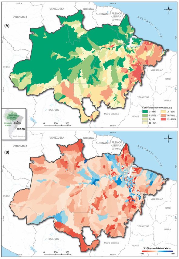
Water 2019, 11, 566 3 of 18
Water 2019, 11, x FOR PEER REVIEW 3 of 18
contamination
contamination[35,36].
[35,36].This
Thisregion
region possesses
possesses 40% of the living
living species
species on
on the
theplanet
planet[35,37],
[35,37],and
andowns
owns
the world’s largest freshwater reserves [38].
the world’s largest freshwater reserves [38].
Figure1.1.Amazon
Figure Amazonbiome
biomestudy
study area,
area, Landsat
Landsat scenes (n = 194) and
= 194) and the
the map
map sheets
sheets(n
(n==294)
294)used
usedfor
for
producing
producingannual
annualmosaics
mosaicsofofLandsat
Landsattotomap
map annually
annually surface
surface water from 1985 to 2017.
2.2.
2.2.Landsat
LandsatDataset
Dataset
We
Wehavehaveanalyzed
analyzedLandsat
LandsatData
Data Archive
Archive (LDA)
(LDA) [39] available in
[39] available in the
the Earth
Earth Engine,
Engine,covering
coveringthethe
period
periodofof1985
1985to to2017,
2017,totomap
map andand analyze
analyze thethe dynamics
dynamics of of surface water. A
surface water. A total
totalofof194
194Landsat
Landsat
scenes cover the study area (Figure 1). This tropical region is subject to persistent and
scenes cover the study area (Figure 1). This tropical region is subject to persistent and extensive cloud extensive cloud
cover [26]. Due to this cloudy condition, which blocks Landsat ground observation,
cover [26]. Due to this cloudy condition, which blocks Landsat ground observation, we have we have produced
an annual mosaic
produced an annual to remove
mosaic to clouds
remove using a median
clouds using astatistical filter available
median statistical in the Earth
filter available in theEngine.
Earth
The mosaic area covers the tile boundary of the International Map of the
Engine. The mosaic area covers the tile boundary of the International Map of the World to theWorld to the Millionth on
the scale of 1:250,000, comprising 1 ◦ 300 of longitude by 1◦ of latitude (Figure 1). Each mosaic requires
Millionth on the scale of 1:250,000, comprising 1°30′ of longitude by 1° of latitude (Figure 1). Each
two to four
mosaic Landsat
requires twoscenes
to fourand a totalscenes
Landsat of 294andmap mosaics
a total aremap
of 294 necessary
mosaics toare
cover the Amazon
necessary Biome
to cover the
boundary.
Amazon Biome We produced
boundary. the
We map sheet annual
produced the map mosaics with L1T
sheet annual Surface
mosaics withReflectance
L1T Surfacefor Landsat 5
Reflectance
(USGS, Sioux5 Falls,
for Landsat (USGS, SD, U.S.)
Sioux (1885–2002),
Falls, Landsat 7 (USGS,
SD, U.S.) (1885–2002), LandsatSioux Falls,Sioux
7 (USGS, SD, U.S.)
Falls,(2000–2015) and
SD U.S.) (2000–
Landsat
2015) and 8 (USGS,
Landsat Sioux Falls, SD,
8 (USGS, SiouxU.S.) (2013–2017),
Falls, pre-processed
SD, U.S.) (2013–2017), by USSG. Thebyannual
pre-processed USSG.timeframe
The annual for
image acquisition
timeframe for imageconcentrated
acquisitionmostly between
concentrated June 1st
mostly and October
between June 1st31st—the
and Octobermonths most months
31st—the likely to
most ground
allow likely tomeasurements
allow ground measurements
from the Landsat from the Landsat
sensors [26]. sensors [26].
2.3.
2.3.Image
ImageProcessing
Processing
WeWeselected
selected and processed
processedthe
theLandsat
Landsatimages
images directly
directly in the
in the Earth
Earth Engine
Engine Platform
Platform [28].
[28]. The
The image
image processing
processing steps
steps for mapping
for mapping surface
surface waterwater are summarized
are summarized in Figure
in Figure 2 and presented
2 and presented in detailin
detail
below.below.
Step 1: Build the annual Landsat mosaic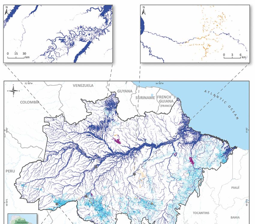
Water 2019, 11, 566                                                                                4 of 18

Step 1: Build the annual Landsat mosaic
      We searched and filtered the ortho-rectified L1T (Level 1 Terrain) Landsat collections based on
sensor type, year of acquisition, the time period of the year (i.e., June 1st through October 31st) and
cloud cover up to 30%. This procedure results in a list of Landsat scenes for each map sheet for each
year from 1985 to 2015. Next, we applied the pixel quality band of the Landsat sensors to map and
mask out clouds. A median statistical reducer was then used to estimate the best pixel observation
for the year. We also removed the edges of the Landsat scenes, prior to the application of the median
filter, using a 500 m buffer to avoid the inclusion of spurious data. Cloudy pixels not detected by the
pixel quality cloud mask were removed using the Cloud fraction (≥10%; see Step 2: Spectral Mixture
Analysis (SMA)). This process resulted in an annual mosaic of Landsat images with surface spectral
information for the period selected (i.e., June 1st through October 31st) (Figure 2).
Step 2: Spectral Mixture Analysis (SMA)
     SMA is a well-established image-processing tool for estimating the sub-pixel composition of
Landsat pixels [40], and applications have been proposed for mapping surface water bodies and
wetlands [40,41]. Here, we used annual median surface reflectance mosaics, with Landsat bands
1–5 and 7 obtained in Step 1, to estimate the Landsat pixel composition. The SMA model was used
to calculate the proportion of purer spectral signature (named endmembers) of Green Vegetation
(GV), Soil, Non-Photosynthetic Vegetation (NPV) and Cloud in each pixel, based on a generic set of
endmembers previously defined [42]. The SMA procedure was implemented in the Earth Engine using
the available unmixing algorithm, resulting in fractional or composition images of each endmember.
We calculated the shade fraction by subtracting the sum of all endmember fractions from 1 (i.e., 100%).
Therefore, the sum of all endmember fractions equals 1. Details of the SMA model and endmembers
used in this study can be found elsewhere [17,42].
Step 3: Surface Water Sub-Pixel Classification (SWSC)
     The fraction images obtained in Step 3 through the SMA model were used as inputs for Surface
Water Sub-Pixel Classifier (SWSC) to generate surface water maps. Surface water pixels have a high
fractional Shade value (i.e., >65%). The Soil fraction can increase in water with high content of
sediments (i.e., Soil), and sandbanks or bare ground along the border of rivers, lakes and wetlands.
GV composition is also expected to increase in floodplains, in wetlands and along the margins of rivers
and lakes. The SWSC uses simple binary decision rules to classify pixels (not blocked by clouds) as
surface water and no surface water, as follows (Figure 2):

     Surface Water: Shade ≥ 65% and (Soil + Vegetation) ≤ 20%.
     Land: otherwise

       Pixels with more than 10% of Cloud fraction were masked out to remove remaining cloudy
pixels not detected by the forest masking procedure described above. These simple binary rules were
applied to all fractional images of each annual mosaic with a threshold value for Shade varying slightly
(i.e., 1%–5%), across space and time due to changes in illumination in the Landsat scenes (Figure 2).
Step 4: Post-Classification
     We applied three post-classification procedures to the annual surface water maps obtained with
the SWSC. First, we used spatial filtering to remove spurious classification results. This spatial filter
uses a region-labeling algorithm available in the Earth Engine to identify each contiguous surface
water bodies or objects. Surface water objects with less than three pixels were removed from each
annual map of surface water because they were too small to be classified as water bodies. We then
applied a temporal moving window filter with a kernel size of three, to reclassify Cloud if the
previous and the subsequent years belong to the same class (i.e., Land or Surface Water). Finally,
we also produced a Water Occurrence map as proposed by [23] to characterize and quantify the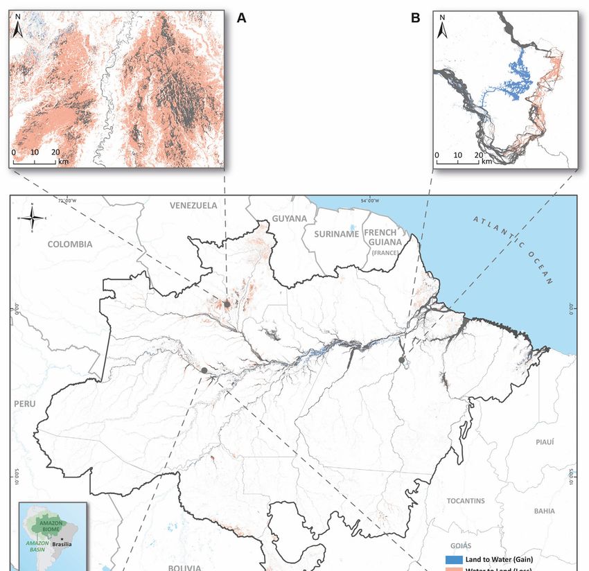
Water 2019, 11, 566                                                                                         5 of 18

Water 2019, 11, x FOR PEER REVIEW                                                                          5 of 18
 frequency of Surface Water mapping between 1985 and 2017. Next, we reclassified the pixels that were
surface. This
 classified   procedure
            less than 10%allowed   removal
                           of the time (i.e., of
                                              ~3misclassification
                                                 years) as surfaceofwater
                                                                     surface water
                                                                          over     associated
                                                                               the 33 years aswith
                                                                                              Landburned
                                                                                                   surface.
areas
 This and  high shade/shadow
      procedure                 in urban
                  allowed removal          areas.
                                    of misclassification of surface water associated with burned areas and
 high shade/shadow in urban areas.

       Figure 2. Image processing applied to annual Landsat datasets acquired between June and October
     Figure  2. Image
       to derive      processing
                  surface         applied
                          water maps,     to annual
                                        (A)  annual median
                                                    Landsat mosaic
                                                            datasets(B)
                                                                      acquired  between
                                                                         SMA color       June and(Red—Soil,
                                                                                       composite   October
     toGreen—Green
        derive surfaceVegetation,
                        water maps,   (A) annual(C)
                                  Blue—Shade),    median
                                                    surfacemosaic  (B) SMA color
                                                            water classification, andcomposite (Red—Soil,
                                                                                      (D) temporally  filtered
     Green—Green
       surface water.Vegetation, Blue—Shade), (C) surface water classification, and (D) temporally filtered
     surface water.
 2.4. Surface Water Object Classification
2.5. Surface Water
       Isolating   Objectwater
                 surface Classification
                               objects was necessary to classify them into natural and artificial surface
  water  bodies.surface
      Isolating  For that, we applied
                        water          the region
                               objects was        labeling
                                            necessary      algorithm
                                                      to classify    available
                                                                  them         in theand
                                                                       into natural   Google  Earthsurface
                                                                                         artificial Engine,
water bodies. For that, we applied the region labeling algorithm available in the Google Earth Engine,
first to isolate the surface water objects and assign them a unique identifier or label. Next, we
calculated the area of each water object and extracted their morphological attributes including area,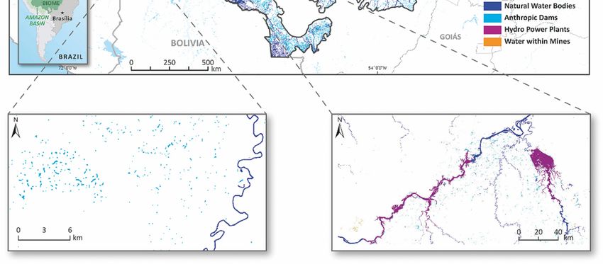
Water 2019, 11, 566                                                                                   6 of 18

first to isolate the surface water objects and assign them a unique identifier or label. Next, we calculated
the area of each water object and extracted their morphological attributes including area, perimeter,
area-perimeter ratio and convexity/concavity degree. The area and morphological attributes of the
water bodies were used as data features to train and run a random forest classifier (with 100 trees) to
classify the following surface water classes:

     Natural: rivers, lakes, wetlands.
     Anthropic: hydroelectric dams, small dams, and gold mining.

2.5. Characterization of Surface Water Dynamics
     We evaluated surface water dynamics at the Amazon Biome (Figure 1) and watershed scales.
To do that, we measured annual variability of surface water extent mapped with the SWSC, and the
changes from Land to Water (i.e., gain) and Water to Land (loss). The watershed analysis allowed
us to account for regional variations in gains and losses of surface water during the timeframe of
this study (1985–2017). We also quantified the extent of annual surface water in each watershed.
We used level 4 watershed boundary [43] made available the federal hydrographical institution of
Brazil (i.e., ANA—Agência Nacional de Águas). Furthermore, we calculated for each watershed the
mean surface water area from 1985 to 2017, and estimated the percent change from the mean for each
watershed to assess which watersheds had gains and losses in surface water in 2017.

2.6. Deforestation Impact on Surface Water
       We combined spatially explicit deforestation data from Prodes, the Brazilian Amazon Forest
Monitoring Program, with surface water derived from SWSC and the types of water body objects
(i.e., Natural and Anthropic). This spatial analysis covered a shorter period (i.e., 2000–2017) because
Prodes annual digital maps are available only after 2000. Next, we analyzed the amount and size of
artificial yearly mapped water bodies (hydroelectric dams, small dams, and gold mining) inside the
annually deforested areas. This deforestation analysis was also conducted at the watershed scale to
assess correlation with surface water extent. For that, we analyzed the effect of deforestation and forest
cover in surface water area using a linear mixed model applied to classes of watersheds that gained
and lost surface water (see Section 2 of Supplementary Materials).

2.7. Accuracy Assessment
      We estimated the accuracy statistics for Land and Water classes for each year from 2000 to 2015
using 1000 stratified random sample points. We used Landsat color composites and asked three
independent image analysts to classify the sample points based on visual interpretation of three classes:
Water, Land or Cloud. Next, we generated a final reference dataset combining the results from the three
analysts results using a majority rule, i.e., assign the final class when more than two analysts agreed
(see [44] for more details) and removing sample points classified as Cloud. The average number of
total points evaluated per year was 838 (s = 75) after removal of unobserved pixels, with 93 (s = 6) for
Water, and 745 (s = 78) for Land. Accuracy statistics were calculated using area-adjusted corrections,
proposed as a best-practice procedure by the literature [45].

3. Results and Discussion

3.1. Surface Water Classification
     The SWSC algorithm applied to SMA fractions derived a long-term (i.e., 33 years) dataset of annual
surface water for the Amazon Biome. This annual mapping focused on the dry season (circa June 1st,
through October 31st), which increases the likelihood of acquiring Landsat images in the Amazon
region with less cloud [26], allowing annual map a large extent of the study area. Due to a lower
precipitation regime during this period of the year [43], the surface water detected is expected to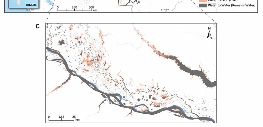
Water 2019, 11, 566                                                                                                   7 of 18

capture the lowest water level of rivers, lakes and flood plains (although torrential rainfall can generate
Water 2019, 11, x FOR PEER REVIEW                                                                                     7 of 18
localized flooding during the dry season). We also processed the GSW dataset and generated monthly
statistics of the surface
optimal period      to monitorwater   extent,water
                                   surface     which  revealed
                                                    with  opticalthat  GSW mapped
                                                                    Landsat              less surface
                                                                               data is between    Junewater    during the
                                                                                                         and October,     as
rainy  season    relative
applied in this study.     to  the  dry  season  (Figure  S3).  This  suggests    that the  optimal   period   to  monitor
surface
      Thewater
           Landsatwithmedian-reduced
                         optical Landsat mosaic
                                             data is between
                                                     for 2017 June    and October,
                                                                generated              as applied
                                                                              normalized            in this study.
                                                                                             SMA fraction    images over
      The  Landsat     median-reduced        mosaic  for 2017   generated     normalized     SMA   fraction
the 33-year timespan of this study. Figure 3 shows a subset of this dataset as an example of the image       images    over
the 33-year    timespan    of  this study.   Figure 3 shows   a  subset  of  this dataset  as
processing techniques applied to the Landsat dataset. Surface water bodies show up as dark bluean example    of  the image
processing
colors in SMA techniques
                    fractionapplied      to the Landsat
                               color composites           dataset.
                                                    of Soil           SurfaceVegetation
                                                            (Red), Green        water bodies     showand
                                                                                             (Green)    up Shade
                                                                                                             as dark(Blue)
                                                                                                                       blue
colors  in  SMA     fraction   color   composites   of Soil (Red),    Green    Vegetation    (Green)
providing high contrast with land cover categories (i.e., forest, agriculture and urban lands) (Figure and  Shade    (Blue)
providing    high contrast
3A). The application          withbinary
                           of the    land cover  categories
                                           hierarchical      (i.e.,
                                                         rules      forest,
                                                                of the  SWSCagriculture
                                                                                 algorithmandtourban  lands) (Figure
                                                                                                the Landsat             3A).
                                                                                                               time-series
The  application
fractions   produced  of the  binary
                          annual    mapshierarchical
                                            of Surfacerules of the
                                                        Water    andSWSC       algorithm
                                                                       Land (Figure     3B).toCombining
                                                                                               the Landsatthese
                                                                                                              time-series
                                                                                                                    annual
fractions   produced      annual    maps    of Surface  Water   and   Land    (Figure   3B).
surface water maps allowed us to generate frequency or water occurrence maps of surface water Combining     these   annual
surface
betweenwater
           1985 andmaps2017allowed
                              (Figureus   to The
                                        3C).  generate  frequency
                                                  average             or waterofoccurrence
                                                           user’s accuracy                      maps of surface
                                                                                   the SWSC algorithm       throughwater
                                                                                                                       2000
between
to 2015 was 95% (s = 1), with 84% (s = 2) average user accuracy for the Water class, and 96% (s = 1)2000
           1985   and  2017   (Figure   3C).  The average  user’s    accuracy   of the SWSC     algorithm   through      for
to
the2015
    Land.was 95% (s = 1), with 84% (s = 2) average user accuracy for the Water class, and 96% (s = 1) for
the Land.

      Figure 3. Example of Spectral Mixture Analysis (SMA) results for a portion of the Amazonas River
      Figure 3. Example of Spectral Mixture Analysis (SMA) results for a portion of the Amazonas River
      and Tapajós tributary. In (A), a color composite obtained by combining fraction images of Soil (Red),
      and Tapajós tributary. In (A), a color composite obtained by combining fraction images of Soil (Red),
      Green Vegetation (Green) and Shade (Blue). In (B), the water classification based on the surface water
      Green Vegetation (Green) and Shade (Blue). In (B), the water classification based on the surface water
      sub-pixel classifier (SWSC) and in (C) the water frequency map over 33 years. Light blue areas adjacent
      sub-pixel  classifier
      to dark blue  ones are(SWSC)
                              likely toand  in (C) land
                                        represent   the water  frequency map
                                                        areas susceptible        over 33and
                                                                           to flooding,   years. Light
                                                                                            bright  blueblue areas
                                                                                                         areas can
      adjacent
      also designate areas that had the fewer cloud-free satellite observation such as in the left side ofblue
                to dark  blue ones  are  likely to represent land  areas susceptible to flooding, and  bright  the
      areas
      Figurecan
              3C.also designate areas that had the fewer cloud-free satellite observation such as in the left
      side of the Figure 3C.
     We estimated the annual surface water area from the SWSC maps (Figure 4). The maximum
     Wewater
surface   estimated   the annual
                 mapped           surface
                          was in 1991     water area
                                       covering       from
                                                 an area  of the SWSC
                                                             almost     mapskm
                                                                    140,000   (Figure 4). The
                                                                                2 and the     maximum
                                                                                          minimum  one
surface water   mapped   was  in
                               2 1991 covering an area of almost  140,000 km2 and the minimum one was
was in 2016 (i.e., 108,674 km ), which is considered an extremely dry year in the Amazon region [44].
in 2016 (i.e., 108,674 km2), which is considered an extremely dry year in the Amazon region [44]. The
range in surface water between 1991 and 2016 was 30,838 km2. However, surface water mapped in
2016 is also 16,180 km2 below the average surface water mapped from 1985 to 2017 (i.e., 33 years)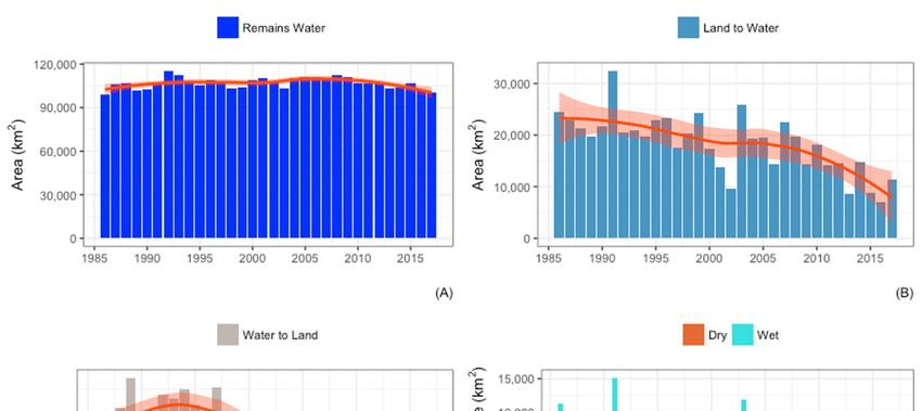
Water 2019, 11, 566 8 of 18
The
Waterrange inxsurface
2019, 11, FOR PEER water
REVIEW between 1991 and 2016 was 30,838 km2 . However, surface water mapped 8 of 18
2
in 2016 is also 16,180 km below the average surface water mapped from 1985 to 2017 (i.e., 33 years)
(Figure 2
(Figure 4A).
4A). TheThe second
second lowest
lowest surface
surfacewater
watermapped
mappedwas wasinin1985
1985(112,599
(112,599km
km2/year).
/year). Surface water
extent also varied throughout the decades.
the decades.
We also
also estimated
estimated the the minimum,
minimum, maximum, mean and the standard deviation (s) of surface
water for circa decade periods (Figure 4B, Table Table 1).
1). The average surface water between 1985 and 1989
was 123,274 km22/year /year(s(s= =5997).
5997).TheThe largest surface water
largest surface water extent
extent mapped
mapped waswas in the
in the 1990s
1990s withwith
an
an average of 130,379 2
average of 130,379 kmkm2 /year/year (s = 5302),
(s = 5302), followed
followed by aby a decrease
decrease in surface
in surface waterwater
in theinearly
the early
2000s2000s
and
and an increase in 2005. 2 /year
an increase in 2005. The The average
average surface
surface water
water mappedmapped during
during the the 2000s
2000s waswas 127,265
127,265 kmkm
2/year (s =
(s = 4593), which is slightly lower than the average for the 1990s (Figure 4B).
4593), which is slightly lower than the average for the 1990s (Figure 4B). However, after 2010, a However, after 2010,
aconstant
constantannual
annual decrease
decrease in insurface
surfacewater
waterwas
wasdetected (Figure
detected 4A).4A).
(Figure Between 2010 and
Between 20102017,
and the SWCS
2017, the
detected the lowest average of surface water in the Amazon Biome relative to
SWCS detected the lowest average of surface water in the Amazon Biome relative to the past threethe past three decades,
falling to falling
116,811tokm 2 /year (s 2= 5702) (Figure 4B Table 1).
decades, 116,811 km /year (s = 5702) (Figure 4B Table 1).
Figure
Figure 4. Annual surface
4. Annual surface water
water extent
extent mapped
mapped with
with SWSC
SWSC with
with Loess
Loess trend
trend smooth
smooth pattern
pattern (red
(red line)
line)
and 95% confidence interval (A). Box plot statistics are presented in (B) for circa decade periods.
and 95% confidence interval (A). Box plot statistics are presented in (B) for circa decade periods.
Table 1. Surface water mapping summary statistics estimated for decade periods.
Table 1. Surface water mapping summary statistics estimated for decade periods.
Minimum Maximum Mean
Period (# Years) Minimum Maximum Mean Standard Deviation (s)
Period (# Years) 2
(km 2) (km22 /year) Standard Deviation (s)
(km ) (km /year)
1985–1989
1985–1989 112,599
112,599 129,072
129,072 123,274
123,274 5997
5,997
1990–1999 123,325 139,512 130,379 5302
1990–1999
2000–2009
123,325
117,396
139,512
132,498
130,379
127,265
5,302
4593
2000–2009
2010–2017 117,396
108,674 132,498
124,923 127,265
116,811 4,593
5702
2010–2017 108,674 124,923 116,811 5,702
3.2. Surface Water Dynamics
3.2. Surface Water Dynamics
Investigating annual surface water change can help to explain the overall trend in the decreasing
yearlyInvestigating
surface waterannual
extentsurface water
detected change
during canseason
the dry help toofexplain the overall
the Amazon trend
region. Theinmost
the decreasing
significant
yearly surface
reduction water
in surface extent
water detected
happened during
in the 2010sthe
withdry season
almost of km
13,000 the2 of
Amazon region.
difference The water
in surface most
significant reduction in surface water happened in the 2010s with almost 13,000 km 2 of difference in
between 2010 and 2017 (i.e., ~10%; Figure 4). A 10% reduction in average surface water extent between
surface
the 1990swater
and between
the 2010s2010
was and
also 2017 (i.e., ~10%;
observed (TableFigure
1), but 4). A 10% reduction
a constant decrease in in average surface
the surface waterwater
was
extent between the 1990s and the 2010s was
the overall spatiotemporal pattern after 2010. also observed (Table 1), but a constant decrease in the
surface water was the overall spatiotemporal pattern after 2010.
We characterized the surface water dynamics by decoupling annual changes between Water to
We characterized the surface water dynamics by decoupling annual changes between Water to
Land and Land to Water from areas that remained as water (Figure 5). The results of the decoupling
Land and Land to Water from areas that remained as water (Figure 5). The results of the decoupling
analysis of surface water change showed that areas mapped in the Remains Water class did not
analysis of surface water change showed that areas mapped in the Remains Water class did not show
the overall trend of decreasing surface water over the period investigated (i.e., 1985 through 2017).
The average surface area in this class of water was around 100,000 km2/year (i.e., 2.4% of the Amazon
Biome). However, areas that changed from Land to Water, and from Water to Land showed a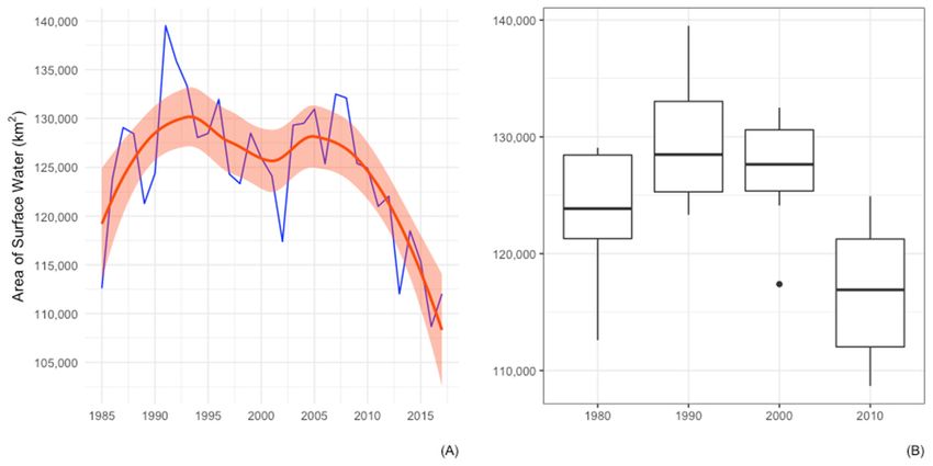
Water 2019, 11, 566 9 of 18
show the overall trend of decreasing surface water over the period investigated (i.e., 1985 through
2017). The11,average
Water 2019, x FOR PEERsurface area in this class of water was around 100,000 km2 /year (i.e., 2.4%
REVIEW of
9 of 18
the Amazon Biome). However, areas that changed from Land to Water, and from Water to Land
decreasing
showed trend in surface
a decreasing trend inwater extent
surface (Figure
water extent5B,C) as detected
(Figure 5B,C) as in the total
detected insurface water
the total mapped
surface water
annuallyannually
mapped (Figure 3A). The3A).
(Figure rateThe
of change over 33 over
rate of change years33obtained with a linear
years obtained with aregression model
linear regression
showed
model a decrease
showed in surface
a decrease in water extent
surface waterof 350 km2of
extent /year
350over
km2the
/year33-year
overtimespan in the
the 33-year areas that
timespan in
the areas that underwent an interchange between landmass and water. We observed thatand
underwent an interchange between landmass and water. We observed that between 1985 2000
between
these
1985 annual
and changes
2000 these werechanges
annual not pronounced, but after thatbut
were not pronounced, point
afterinthat
time, we in
point detected
time, we a constant
detected
decrease in the extent of Land to Water and Water to Land changes (Figure 5B,C).
a constant decrease in the extent of Land to Water and Water to Land changes (Figure 5B,C). However, However, the
fastest shrinkage of the areas subjected to this type of dynamics happened between
the fastest shrinkage of the areas subjected to this type of dynamics happened between 2010 and 2017, 2010 and 2017,
withan
with anaverage
averagedecrease
decreaseofofnearly
nearly1400
1400km
km22/year.
/year.
Figure5.5.Annual
Figure Annual decoupling
decoupling of
of annual
annual surface area mapped
surface area mapped inin the
the class
class Remains
RemainsWater
Water(A)
(A)from
from
changes from Land to Water (B), Water to Land (C), and annual net difference (D) between the classes
changes from Land to Water (B), Water to Land (C), and annual net difference (D) between the classes
inin(B,C).
(B,C).
The 2
Theaverage
averagechange
changefrom fromLand
Landto toWater
Waterwas was19,622
19,622kmkm2/year over the
/year over the 33-year
33-yeartimespan
timespanof ofthis
this
analysis
analysis(Figure
(Figure5B). We
5B). We expected
expected to to
detect thethe
detect peak of this
peak typetype
of this of change in the
of change in years of flooding
the years areas
of flooding
by hydroelectric dams inundation, but our time-series analysis did not reveal
areas by hydroelectric dams inundation, but our time-series analysis did not reveal that signal that signal because this
analysis was conducted on the biome scale. More spatially detailed analysis (i.e., at
because this analysis was conducted on the biome scale. More spatially detailed analysis (i.e., at the the micro-watershed
level) was also conducted
micro-watershed level) wasandalso
is presented
conducted in the
andfollowing section.
is presented in theFlooding
following of natural
section.landmasses
Flooding of in
floodplains and along the borders of rivers and lakes makes are areas more
natural landmasses in floodplains and along the borders of rivers and lakes makes are areas more subject to Land to Water
changes. Moreover,
subject to Land to extreme-flooding events were
Water changes. Moreover, also not detected
extreme-flooding at thewere
events Amazon also Biome scale. In
not detected at2012,
the
for example,
Amazon an extreme
Biome scale. Inflooding event
2012, for hit the port
example, of the city
an extreme of Manaus,
flooding eventincreasing
hit the port the of
water
the level by
city of
almost 30 m for more than two months [46,47], and an intense rainfall occurred
Manaus, increasing the water level by almost 30 m for more than two months [46,47], and an intense in 2009 [48]. None of
these extreme-flooding
rainfall occurred in 2009 events
[48]. are
Noneevident (Figure
of these 4B) at the Biome
extreme-flooding scale.
events areWe have also
evident observed
(Figure 4B) at that
the
the average
Biome scale.annual area
We have that
also had interchange
observed between
that the average waterarea
annual andthat
land before
had 2010 (i.e.,
interchange km2 )
~40,000water
between
reduced
and land bybefore
half in2010
2017(i.e.,
(Figure 5B,C).
~40,000 km We did not observe
2) reduced by half opposite trends between
in 2017 (Figure 5B,C). WeLand did tonotWater and
observe
opposite
Water trends
to Land between
because Land
these to Wateroccur
processes and Water to Land
in different because
regions thesethe
across processes
Amazonoccur Biome.in different
regions across the Amazon Biome.
The annual net difference of areas that interchanged between land and water may be more
indicative of climatic extremes at the Biome scale (Figure 5D). This net difference can be an indicator
of whether surface water expanded or reduced more in a given year, revealing an overall wet or dry
Water 2019, 11, 566                                                                               10 of 18

     The annual net difference of areas that interchanged between land and water may be more
indicative of climatic extremes at the Biome scale (Figure 5D). This net difference can be an indicator
of whether surface water expanded or reduced more in a given year, revealing an overall wet or
dry condition in the Amazon region. The SWSC algorithm detected more surface water expansion
in the 1980s, 1990s, and 2000s, and less in 2010s (Figure 5D). In 1995 and 2005, years reported as
having a deficit in rainfall [14], we observed a small net increase in areas changing from Land to Water.
However, in 1997–1998, 2010 and 2016, years of extreme drought, we detected a net increase in areas
changing from Water to Land.
     We also analyzed the net difference of areas that interchanged between land and water between
1991 and 2017. These were the years that exhibited the highest and lowest surface water extent,
respectively (Figure 4). The majority of the water to land change occurred in wetlands and flood plains
along rivers and lakes (Figure 6). The interchange between water and land occurred, for example,
with the construction of the Belo Monte hydroelectric dam (Figure 6), where gains in water occurred in
the land area that was inundated, and losses in water happened in areas where the Belo Monte dam
change their natural course (Figure 6). We conducted this same type of analysis using the GSW dataset
and did not observe the changes presented in Figure 6 (see Figure S5).

3.3. Characterization of Surface Water Types
      Surface water bodies were isolated and classified as Natural or Anthropic. The Anthropic surface
water bodies were then sub-classified into Hydroelectric Dams, Agricultural Dams and Water in
Mining (i.e., mostly gold mining operations). The Natural water bodies included large and small
rivers, lakes and floodplains, but no attempt was made to separate these classes due to computational
challenges in processing vector data in the Earth Engine.
      Natural water bodies had an average surface area of 118,084 km2 /year (s = 7804) between 2000
and 2017, which is the period in which we analyzed the impact of deforestation on surface water. The
statistical range for this class of surface water was 25,367 km2 with the extremes in 2007 (125,845 km2 )
and 2016 (100,478 km2 ) (Figures 7 and 8A). The year 2016 is considered a “record-breaking warming”
due to the extreme drought associated with El-Niño [49], and we found again a signal that shows
a potential drought effect on the extent of surface water at Biome scale. We also found that the five
lowest extents of Natural surface water happened between 2013 and 2017, the warmest decade in
post-industrial history [14,50].
      The area of Anthropic water bodies increased between 2000 and 2017 (Figures 7 and 8). We have
identified three types for this class of water bodies: Hydroelectric Dams, Agriculture Dams and Water
in Mining. The maximum extent of surface water for the Anthropic water bodies was detected in
2017, when it was 8831 km2 (Figure 8), which represents a 28% increase relative to the average for
this period (6899 km2 /year). The sub-classification of Anthropic water bodies showed that the area
of Hydroelectric Dams was around 6000 km2 between 2000 and 2010, but quickly increased after
2010, reaching 7467 km2 in 2017 (i.e., ~85% of the surface area of Anthropic water bodies). However,
Agriculture Dams have increased steadily between 2000 and 2017, from 457 to 1223 km2 , respectively
(Figure 8C). The surface water extent of Agriculture Dams represents almost 14% of the total Anthropic
water bodies in 2017, and this class spatially correlates with deforestation, with more than 50,000 small
dams detected. The concentration of small agriculture dams also followed the spatial pattern of the
main roads along the Transamazon and Santarém-Cuiaba highways (Figure 7).
Water 2019, 11, 566 11 of 18
Water 2019, 11, x FOR PEER REVIEW 11 of 18
Figure 6.
Figure Interchange between
6. Interchange between water
water and
and land
land detected
detected between
between 1991
1991 and
and 2017,
2017, which
which are
are the
the highest
highest
and lowest surface water extent, respectively. Orange areas represent areas that changed from water
and lowest surface water extent, respectively. Orange areas represent areas that changed from water in
1991 to land in 2017, and blue ones are changes from land to water between these years. In panel (A)
in 1991 to land in 2017, and blue ones are changes from land to water between these years. In panel
wetlands changed from Water to Land; in (B) Land to Water associated with the construction of Belo
(A) wetlands changed from Water to Land; in (B) Land to Water associated with the construction of
Monte hydroelectric dam and Water to Land along the rivers that had the water flow diverted by the
Belo Monte hydroelectric dam and Water to Land along the rivers that had the water flow diverted
dam construction; and in (C) mostly Water to Land in flood plains along lakes and rivers.
by the dam construction; and in (C) mostly Water to Land in flood plains along lakes and rivers.
The map of Anthropic water bodies revealed a spatial pattern that links fragmentation of small
The map of Anthropic water bodies revealed a spatial pattern that links fragmentation of small
rivers with the Amazon Arc of Deforestation (Figure 7). Hydroelectric Dams are a well-known driver
rivers with the Amazon Arc of Deforestation (Figure 7). Hydroelectric Dams are a well-known driver
of fragmentation of large rivers dramatically affecting freshwater connectivity [9,51]. Fragmentation of
of fragmentation of large rivers dramatically affecting freshwater connectivity [9,51]. Fragmentation
small streams has not been documented yet at a large scale such as in the Amazon Biome. A study at the
of small streams has not been documented yet at a large scale such as in the Amazon Biome. A study
local level of the Paragominas municipality, in the Eastern Amazon, revealed high rates of deforestation
at the local level of the Paragominas municipality, in the Eastern Amazon, revealed high rates of
in riparian permanent preservation areas, which are meant to protect small rivers and maintain forest
deforestation in riparian permanent preservation areas, which are meant to protect small rivers and
maintain forest and water connectivity [52]. Our results showed that deforestation in riparianWater 2019, 11, 566 12 of 18
Water 2019, 11, x FOR PEER REVIEW 12 of 18
and water connectivity [52]. Our results showed that deforestation in riparian permanent preservation
permanent preservation
areas is happening areas
in a much is happening
larger in aAmazon
area across the much larger area across the
Arc of Deforestation dueAmazon Arc of
to large number
Deforestation due to large number
of dams along small streams (Figure 7).of dams along small streams (Figure 7).
Finally, we detected
Finally, we detected only
only 140
140 km
km22 of
of surface
surface water
water in
in the
the Water
Water in
in Mining
Mining class,
class, which
which represents
represents
1.5% of
1.5% of the
the total
total Anthropic
Anthropic water
water bodies
bodies mapped
mapped until
until 2017
2017 (Figure
(Figure 8C).
8C). This
This class
class is
is mostly
mostly
concentrated
concentrated mostly in the Tapajós watershed in Southwestern Pará, but there are scattered spots of
mostly in the Tapajós watershed in Southwestern Pará, but there are scattered spots of
Water in Mining
Water in Mining in
in Roraima,
Roraima, Rondonia
Rondonia andand Mato
Mato Grosso
Grossostates
statesas
aswell
well(Figures
(Figures77and
and8C).
8C).
Figure 7. Surface water types mapped for the entire Amazon Biome in 2007. The panels depict
Figure 7. Surface water types mapped for the entire Amazon Biome in 2007. The panels depict
examples of hydroelectric dams (bottom-right), small stream fragmentation in the Arc of Deforestation
examples of hydroelectric dams (bottom-right), small stream fragmentation in the Arc of
(bottom-left), Natural surface water (top-left) and mining along rivers (top-right).
Deforestation (bottom-left), Natural surface water (top-left) and mining along rivers (top-right).Water
Water 2019,
2019, 11, 11,
566x FOR PEER REVIEW 1318
13 of of 18
Figure 8. Absolute (A) and relative (B) surface water types showing a decrease in Natural water bodies,
andFigure 8. Absolute
an increase (A) and
in Anthropic relative
ones. (B) surface
Hydroelectric water
Dams typesanshowing
showed a decrease
increase in in Natural
surface water water
after 2010,
bodies, and an increase in Anthropic ones. Hydroelectric
and Agriculture Dams steady growth since 2000 (C). Dams showed an increase in surface water
after 2010, and Agriculture Dams steady growth since 2000 (C).
3.4. Potential Drivers of Surface Water Change
3.4. Potential Drivers of Surface Water Change
The surface water dynamics at the watershed scale showed a trend of decreasing surface water for
The surfacewith
most watersheds, water dynamics
some showingatan theincrease
watershed trend scale showed
(Figure a trend
9). Figure 9Aofshows
decreasing surface water
the proportion of
for most watersheds,
deforestation with some
within watersheds, showing
with green areasanrepresenting
increase trend (Figurewith
watersheds 9). high
Figure 9Acover
forest shows andthe
lowproportion of deforestation
level of deforestation, and within watersheds,
yellow-red colors high withdeforestation
green areas representing
and low forestwatersheds
cover (Figure with9A).
high
Theforest cover
percent and low
of losses andlevel
gainsoffrom
deforestation,
the averageand yellow-red
surface colors 1985
water during high anddeforestation and for
2017 is shown low2017
forest
cover9B).
(Figure (Figure
These9A).
mapsTherevealed
percentthat of losses
most of andthegains from the
watersheds hadaverage surfacewater
their surface waterreduced
during in 1985
both and
2017
high is shown forand
deforestation 2017high
(Figure 9B).
forest These
cover maps revealed
conditions (Figure that
9),most of thethat
implying watersheds hadcorrelation
there is no their surface
water reduced
between both (i.e.,inthere
bothishigh deforestation
reduced surface water and high forest of
regardless cover conditions
the forest cover(Figure 9), implying that
and deforestation).
there
Theisstatistical
no correlation betweenthat
test reviewed boththe (i.e., there
effect ofisdeforestation
reduced surface water regardless
on surface water change of the
was forest cover
slightly
but was stronger and more statistically significant (χ21 = 53.1; p = 0.0023) for the watersheds
and deforestation).
positive,
The statistical
that gained water than testfor
reviewed that the
watersheds thateffect
lost of deforestation
water (Table S1). on surface
The effect water
of change was slightly
forest cover was
positive,
stronger andbut wasstatistically
more stronger and significant (χ21 = 142.7;
more statistically significant
p < 0.00001) (߯ଵଶ than
= 53.1; p = 0.0023) for
deforestation, the watersheds
suggesting that
that gained
watersheds withwater
higher than forcover
forest watersheds
have lost that
more lostsurface
water water(Table(Table
S1). TheS2). effect of forest cover was
stronger and more
These results statistically
suggest significantthat
that watersheds (߯ଵଶhave
= 142.7;
highp forest
< 0.00001)
coverthan(i.e.,deforestation,
with minimalsuggesting
influence of that
watersheds
land use and land withcover
higher forest from
change coverdeforestation
have lost more insurface water (Table
infrastructure S2).
development) may have other
These results
factors driving suggest of
the reduction that watersheds
surface water. that
The GSW have dataset
high forest wascover (i.e., withtominimal
also analyzed influence
assess whether
of land
surface use and
water was land coverover
reducing change
time,from
but deforestation
this trend wasinnot infrastructure
detected. First, development)
GSW detected mayalso
have other
more
factors
surface driving
water the in
extent reduction
the dry of surface
season water.toThe
relative theGSW dataset was
wet season. also analyzed
A notched boxplottorevealed
assess whether
that
surface of
detection water was water
surface reducing over time,
in these seasons butwasthisstatistically
trend was not detected.
different First, S3).
(Figure GSWWe detected also more
also observed
surface
that GSW waterdid notextent
detectinland
the dry
and season relative to the
water interchange wet season.
as SWSC detected A notched
(Figure 6; boxplot revealed
see Figure that
S5 for
detection ofMost
comparison). surface waterchanges
of these in these are
seasons was statistically
associated with wetlands, different (Figure S3).
floodplains, andWe alsostreams,
small observed
that are
which GSW did water
mixed not detect land and
ecosystems water interchange
composed as SWSC and
of water vegetation detected
soils at (Figure 6; see Figure
the Landsat S5 for
pixel scale.
comparison).
This may explain Most
whyofGSW thesehas changes are associated
not detected the same with
trend wetlands,
of reducingfloodplains,
surface andwatersmall
afterstreams,
2010
as which
detected arebymixed
SWSC water ecosystems
because GSW does composed of water
not detect vegetation
information at and soils at thelevel.
the sub-pixel Landsat pixel scale.
Monitoring
This may
wetlands, explain why
floodplains andGSWsmallhas not detected
streams the same
are important trend of
because reducing
they are more surface water after
vulnerable 2010 as
to climate
detected
change [53].byFurther
SWSC investigation
because GSWis does not detect
necessary to assessinformation
whether at the sub-pixel
climate change can level. Monitoring
explain this
wetlands,
overall trendfloodplains
of decreasing and small water
surface streams are2010
after important
consideringbecause they are
external moresuch
drivers vulnerable to climate
as El Niño and
thechange
warming [53].
of Further investigation
the Atlantic North (Figureis necessary
4A). to assess whether climate change can explain this
overall trend of decreasing surface water after 2010 considering external drivers such as El Niño and
the warming of the Atlantic North (Figure 4A).Water 2019, 11, 566 14 of 18
Water 2019, 11, x FOR PEER REVIEW 14 of 18
Figure 9. Proportion
Figure 9. Proportionofofforest
forest(green) and
(green) deforested
and areas
deforested (orange)
areas at level
(orange) 4 watersheds
at level (A), and
4 watersheds (A),gains
and
and
gains and losses of surface water in 2017 per watershed relative to the mean difference from 1985(B).
losses of surface water in 2017 per watershed relative to the mean difference from 1985 to 2017 to
2017 (B).
4. Conclusions
We used Landsat images acquired during June and October for the years 1985 through 2017 to
4. Conclusions
map and estimate the annual extent of surface water across the Amazon Biome in Brazil with the novel
SWSC. We used
This Landsat
classifier hasimages acquired
as inputs duringabout
information Junewater
and October for the years
(as represented 1985 green
by shade), through 2017 to
vegetation
map and estimate the annual extent of surface water across the Amazon Biome
and soil endmembers found at the Landsat sup-pixel scale. The SWCS allowed detection and mapping in Brazil with the
novel
of SWSC.
large waterThis classifier
bodies has as
(i.e., river andinputs
lakes)information
also detectedabout
withwater
whole(aspixel
represented by such
classifiers shade),
as green
GSW.
vegetation and soil endmembers found at the Landsat sup-pixel scale. The SWCS
However, the SWSC identified more surface water in wetlands, floodplains along rivers and lakes, allowed detection
and in
and mapping
narrowof large water
streams, bodies
and also (i.e., river
allowed and lakes)
monitoring alsointerchange
annual detected with whole water
between pixel classifiers
and land.
such as GSW. However, the SWSC identified more surface water in wetlands,
These regions with high water dynamics are even more vulnerable to climate change (e.g., floodplains along rivers
[53,54]).
and lakes, and in narrow streams, and also allowed monitoring annual
The SWSC used a generic SMA model using an endmember library extracted from Landsatinterchange between water
datasets inThese
and land. a largeregions withdataset.
time-series high water dynamics
Therefore, this are evenhad
method morethevulnerable
potential totobe
climate
appliedchange (e.g.,
at a global
[53,54]).Water 2019, 11, 566 15 of 18
scale. However, water in wet forests cannot be detected, which limits the use of optical imagery to map
and monitor the full extent of surface water in the Amazon Biome. Landsat data also cannot monitor
this region over the entire year, being more suitable to be used in the dry season when clouds are less
abundant and frequent. The SWSC may be limited to monitor surface water in mountainous areas
since shadows can obscure and create ambiguity with surface water. Our future research will integrate
Sentinel 1 microwave data with optical data to improve monthly mapping and monitoring of surface
water. These types of application will become more relevant, given the ongoing extreme warming and
flooding events in this region.
The SWCS mapped an average of 130,000 km2 /year of surface water and detected a general
trend of reducing surface water after 2010, the warmest years in this region since the post-industrial
era in the Amazon [55]. This temporal trend of decreasing surface water was also visible in areas
undergoing more annual interchange between landmass and water. Natural surface water bodies also
had a decrease in extent over time. This process may be associated with a warming temperature trend
in the Amazon region [55], also revealed in more detailed analysis at the watershed scale. The fact
that watershed with high forest cover lost surface water over time may suggest that this process is
connected with climate change. However, other studies have found a general wetting trend in the
Amazon Basin [54,56], but our results suggest that during the dry season a drier trend has occurred in
this region since 2010.
Most of the surface water mapped in this study was associated with large rivers, lakes and
floodplains. Hydroelectric dams were found to have the largest area of surface water, with an increase
after 2010 due to new constructions. Small narrow streams were not visible in forested regions but
became distinct in the Arc of Deforestation where we detected more than 50,000 small dams between
2000 and 2017. Studies on the impact of land cover change on freshwater ecosystems have not
addressed the direct disruption of small streams [2,57] by the construction of these small dams that
serve mostly cattle ranching activity, followed by aquaculture and mining to a lesser extent. A local
study showed that deforestation is happening in riparian protected reserves [52], fragmenting small
streams. However, this study has demonstrated that this process is happening on the scale of the entire
Amazon Biome.
The results presented here reinforce the idea that land management policies, which integrate
terrestrial and freshwater issues, are crucial to the longevity of this unique freshwater system.
Additionally, the results represent an important source of information to develop water management
strategies capable of facing the challenges of climate change, land use and infrastructure. Finally, it can
serve as a basis for the establishment of a national monitoring system that can provide high-value
information to inform decision-making in the Amazon.
Supplementary Materials: The following are available online at http://www.mdpi.com/2073-4441/11/3/566/s1,
Figure S1. Visualization and download interface on Google Earth Engine. Google Earth Engine Link to
run the app above (copy and paste it to Code Editor and run it): https://code.earthengine.google.com/
3a4e78799b0726409de84dc80b572bd8. Figure S2. Correlation matrix of all variables in the models described above.
Figure S3. Boxplot of the monthly GSW detection of surface water between 1987 and 2015 showing more surface
water detected in Dry months, relative to Wet months. Figure S4. First surface water occurrence in the GSW (A)
and SWSC (B) between 1985 and 2015. Figure S5. Interchange between water and land detected between 1991 and
2017 obtained with GSW dataset for the Dry season. These years showed the highest and lowest surface water
extent, respectively, using SWSC (see Figure 6 in the manuscript for comparison). Table S1. Coefficients for Model
1—watersheds that have annually gained surface water. Table S2. Coefficients for Model 1—watersheds that have
annually lost surface water.
Author Contributions: C.M.S.J. Conceptualization, writing—original draft preparation, methodology,
writing—review and editing; F.T.K. Software and data curation; M.H.S. Conceptualization, validation; J.G.R. Data
curation, visualization; and B.C.O. Conceptualization, writing, review and editing, and funding acquisition.
Funding: This research and the article processing charges was funded by WWF-Brasil and by the
MapBiomas Project.You can also read