LTE Unmanned Aircraft Systems - Trial Report v1.0.1 - Qualcomm
←
→
Page content transcription
If your browser does not render page correctly, please read the page content below
Qualcomm Technologies, Inc.

LTE Unmanned Aircraft Systems
Trial Report
v1.0.1

May 12, 2017

Qualcomm Snapdragon, Qualcomm Snapdragon Flight, Qualcomm Snapdragon Navigator, and Qualcomm Small Cells are products of
Qualcomm Technologies, Inc. Other Qualcomm products referenced herein are products of Qualcomm Technologies, Inc. or its other
subsidiaries.
Qualcomm, Snapdragon and Snapdragon Flight are trademarks of Qualcomm Incorporated, registered in the United States and other
countries. Snapdragon Navigator is a trademark of Qualcomm Incorporated. Other product and brand names may be trademarks or registered
trademarks of their respective owners.
This technical data may be subject to U.S. and international export, re-export, or transfer (“export”) laws. Diversion contrary to U.S. and
international law is strictly prohibited.

 Qualcomm Technologies, Inc.
 5775 Morehouse Drive
 San Diego, CA 92121
 U.S.A.

 © 2017 Qualcomm Technologies, Inc. All rights reserved.
Revision history

 Revision Date Description
 1.0.0 May 2, 2017 Initial release
 1.0.1 May 12, 2017 Correction to equation (2-4)

 MAY CONTAIN U.S. AND INTERNATIONAL EXPORT CONTROLLED INFORMATION 2
Contents

1 Introduction ........................................................................................................................... 6
 1.1 Executive summary....................................................................................................................................6
 1.1.1 Key results ................................................................................................................................ 7
 1.1.2 Next steps................................................................................................................................. 8

2 Field Trials ............................................................................................................................. 9
 2.1 Measurement platform and data processing ............................................................................................ 10
 2.2 Summary of data sets .............................................................................................................................. 11
 2.2.1 Mobility route .......................................................................................................................... 12
 2.3 Downlink: Mobility route results ............................................................................................................... 14
 2.3.1 Detected cells ......................................................................................................................... 14
 2.3.2 Serving cell analysis ............................................................................................................... 16
 2.3.3 Neighbor cell analysis ............................................................................................................. 20
 2.4 Uplink power and interference results ...................................................................................................... 25
 2.4.1 Transmit power ....................................................................................................................... 25
 2.4.2 Estimated uplink interference ................................................................................................. 26
 2.5 Handover analysis ................................................................................................................................... 28
 2.6 Path loss modeling................................................................................................................................... 28

3 Simulations...........................................................................................................................31
 3.1 Goals and scope ...................................................................................................................................... 31
 3.2 Setup and assumptions ........................................................................................................................... 31
 3.3 Downlink simulations ............................................................................................................................... 32
 3.3.1 Analysis of results ................................................................................................................... 32
 3.4 Uplink simulations .................................................................................................................................... 33
 3.4.1 Analysis of results – power control ......................................................................................... 34
 3.4.2 Analysis of results – resource partitioning .............................................................................. 38
 3.5 Mobility simulations .................................................................................................................................. 39
 3.5.1 Analysis of results ................................................................................................................... 40

A Background .........................................................................................................................45
 A.1 UAS communication needs ..................................................................................................................... 46
 A.2 Commercial mobile technologies ............................................................................................................. 47
 A.2.1 Features and capabilities of commercial mobile networks ..................................................... 47
 A.2.2 Features and capabilities of commercial mobile devices ....................................................... 49
 A.2.3 Evolution of mobile network technology ................................................................................. 51

B Acronyms, Abbreviations, and Terms ...............................................................................54

C References ...........................................................................................................................56

D Estimating UL Received Power from UE Logs ..................................................................58

E Antenna Patterns .................................................................................................................61
 E.1 Drone patterns ......................................................................................................................................... 61
 E.2 Base station cell antenna pattern ............................................................................................................ 63

 MAY CONTAIN U.S. AND INTERNATIONAL EXPORT CONTROLLED INFORMATION 3
LTE Unmanned Aircraft Systems v1.0.1 Contents

 F Additional Plots ...................................................................................................................64
 F.1 Simulated uplink throughput distributions ................................................................................................ 64

 Figures

 Figure 2-1 Flight test volume .........................................................................................................................................9
 Figure 2-2 390QC quadrotor drone ............................................................................................................................. 10
 Figure 2-3 Data pipeline .............................................................................................................................................. 11
 Figure 2-4 Mobility route data included in analysis...................................................................................................... 13
 Figure 2-5 Histogram of simultaneously detected cell reference signals..................................................................... 15
 Figure 2-6 Distribution of distance to detected cells; top row includes only serving cells, bottom row adds all neighbor
 cells .............................................................................................................................................................................. 16
 Figure 2-7 Maps of selected sample flights showing serving cell RSRP; the color bar scale is different for each map
 ..................................................................................................................................................................................... 17
 Figure 2-8 Distributions of serving cell RSRP and RSRQ for each band and each altitude ........................................ 18
 Figure 2-9 Scatterplots of serving cell RSRP vs. RSRQ for each band; points are colored by altitude (see color bar
 scale) ........................................................................................................................................................................... 19
 Figure 2-10 Distributions of DeltaRSRP (RSRPserving-RSRPneighbor,i) ........................................................................... 21
 Figure 2-11 Distributions of Delta RSRPall ................................................................................................................. 23
 Figure 2-12 Scatterplots of RSRP vs. RSRQ for all detected cells for each band; points are colored by altitude (see
 color bar scale)............................................................................................................................................................. 24
 Figure 2-13 Distribution of uplink transmit power density (per RB) ............................................................................. 25
 Figure 2-14 Distributions of estimated uplink interference density at neighbor cells due to drone transmissions;
 interference is estimated assuming path loss measured on downlink is equivalent to uplink path loss for each cell ... 27
 Figure 2-15 Distributions of estimated total uplink interference at neighbor cells due to drone transmissions; here
 transmit power from drone is scaled up to the whole band (all RBs) subject to 23 dBm maximum transmit power ..... 27
 Figure 2-16 Handover events and distributions of delay in handover completion ....................................................... 28
 Figure 2-17 Path loss as a function of distance; top row is serving cell measurements only, bottom row adds
 neighbors ..................................................................................................................................................................... 30
 Figure 3-1 Distributions of downlink SINR for UEs at ground, 50 meter, and 120 meter altitudes .............................. 33
 Figure 3-2 IoT distributions with baseline OLPC ......................................................................................................... 34
 Figure 3-3 IoT distributions for Adaptive OLPC ........................................................................................................... 36
 Figure 3-4 IoT distributions for Optimized OLPC......................................................................................................... 37
 Figure 3-5 IoT distributions for CLPC .......................................................................................................................... 37
 Figure 3-6 Handover rates .......................................................................................................................................... 41
 Figure 3-7 Radio link failure rates ............................................................................................................................... 42
 Figure 3-8 Fraction of time in handover ...................................................................................................................... 43
 Figure 3-9 Fraction of time in Qout state ..................................................................................................................... 43
 Figure 3-10 Likelihood of handover interruption .......................................................................................................... 44
 Figure 3-11 Likelihood of link re-establishment interruption ........................................................................................ 44
 Figure A-1 Modern Network Deployment Model – Small cells and heterogeneous networks ..................................... 53
 Figure D-1 Cabled setup ............................................................................................................................................. 59
 Figure D-2 Over-the-air setup ..................................................................................................................................... 59
 Figure D-3 DL measured path loss ............................................................................................................................. 60
 Figure E-1 Drone antenna patterns ............................................................................................................................. 62
 Figure E-2 An example base station cell antenna pattern ........................................................................................... 63
 Figure F-1 Uplink throughput distributions for Adaptive OLPC .................................................................................... 64
 Figure F-2 Uplink throughput distributions for Optimized OLPC.................................................................................. 64
 Figure F-3 Uplink throughput distributions for CLPC ................................................................................................... 65
 Figure F-4 Uplink throughput distributions for Optimized OLPC with resource partitioning ......................................... 65
 Figure F-5 Uplink throughput distributions for CLPC with resource partitioning .......................................................... 65

 MAY CONTAIN U.S. AND INTERNATIONAL EXPORT CONTROLLED INFORMATION 4
LTE Unmanned Aircraft Systems v1.0.1 Contents

 Tables

 Table 2-1 Summary of data sets ................................................................................................................................. 11
 Table 2-2 Band, altitude, and duration ........................................................................................................................ 14
 Table 3-1 Simulation setup ......................................................................................................................................... 31
 Table 3-2 Mean throughputs per UE for different power control algorithms and for different splits between ground and
 drone UEs .................................................................................................................................................................... 38
 Table 3-3 Mean throughputs per UE for different power control algorithms with frequency partitioning between
 ground and drone UEs ................................................................................................................................................. 39
 Table 3-4 Parameters used to model the handover algorithm .................................................................................... 40
 Table 3-5 HO simulations using six performance dimensions ..................................................................................... 40
 Table B-1 Acronyms, abbreviations, and terms........................................................................................................... 54
 Table C-1 References ................................................................................................................................................. 56

 MAY CONTAIN U.S. AND INTERNATIONAL EXPORT CONTROLLED INFORMATION 5
1 Introduction

 This document presents initial findings from the LTE Unmanned Aircraft Systems (UAS) trial
 performed by Qualcomm Technologies, Inc. (QTI).
 Our goal is to provide information that enhances understanding of the applicability and
 performance of ground-based cellular networks for providing connectivity to low-altitude drones.
 To this goal, data was collected during flights at our UAS Flight Center, processed, and analyzed
 (field trials). Further, simulations were performed by QTI to enable analysis of characteristics not
 available in the current flight tests (simulations).

 Field trials
 The purpose of the field trials is to collect an array of data logs during flights in an operational
 commercial LTE network to enable quantitative analysis of performance characteristics along
 several dimensions, as explained in this document.
 Flights were performed at a range of altitudes and using communications in three different LTE
 bands supported by a commercial LTE network to enable direct comparisons. These flights are
 complemented by ground drive routes with (nearly) the same pattern as the flight tests to facilitate
 comparisons with ground conditions.

 Simulations
 Simulations complement field trial results by allowing study of performance tradeoffs when the
 network is serving many ground and airborne UEs (drones) simultaneously over a wide area.
 Simulations also enable rapid testing of parameter and feature changes that are more difficult to
 study in an operational commercial network.
 Simulations in this trial were performed to:
 ■ Quantify downlink (DL) signal to interference plus noise ratio (SINR) distribution
 ■ Study the impact of uplink (UL) power control design on network interference
 ■ Quantify handover performance differences between ground and airborne UEs

1.1 Executive summary
 This document presents results of the first comprehensive, systematic study of cellular system
 performance in networks serving low-altitude (120 meters above ground level and below)
 airborne UEs (drones) known at time of publication.

 MAY CONTAIN U.S. AND INTERNATIONAL EXPORT CONTROLLED INFORMATION 6
LTE Unmanned Aircraft Systems v1.0.1 Introduction

 During the field trial, hundreds of flights were performed to:
 ■ Validate the safety of the flight platform
 ■ Validate the completeness and correctness of the logged data
 ■ Collect the data sets for final analysis
 Final data sets used to perform statistical analysis for evaluating performance were trimmed to
 45 flights across a range of altitudes and focused on three cellular bands: PCS, AWS, and
 700 MHz.
 The data from these flights was clipped in time to include only data collected while the drone was
 at the intended altitude and moving at the intended speed, preventing data collected before launch
 and during altitude transitions from impacting and skewing the statistical results.
 Field data analysis is complemented with system simulations intended to expand understanding
 beyond performance of a single drone in the network, and to enable study of features and
 configurations that are more difficult to study in an operational commercial network.
 The focus of the simulations is to predict downlink SINR distributions, and to study the impact of
 power control and resource partitioning enhancements on uplink interference and throughputs as
 the number of drones in the network grows.

 1.1.1 Key results
 ■ Received signal strengths for UEs at altitude are strong despite downtilted antennas in the
 network. In fact, strengths are statistically stronger for UEs at altitude than for ground UEs
 because the free space propagation conditions at altitude more than make up for antenna gain
 reductions. See Figure 2-8.
 ■ Downlink SINRs are statistically lower for UEs at altitude than for ground UEs (median
 decrease of 5 dB) due to neighbor cell interference. However, the coverage outage probability
 (defined as SINR < -6 dB) is similar for airborne and ground users, at approximately 1%.
 Given the downlink data rates required for drone use cases are mostly limited (for example,
 command and control), commercial LTE networks should be able to support downlink
 communications requirements of initial LTE connected drone deployment without any
 change. See Figure 3-1.
 ■ For uplink communications, UE transmit power is lower at altitude than ground UEs; see
 Figure 2-13. However, UEs at altitude produce more uplink interference in the network than
 ground UEs because free space propagation increases the interference energy received at
 neighbor cells; see Figure 2-14. With the UE and network configurations present during field
 data collection, UEs at altitude produced approximately 3x the interference as a ground UE in
 700 MHz band. This effect should not be an issue for initial deployment of LTE connected
 drones with some of them supporting high-bandwidth uplink transmission.
 ■ Optimizations in power control are shown in simulations to mitigate excess uplink
 interference effectively. For example, the interference issue is eliminated in simulations with
 the Optimized OLPC approach that not only sets target signal strength at the serving cell, but
 also limits neighbor cell interference using downlink path loss estimation. Thus, many more
 drone UEs with high uplink data rate can be supported without causing excessive interference
 to the network or severe degradation to ground UE throughputs. See Section 3.4.1. This
 algorithm is attractive because it does not require the network to identify airborne UEs to be
 treated differently in power control. Implementing these optimizations would allow LTE

 MAY CONTAIN U.S. AND INTERNATIONAL EXPORT CONTROLLED INFORMATION 7
LTE Unmanned Aircraft Systems v1.0.1 Introduction

 networks to better support wide scale deployments of connected drones with high-bandwidth
 uplink transmission (e.g., high-resolution video feeding).
 ■ Handover performance (success rate of handovers, and lower frequency of handover events)
 is superior for airborne UEs than for ground UEs. This is attributed to the increased stability
 of signals with free space propagation relative to those subjected to the multipath, shadowing,
 and clutter experienced on the ground; see Section 3.5.1. However, handover algorithm can
 be further optimized to better support airborne UE mobility performance.

 NOTE: The conclusions and results shown here are subject to the limitations of this study. It was
 important to construct a consistent flight path that could be executed repeatedly at different
 altitudes to enable apples-to-apples comparisons of results. However this flight path does not
 exhaustively cover all conditions. For example, the path was chosen to give us diversity of
 serving cells so we could study handover events and interference at cell edges. Thus, we did not
 fly directly over any cells where the signal strengths would be expected to be even higher than
 those reported here. Also, the environment was a suburban residential/commercial area with good
 cellular network coverage in the bands studied and these results may not directly extend to urban
 or rural environments with different coverage and propagation characteristics. Further, simulation
 results can only approximate performance of a deployed and operation network. The simulations
 are intended to give insights on trends and relative comparisons rather than produce accurate
 absolute performance metrics.

 1.1.2 Next steps
 More work is needed to reach the goal of effectively and efficiently supporting UEs at low
 altitudes while protecting and maintaining performance of ground UEs. This is true for the short
 term with optimizations of existing networks as well as for next generation networks that will
 employ new advanced technologies. Long term, our goal is to introduce techniques into next
 generation cellular standards that will provide simultaneous services to ground and airborne UEs
 optimized to meet the performance requirement of each class of device.

 MAY CONTAIN U.S. AND INTERNATIONAL EXPORT CONTROLLED INFORMATION 8

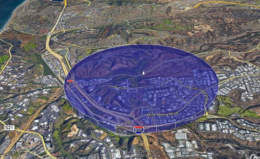
2 Field Trials

 This chapter presents results computed from data collected at our UAS Flight Center in San
 Diego, California.
 Flights were restricted to a cylindrical volume with 1.0 nautical mile radius and 400 ft altitude
 above ground level (AGL), as represented in Figure 2-1. This cylinder is centered at latitude
 32.904258, longitude -117.204767.
 All flights were performed in accordance with provisions in our certificate of authorization issued
 by the FAA.

 Figure 2-1 Flight test volume

 MAY CONTAIN U.S. AND INTERNATIONAL EXPORT CONTROLLED INFORMATION 9
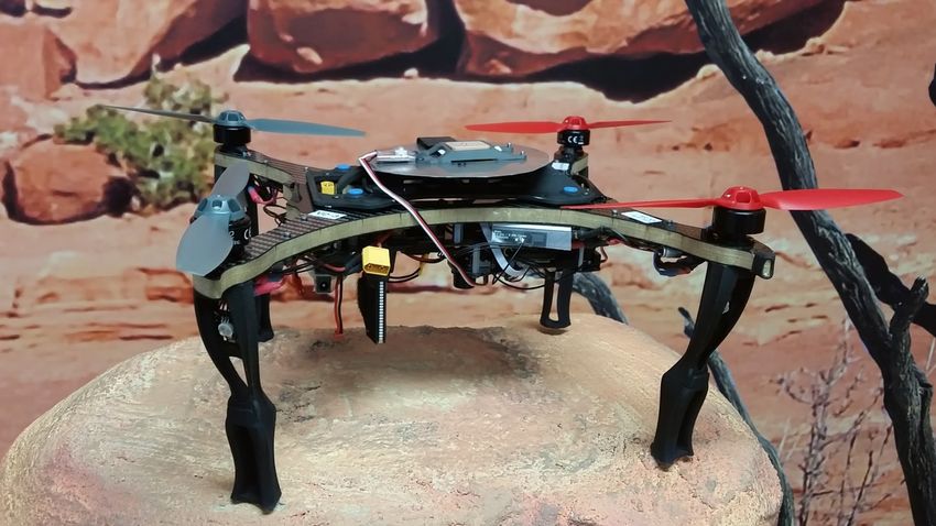
LTE Unmanned Aircraft Systems v1.0.1 Field Trials

 2.1 Measurement platform and data processing
 Flights and measurements for this phase of data collection were performed by a custom-designed
 quadrotor drone, the 390QC shown in Figure 2-2.
 The 390QC has a takeoff weight of 1050 grams and flight time of 16 minutes. It is equipped with
 the Qualcomm® Snapdragon Flight™ platform running Qualcomm® Snapdragon Navigator™
 flight control software.
 The drone executes fully autonomous data collection missions and can be monitored and
 controlled over Wi-Fi and/or LTE while in flight. An RC transmitter/receiver is active during all
 flights enabling immediate takeover from a ground operator for safety.

 Figure 2-2 390QC quadrotor drone

 The Snapdragon Flight platform connects to the LTE module capable of connecting in 700 MHz,
 AWS, and PCS bands.
 Rich LTE modem logs are collected simultaneously with Snapdragon Navigator logs enabling
 correlation of flight status and data with modem logs from synchronized timestamps. Logs are
 stored on an SD card on the drone, and transferred (either over network or by physically moving
 the SD card) to a database for long-term storage.

 MAY CONTAIN U.S. AND INTERNATIONAL EXPORT CONTROLLED INFORMATION 10
LTE Unmanned Aircraft Systems v1.0.1 Field Trials An analysis workstation is used to manipulate database records and to produce results in the form of statistics, plots, and maps as needed. This data pipeline is illustrated in Figure 2-3. antenna connectivity Snapdragon Modem diagnostic Flight logging Snapdragon modem Navigator logs logs (GPS, sensors, status, etc.) SDcard Results (statistics, Analysis plots, maps, etc.) SDcard Database Workstation Figure 2-3 Data pipeline 2.2 Summary of data sets For this trial, data was collected as indicated in Table 2-1. Table 2-1 Summary of data sets Data Description Location UAS Flight Center, San Diego, California Environment Mixed suburban Altitudes Ground, 30, 60, 90, 120 meters Test types Mobility route at 5 m/s with 0.5 Mbps UDP UL throughput requested Mobility route at 5 m/s and periodic RACH every 15 seconds Stop/Start route with 0.5 Mbps UDP UL throughput requested LTE bands (locked to PCS one band per flight) AWS 700 MHz Data collection On device logging (modem and Snapdragon Navigator logs). IPerf logs Connectivity was provided and tested using a commercial cellular network during all flights. For analysis of UL performance and interference, we employ a method of estimating the received energy as described in Section 2.4.2 and Appendix D. MAY CONTAIN U.S. AND INTERNATIONAL EXPORT CONTROLLED INFORMATION 11
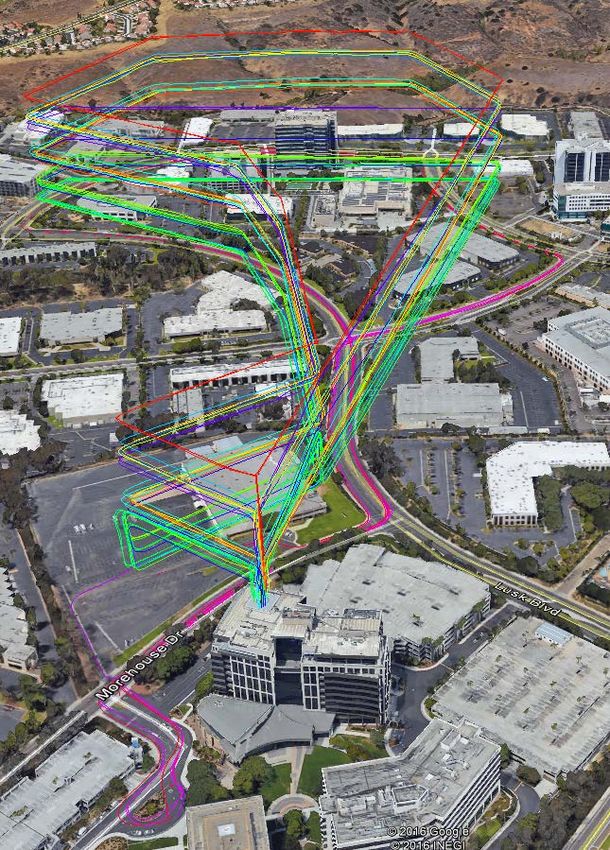
LTE Unmanned Aircraft Systems v1.0.1 Field Trials

 2.2.1 Mobility route
 Much of the analysis in later sections is derived from a 2.5 km loop as illustrated in Figure 2-4.
 The figure shows flights at different altitudes, and each altitude was flown multiple times for data
 collection in each band, and to provide sufficient data for each case (at least two loops).
 Table 2-2 lists the band and altitude permutations and the total duration for each case.
 The ground data was collected by mounting the drone to a car and driving the route on surface
 streets (the duration of these tests tended to be a bit longer than flying due to some stoplights and
 traffic).
 While Figure 2-4 shows flight traces including takeoff and landing from our rooftop helipad, each
 data set was trimmed so the final data for analysis only includes samples where the drone is at its
 intended altitude and underway. This prevents takeoff and landing transition data, as well as data
 when the drone is stationary on the landing pad, from impacting the analysis results.

 NOTE: The 30 meter and 60 meter flights are slightly different from the 90 meter and 120 meter flights.
 The lower altitudes caused the drone to be obstructed by a high-rise building so we decided to fly
 in front of the building to maintain primary pilot line-of-sight visibility during those tests.

 MAY CONTAIN U.S. AND INTERNATIONAL EXPORT CONTROLLED INFORMATION 12
LTE Unmanned Aircraft Systems v1.0.1 Field Trials

 Figure 2-4 Mobility route data included in analysis

 MAY CONTAIN U.S. AND INTERNATIONAL EXPORT CONTROLLED INFORMATION 13
LTE Unmanned Aircraft Systems v1.0.1 Field Trials

 Table 2-2 Band, altitude, and duration
 Band Alt (m) Total Time (min:sec)
 PCS 0 21:36
 PCS 30 12:36
 PCS 60 12:33
 PCS 90 32:21
 PCS 120 33:12
 AWS 0 27:44
 AWS 30 12:31
 AWS 60 12:34
 AWS 90 22:52
 AWS 120 15:49
 700 MHz 0 34:50
 700 MHz 30 18:44
 700 MHz 60 12:36
 700 MHz 90 16:50
 700 MHz 120 15:47

 2.3 Downlink: Mobility route results

 2.3.1 Detected cells
 We will start by looking at the number of detected cells at different altitudes and for different
 bands and then look at the distances to the detected cells. These views of the data do not consider
 received power from the cells (this comes later), just detectability.
 Figure 2-5 shows a histogram of the number of simultaneously detected cells for each band and
 altitude. The modem at each sample point (at approximately 160 ms intervals) returns a set of
 detected cells with one labeled as the serving cell – this is what is meant by simultaneously
 detected.
 The overall trend is the number of detected cells increases with altitude as expected due to the
 longer propagation distance of signals in the free space environments as altitude goes up.
 However, the trend is not without exceptions. For example, the mean number of detected cells for
 the 700 MHz band at 30 m is slightly lower than at the ground.

 MAY CONTAIN U.S. AND INTERNATIONAL EXPORT CONTROLLED INFORMATION 14
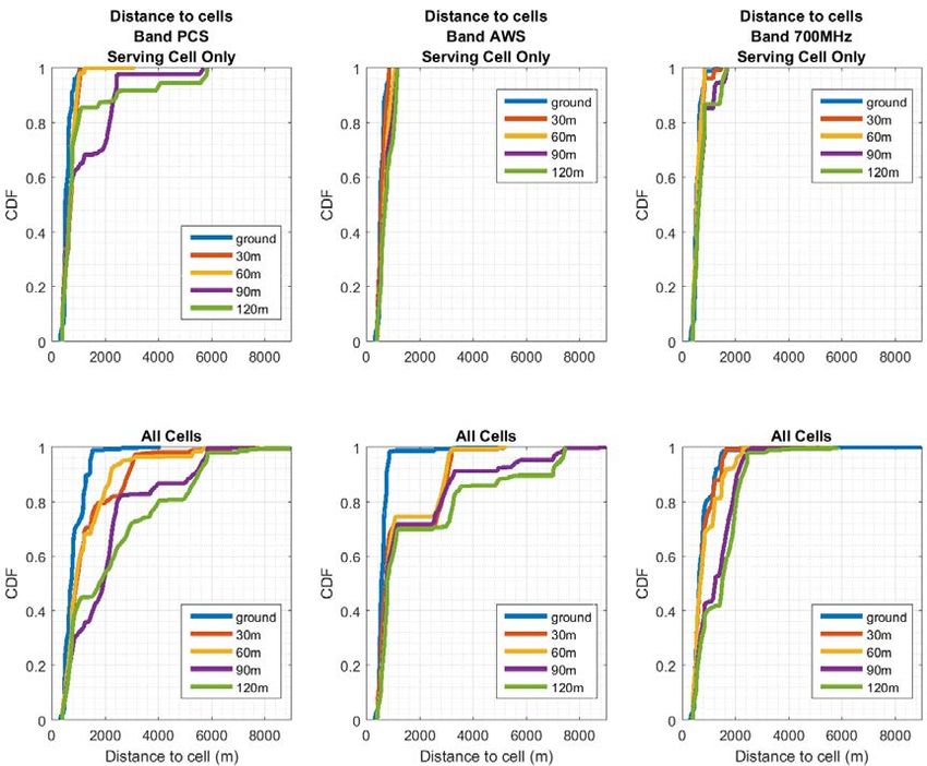
LTE Unmanned Aircraft Systems v1.0.1 Field Trials

 Figure 2-5 Histogram of simultaneously detected cell reference signals

 An alternate view of cell detectability is the distance distributions to detected cells. Here we
 consider all detections independently rather than grouping them by their detection instant.
 Figure 2-6 displays these distributions for each band. The top row of figures shows the serving
 cells only, and the bottom row considers all detected cells (including serving).
 Focusing first on the ground curves (in blue), all serving cells are within 1 km and virtually all
 neighbors within 2 km for all 3 bands. However, this changes significantly as we look at the
 nonground curves. Serving cell distance distributions for Bands AWS and 700 MHz are only
 mildly impacted by altitude, however PCS sees a more significant change. For example, >15% of
 PCS serving cells are at distance of > 5 km at 60 m altitude.
 Looking at all cells, altitude has a clear impact on the probability of detecting distant cells. It is
 surprising to see the impact appear much more severe for PCS than 700 MHz. AWS is in the

 MAY CONTAIN U.S. AND INTERNATIONAL EXPORT CONTROLLED INFORMATION 15
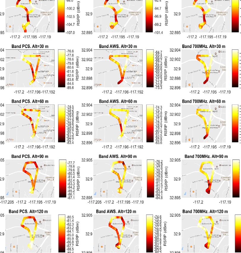
LTE Unmanned Aircraft Systems v1.0.1 Field Trials

 middle. The difference could be explained by the different numbers of cells in each band
 deployed in the test area.
 It is also counterintuitive that the data shows such longer distances to detectable PCS cells than
 700 MHz given that 700 MHz is expected to propagate further than PCS at 1900 MHz. PCS and
 700 MHz antennas are different with different pointing and different gain patterns, which are
 likely contributors to the observation of different detection distances.

 Figure 2-6 Distribution of distance to detected cells; top row includes only
 serving cells, bottom row adds all neighbor cells

 2.3.2 Serving cell analysis
 Now we take a closer look at serving cell data. The serving cell physical cell indicator (PCI),
 reference signal received power (RSRP) and reference signal received quality (RSRQ) are
 collected during test flights for each band and altitude combination. Depending on the band and
 altitude, we see as many as six serving cells and as few as one in a flight over the mobility route.
 In Figure 2-7, a representative flight was chosen for each band and altitude combination and the
 RSRPs are displayed. (While other flights do not show identical results, they are similar
 qualitatively to these). The RSRPs shown on the maps can be viewed using the color bars for
 each plot, where higher strength signals with larger RSRP are lighter in color, and lower strength
 signals are darker.

 MAY CONTAIN U.S. AND INTERNATIONAL EXPORT CONTROLLED INFORMATION 16
LTE Unmanned Aircraft Systems v1.0.1 Field Trials

 Figure 2-7 Maps of selected sample flights showing serving cell RSRP; the color
 bar scale is different for each map

 The distributions of the serving cell RSRP and RSRQ are shown in Figure 2-8 which allows a
 direct comparison across altitude and band. Ground RSRPs are lower than at altitude in general,
 though the high tail of the ground RSRP distribution shows the highest RSRPs of all. This is
 expected to be due to the higher chance of a ground user experiencing a direct line-of-sight
 directly into the main beam of the cell antenna. The fact that airborne users see stronger serving
 cell RSRPs than ground users has been surprising to some who expect the downtilted antennas to
 weaken signals significantly to airborne users. These results indicate that the stronger free space
 propagation to airborne users does in fact make up for antenna gain reductions.

 MAY CONTAIN U.S. AND INTERNATIONAL EXPORT CONTROLLED INFORMATION 17
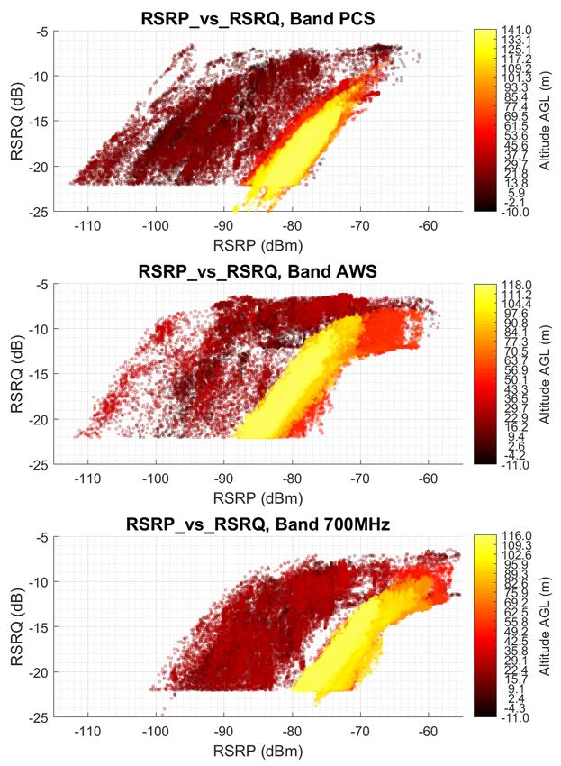
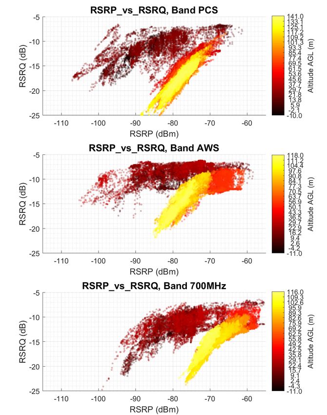
LTE Unmanned Aircraft Systems v1.0.1 Field Trials

 The RSRQ distributions however give an indication that interference grows with altitude until
 400 ft above ground. Median RSRQ reductions of 10 dB for the highest altitudes relative to
 ground are seen for Bands PCS and AWS and reductions of 4 dB for 700 MHz. The better
 relative RSRQ performance of 700 MHz may be due to the antenna downtilt and gain pattern
 difference across bands.

 Figure 2-8 Distributions of serving cell RSRP and RSRQ for each band and each
 altitude

 One way to visualize and analyze the simultaneous dependence of RSRP and RSRQ with altitude
 changes is using the scatter plots in Figure 2-9. Here, each point is a single sample with RSRP
 (dBm) on the x-axis, RSRQ (dB) on the y-axis, and colored with the altitude associated with the
 sample. Lighter colors represent higher altitude (see the color bar legends).
 In this visualization, the dependence becomes even clearer. Ground level samples cover a large
 range of RSRP and RSRQ. As altitude goes up, the range of values becomes tighter with
 generally stronger RSRP but depressed RSRQ. This behavior is similar for all three bands.

 MAY CONTAIN U.S. AND INTERNATIONAL EXPORT CONTROLLED INFORMATION 18
LTE Unmanned Aircraft Systems v1.0.1 Field Trials

 Figure 2-9 Scatterplots of serving cell RSRP vs. RSRQ for each band; points are
 colored by altitude (see color bar scale)

 MAY CONTAIN U.S. AND INTERNATIONAL EXPORT CONTROLLED INFORMATION 19
LTE Unmanned Aircraft Systems v1.0.1 Field Trials

 2.3.3 Neighbor cell analysis
 In this section, we expand to the analysis of neighbor cell detected signal characteristics. Because
 the relative strength between detected cells is an important factor for both handover algorithm
 performance and interference impact, we look at differences between detected signal RSRPs in
 dB.
 Figure 2-10 shows the distributions of the difference (Delta) between the serving cell RSRP and
 the nth strongest neighbor RSRP detected at the same instant.
 The first row of plots shows the first strongest neighbor, the second row shows the second
 strongest, third row the third strongest, and fourth row the fourth strongest neighbors. There is
 data for more neighbors, but it becomes less significant so we truncate the plots to the fourth
 strongest.
 Data for each band is shown in a separate plot as before. Thus, a point on the distribution
 represents the probability that at least the required number of neighbors is seen and the Delta
 RSRP is less than or equal to the value on the x-axis. The curves can be seen to plateau before
 reaching a probability of 1.0 due to the probability the nth neighbor is not detected at all.
 Note that negative Delta RSRP (RSRP inversion) values occur only when the serving cell is not
 the strongest cell. While this is not desirable in general, it often results even when the handover
 algorithm is fully optimized due to hysteresis parameters used to prevent rapid, or ping-pong
 handoff occurrence in the presence of highly dynamic signals particularly during mobility.
 Focusing first on the first strongest neighbor distributions, several points can be noted:
 ■ For all bands, the probability of RSRP inversion for ground tests is less than 10%, but as the
 altitude increases, this probability goes up.
 ■ Because handover trigger threshold is typically set to a small negative Delta RSRP (or RSRQ
 depending on the network configuration), higher probabilities of Delta RSRP in this range
 (say -3 dB to 0 dB) indicate a larger likelihood of interference and cell edge conditions during
 flights in the network at altitude than on the ground.
 For the second strongest neighbors, the ground data shows a negligible amount of energy for
 Bands AWS and 700 MHz and a small amount for PCS. However, as altitude increases, the
 contribution of the second strongest cell to interference becomes non-negligible. Similar
 conclusions are displayed for the third and fourth strongest.
 In studying this data, it is also clear that precise regularity in the results is not achieved, such as
 strictly monotonically increasing interference with altitude. For example, the distribution of
 second strongest interference for 700 MHz is noticeably higher at 90 m than for 120 m. We
 expect these kinds of results occur due to flights occurring in a limited geographical space in the
 network.

 MAY CONTAIN U.S. AND INTERNATIONAL EXPORT CONTROLLED INFORMATION 20
LTE Unmanned Aircraft Systems v1.0.1 Field Trials

 Figure 2-10 Distributions of DeltaRSRP (RSRPserving-RSRPneighbor,i)

 The results discussed rely on serving cell selection since the data are relative to serving cell
 RSRP, thus are impacted by the handover algorithm and its operational parameters.

 MAY CONTAIN U.S. AND INTERNATIONAL EXPORT CONTROLLED INFORMATION 21
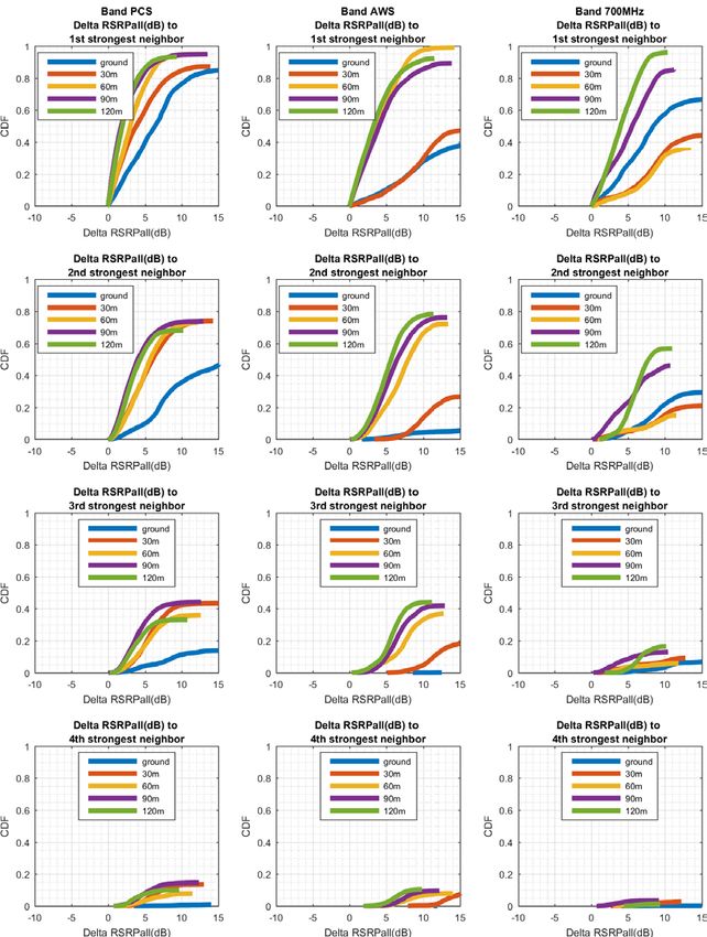
LTE Unmanned Aircraft Systems v1.0.1 Field Trials

 Figure 2-11 shows distributions of the same data, but using a slightly different metric we call
 Delta RSRPall. This metric computes the relative RSRP to the strongest cell always, and thus is
 independent of the serving cell selection (handover) algorithm. These distributions can be used to
 understand results based only on network layout and signal propagation. Note the Delta RSRPall
 metric is >0 by definition. We will not discuss these plots in detail here, and leave interpretation
 to the reader.
 Finally, the scatter plots in Figure 2-9 for serving cell measurements can be augmented to include
 all measurements (serving plus neighbor cells). This is shown in Figure 2-12. As can be seen, the
 overall character of the data is similar, but with many more sample points. The reported RSRQ
 has a lower limit of -22 dB, which is visible in the plots.

 MAY CONTAIN U.S. AND INTERNATIONAL EXPORT CONTROLLED INFORMATION 22
LTE Unmanned Aircraft Systems v1.0.1 Field Trials

 Figure 2-11 Distributions of Delta RSRPall

 MAY CONTAIN U.S. AND INTERNATIONAL EXPORT CONTROLLED INFORMATION 23
LTE Unmanned Aircraft Systems v1.0.1 Field Trials

 Figure 2-12 Scatterplots of RSRP vs. RSRQ for all detected cells for each band;
 points are colored by altitude (see color bar scale)

 MAY CONTAIN U.S. AND INTERNATIONAL EXPORT CONTROLLED INFORMATION 24
LTE Unmanned Aircraft Systems v1.0.1 Field Trials

 2.4 Uplink power and interference results

 2.4.1 Transmit power
 In this section, we discuss uplink results obtained from flights with a constant UL data stream of
 0.5 Mbps sent from the drone to our trial ground server.
 This is a relatively low data rate consistent with what would be required for a medium quality
 video stream. While future applications may demand higher rates, our intent here was to produce
 data enabling comparisons of performance across different altitudes without placing an undue
 burden on the commercial network during our trial flights. Tests of the limits of UL (and DL)
 throughput in flight are a suggested topic for future study.
 Total transmit power and the number of resource blocks (RBs) assigned as a function of time
 were logged during flights. This transmit power is determined by power control (Refer to
 Appendix C, 3GPP Technical Specification 36.213.)

 = min( , 10 10 ( ) + 0 + ∙ + ) (2-1)
 where
 = maximum power
 = number of RBs assigned
 0 = nominal value
 α = path loss scaling
 = estimated total (including antenna gains) path loss
 = accumulated closed-loop transmit power control (TPC) commands
 Figure 2-13 presents the distribution of transmit power per resource block (RB), 200 kHz per RB
 in the 700 MHz band. The larger path loss experienced on the ground causes larger transmit
 powers. Then the trend observed is that the transmit powers drop when in flight with narrowed
 distribution, but grow as the altitude of flight increases until about 400 ft above ground.

 Figure 2-13 Distribution of uplink transmit power density (per RB)

 MAY CONTAIN U.S. AND INTERNATIONAL EXPORT CONTROLLED INFORMATION 25
LTE Unmanned Aircraft Systems v1.0.1 Field Trials

 2.4.2 Estimated uplink interference
 While the transmit powers in flight are lower, we expect from the DL RSRP results that since
 differences between total path loss (TPL) of serving and neighbor cells are smaller in flight than
 on the ground, these transmissions arrive at the neighbor cells with relatively high power.
 Measuring these received powers at the cell is desirable, but due to the difficulty of attributing
 received energy to a single device in logging (at time of publication), this measurement was not
 available. However, it is possible to predict the received energy at a cell by assuming channel
 reciprocity between the DL and UL, and thus use the DL TPL estimate as an estimate of the
 UL TPL as well. This path loss can be estimated as

 = , − 10 10 (12 ∙ ) − (2-2)
 where
 , = total DL maximum transmit power for the cell
 = transmission bandwidth for the cell in RBs (eg. 50 for 10 MHz)
 = the measured RSRP at the device from this cell
 The second term simply scales down the total transmit power to the portion allocated to the
 reference signal.
 This method of estimating UL received energy is described further, including lab test validation,
 in Appendix D.
 Using this estimation of cell received power, we now look at distributions of power seen at
 neighbor cells. While the received power at the serving cell is carefully controlled for successful
 UL demodulation, the power at the neighbors is interference that impacts the overall uplink
 capacity of the network. Figure 2-14 shows distributions of received energy per RB across all
 neighbor cells detected in the trial data for 700MHz.
 The gap in these distributions across altitudes gives a statistical notion of the increase in
 interference produced. The gaps at the median are approximately 5 dB for 700MHz. This means a
 device at altitude can contribute 3 times the interference in the network in 700MHz than a ground
 user.
 Figure 2-15 shows a slightly altered view of this data. Here, the transmit powers per RB are
 scaled up to the power that would be seen if the drone had been utilizing all RBs in the system,
 but capping the maximum transmit power at 23 dBm. The distributions are similar, but clearly
 scaled up to full power. Also, the transmit power cap is seen to only influence the ground curve as
 this is much more likely to be impacted by transmit power cap.

 MAY CONTAIN U.S. AND INTERNATIONAL EXPORT CONTROLLED INFORMATION 26
LTE Unmanned Aircraft Systems v1.0.1 Field Trials

 Figure 2-14 Distributions of estimated uplink interference density at neighbor
 cells due to drone transmissions; interference is estimated assuming path loss
 measured on downlink is equivalent to uplink path loss for each cell

 Figure 2-15 Distributions of estimated total uplink interference at neighbor cells
 due to drone transmissions; here transmit power from drone is scaled up to the
 whole band (all RBs) subject to 23 dBm maximum transmit power

 MAY CONTAIN U.S. AND INTERNATIONAL EXPORT CONTROLLED INFORMATION 27
LTE Unmanned Aircraft Systems v1.0.1 Field Trials

 2.5 Handover analysis
 Handovers occurred during trial data collection a total of 206 times.
 Figure 2-16 shows distributions of the total interruption time during handovers. The majority of
 these are between 20-40 ms, but there are some outliers present as high as 800 ms. While these
 are not large interruption times, it is notable that the outliers are more likely in this data at
 altitudes 60 meters and higher.

 Figure 2-16 Handover events and distributions of delay in handover completion

 2.6 Path loss modeling
 Since it is expected that propagation differences at altitude relative to ground is one of the
 principal contributors to the different performance of the network for drones, we will look at path
 loss results from the field data.
 Here, path loss is considered to be only the over-the-air contribution without the effect of cell and
 drone antenna gain patterns. TPL or total path loss is the term used here when antenna effects are
 included, such as in Section 2.4. We use RS transmit power minus RSRP as the TPL (including
 antenna effects). Thus to study the over-the-air portion, it is necessary to estimate the antenna
 gain at both the transmitter and receiver and eliminate these from the total path loss measured.

 = , − 10 10 (12 ∙ ) − + + (2-3)
 where
 , = total DL maximum transmit power for the cell
 = transmission bandwidth for the cell in RBs (eg. 50 for 10 MHz)
 = the measured RSRP at the device from this cell
 = antenna gain at the drone
 = antenna gain at the cell

 MAY CONTAIN U.S. AND INTERNATIONAL EXPORT CONTROLLED INFORMATION 28
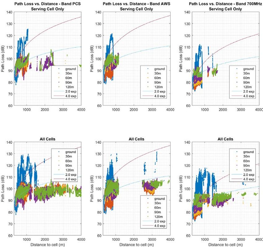
LTE Unmanned Aircraft Systems v1.0.1 Field Trials

 Antenna gains are obtained assuming a line-of-sight path from the cell antenna to the drone. This
 requires the relative positions of the cell and the drone to be known at all times, and the
 orientation (or attitude) of both the drone and the cell antennas are known in the global frame.
 Drone position and orientation (pitch, roll, and heading) are measured from the onboard flight
 controller, and cell antenna location and orientation (azimuth and downtilt) are known from a cell
 site database.
 The drone antenna pattern for each band was measured in an antenna chamber using the fully
 integrated drone package. These results are shown in Appendix E.1.
 The base station cell antenna gain patterns are obtained from manufacturer published patterns.
 We used unique patterns for each antenna type, frequency band, and electrical downtilt value. An
 example base station antenna pattern is shown in Appendix E.2.
 Results obtained using this technique are by nature approximate. We are using cell antenna
 patterns obtained during manufacturer testing in controlled environments, while the field
 measurements are obtained using antennas mounted in many different configurations and on
 different types of structures. The installed antenna patterns will be impacted by each particular
 installation. Further, direct line-of-sight is used for looking up the antenna gains, however
 reflected signals can have an important contribution to total power detected, especially for ground
 tests. Nevertheless, the analysis making these significant approximations is presented here as it
 still gives insight into the differences between propagation at different altitudes.
 Figure 2-17 shows these path loss samples as a function of distance from the drone to cell. Bands
 PCS, AWS, and 700MHz are plotted separately. The top row of plots shows serving cell samples
 only, and the bottom row adds neighbor cell samples. In addition to the sample point, analytical
 path loss models with exponent 2.0 and 4.0 are shown for reference given that those slopes are
 commonly used for free space and ground models respectively.
 One use of this type of analysis is guiding the path loss models for simulations. These results
 indicate the free space model (exponent 2.0) is a viable model to use for airborne vehicles in
 simulations. Here the free space model is

 4
 = 20 10 + 20 10
 (2-4)
 with d being distance in meters, f frequency in Hz, and c speed of light in m/s.

 MAY CONTAIN U.S. AND INTERNATIONAL EXPORT CONTROLLED INFORMATION 29
LTE Unmanned Aircraft Systems v1.0.1 Field Trials

 Figure 2-17 Path loss as a function of distance; top row is serving cell
 measurements only, bottom row adds neighbors

 MAY CONTAIN U.S. AND INTERNATIONAL EXPORT CONTROLLED INFORMATION 30
3 Simulations 3.1 Goals and scope The simulations performed for this trial were designed to study of performance tradeoffs when the network is serving many ground and airborne UEs simultaneously over a wide area. The simulations follow 3GPP system simulations guidelines for network layout and ground channel modeling. Here we present studies of: ■ Downlink SINR ■ Uplink interference and throughput ■ Mobility performance with airborne UEs in the network The goal is to give insights into the techniques that can be expected to provide the best payoff for overall performance of both ground and airborne UEs as the number of airborne UEs grows in the future. This also guides the plans and design of next-phase field trials to make sure such trials focus data collection and analysis on the most promising techniques. Note the simulation results are dependent on the evaluation methodologies including the network layout, propagation model and product implementations, and therefore should not be treated as the accurate absolute performance of actual networks. 3.2 Setup and assumptions The simulations performed used the setup described in Table 3-1. Table 3-1 Simulation setup Item Description Layout The layout follows the 3GPP D3 layout for system simulations in 3GPP Technical Specification 36.814 v9.0.0 (see Appendix C) with antennas modified for this simulation. The D3 layout is a hexagonal grid with 1732 meter site-to-site spacing, and 3 cells per site (pointed in 120 degrees azimuth increments). Due to the importance of the 3D antenna pattern for these simulations, the standard 3GPP simulation antenna was replaced with a 3D model of a representative commercial antenna, the 80010734_716MHz antenna (shown in Appendix E.2). Six degree mechanical downtilt was used for all antennas, and the total transmit power limit was set to 46 dBm. Band 700 MHz band only, with 10 MHz bandwidth MAY CONTAIN U.S. AND INTERNATIONAL EXPORT CONTROLLED INFORMATION 31
LTE Unmanned Aircraft Systems v1.0.1 Simulations Item Description Propagation Ground UEs are modeled using the 3GPP typical urban profile number 3 (TU3), modeling refer to Appendix C, 3GPP Technical Specification 36.814 v9.0.0. This model uses a path loss exponent of 3.76 and log-normal shadowing with standard deviation 8.0 dB. Drone UEs are all modeled with free space propagation and zero shadowing. This model uses a path loss exponent of 2.0. The explicit formula (in dB form) is provided in Section 2.6. 3.3 Downlink simulations Downlink results are captured by the SINR distribution computed in the simulation assuming full-buffer traffic. The simulator randomly and uniformly positions UEs in the network and then computes the received signal energy at each UE from all of the cells using the relevant propagation model and the cell parameters such as antenna gains and transmit power. Multiple samples are produced to randomize the UE locations in space and random model parameters such as log-normal shadowing. Then SINR is for a particular UE is = (3-1) +∑ =1 ≠ where is the signal power received from the jth cell. i is the index of the strongest signal (serving cell) and Mc is the number of cells. Thus, the SINR is the serving cell signal power divided by the sum of all other signal powers plus thermal noise, N. The received signal power is computed starting with the transmit power at the cell, applying the antenna gain (or attenuation) in the direction of the UE, and then applying the propagation losses from the propagation model relevant to that UE. For UEs at altitude, it is much more likely the strongest signal will come from outside the main beam of a cell than for UEs on the ground. This is the reason we used a commercial 3D antenna pattern that accurately models the gain in all directions for these simulations. This distribution gives a statistical picture of the signal quality that can be expected by users in the network. Since this distribution for users at one altitude is not affected by users at other altitudes, we perform these assumptions with all users at a single altitude, one altitude at a time. 3.3.1 Analysis of results Downlink SINR distributions from simulations of users at ground level, at 50 meters altitude, and at 120 meters altitude are shown in Figure 3-1. First we observe that the distribution for 50 meters and 120 meters are essentially identical. This indicates that, for this layout, the distribution is dominated by the propagation model differences between the ground and airborne UEs. We note a few key observations from these distributions: ■ SINRs are lower for airborne UEs, and this is expected due to the higher levels of interference from neighboring cells experienced due to the free space propagation of signals. The median degradation relative to ground users is approximately 5 dB. ■ The outage probability (defined here as SINR < -6 dB) from these simulation results is very similar for ground and airborne users, and is approximately 1%. DL spectral efficiency of MAY CONTAIN U.S. AND INTERNATIONAL EXPORT CONTROLLED INFORMATION 32
LTE Unmanned Aircraft Systems v1.0.1 Simulations

 140 kbps/MHz can be expected at -6 dB, and this would allow for 1.4 Mbps throughput given
 a 10 MHz allocation.
 1
 0.9
 0.8
 0.7
 0.6
 CDF

 0.5
 0.4
 0.3 Ground UEs
 0.2 Drones at 50m
 0.1 Drones at 120m
 0
 -10 -5 0 5 10 15 20 25 30 35 40
 DL SINR(dB)

 Figure 3-1 Distributions of downlink SINR for UEs at ground, 50 meter, and 120
 meter altitudes

 3.4 Uplink simulations
 Uplink simulations are performed to study the impact of altitude on interference levels at the cells
 and throughputs available to UEs.
 In contrast to full-buffer downlink simulations, uplink performance for a UE depends on the
 specific location (including altitude) and transmissions from neighboring UEs because they
 directly interfere with one another. Thus it no longer makes sense to simulate all UEs at a single
 altitude as we did for the downlink simulations. Here we fix the number of UEs per cell to 30,
 and perform simulations that vary the split of these users between ground level, and altitude. Here
 we selected 120 meters for all drone UEs.
 We focus on power control and resource partitioning as techniques for performance
 improvement. Some techniques require the network to distinguish between UEs at altitude and
 those on the ground to be effective, but other techniques can treat all UEs the same. Clearly it is
 simpler to use a method that does not require such UE identification, and we discuss this during
 the presentation of the results.
 We make use of the interference to thermal (IoT) ratio metric in these studies. This metric sums
 the contribution of received signal energy from all UEs served by neighboring cells and divides
 this by thermal noise. The plot axes are labeled preMMSEIoT to emphasize this metric is
 computed prior to the processing in the receive demodulator.
 Features are studied here without making reference to the precise feature design and
 configuration implemented in today’s networks. For example, there is no claim that the power
 control algorithms studied here are equivalent to the implementation in the commercial network
 studied in the Chapter 2 field trials. However, comparative study between algorithms can still be
 used to gauge the relative benefits of different approaches.

 MAY CONTAIN U.S. AND INTERNATIONAL EXPORT CONTROLLED INFORMATION 33
You can also read