Luxapose: Indoor Positioning with Mobile Phones and Visible Light
←
→
Page content transcription
If your browser does not render page correctly, please read the page content below
Luxapose:
   Indoor Positioning with Mobile Phones and Visible Light

                              Ye-Sheng Kuo, Pat Pannuto, Ko-Jen Hsiao, and Prabal Dutta
                                        Electrical Engineering and Computer Science Department
                                                          University of Michigan
                                                           Ann Arbor, MI 48109
                                        {samkuo,ppannuto,coolmark,prabal}@umich.edu

ABSTRACT                                                                       1.    INTRODUCTION
We explore the indoor positioning problem with unmodified smart-                    Accurate indoor positioning can enable a wide range of location-
phones and slightly-modified commercial LED luminaires. The                    based services across many sectors. Retailers, supermarkets, and
luminaires—modified to allow rapid, on-off keying—transmit their               shopping malls, for example, are interested in indoor positioning
identifiers and/or locations encoded in human-imperceptible optical            because it can provide improved navigation which helps avoid un-
pulses. A camera-equipped smartphone, using just a single image                realized sales when customers cannot find items they seek, and it
frame capture, can detect the presence of the luminaires in the image,         increases revenues from incremental sales from targeted advertis-
decode their transmitted identifiers and/or locations, and determine           ing [11]. Indeed, the desire to deploy indoor location-based services
the smartphone’s location and orientation relative to the luminaires.          is one reason that the overall demand for mobile indoor positioning
Continuous image capture and processing enables continuous posi-               in the retail sector is projected to grow to $5 billion by 2018 [7].
tion updates. The key insights underlying this work are (i) the driver         However, despite the strong demand forecast, indoor positioning
circuits of emerging LED lighting systems can be easily modified               remains a “grand challenge,” and no existing system offers accurate
to transmit data through on-off keying; (ii) the rolling shutter effect        location and orientation using unmodified smartphones [13].
of CMOS imagers can be leveraged to receive many bits of data                       WiFi and other RF-based approaches deliver accuracies mea-
encoded in the optical transmissions with just a single frame cap-             sured in meters and no orientation information, making them a poor
ture, (iii) a camera is intrinsically an angle-of-arrival sensor, so the       fit for many applications like retail navigation and shelf-level adver-
projection of multiple nearby light sources with known positions               tising [2, 5, 31]. Visible light-based approaches have shown some
onto a camera’s image plane can be framed as an instance of a                  promise for indoor positioning, but recent systems offer landmarks
sufficiently-constrained angle-of-arrival localization problem, and            with approximate room-level semantic localization [21], depend on
(iv) this problem can be solved with optimization techniques. We               custom hardware and received signal strength (RSS) techniques that
explore the feasibility of the design through an analytical model,             are difficult to calibrate, or require phone attachments and user-in-
demonstrate the viability of the design through a prototype system,            the-loop gestures [13]. These limitations make deploying indoor
discuss the challenges to a practical deployment including usability           positioning systems in “bring-your-own-device” environments, like
and scalability, and demonstrate decimeter-level accuracy in both              retail, difficult. Section 2 discusses these challenges in more de-
carefully controlled and more realistic human mobility scenarios.              tail noting, among other things, that visible light positioning (VLP)
                                                                               systems have demonstrated better performance than RF-based ones.
Categories and Subject Descriptors                                                  Motivated by a recent claim that “the most promising method
                                                                               for the new VLP systems is angle of arrival” [1], we propose a
B.4.2 [HARDWARE]: Input/Output and Data Communications—                        new approach to accurate indoor positioning that leverages trends
Input/Output Devices; C.3 [COMPUTER-COMMUNICATION                              in solid-state lighting, camera-enabled smartphones, and retailer-
NETWORKS]: Special-Purpose and Application-Based Systems                       specific mobile applications. Our design consists of visible light bea-
                                                                               cons, smartphones, and a cloud/cloudlet server that work together to
General Terms                                                                  determine a phone’s location and orientation, and support location-
Design, Experimentation, Measurement, Performance                              based services. Each beacon consists of a programmable oscillator
                                                                               or microcontroller that controls one or more LEDs in a luminaire.
                                                                               A beacon’s identity is encoded in the modulation frequency (or
Keywords                                                                       Manchester-encoded data stream) and optically broadcast by the
Indoor localization; Mobile phones; Angle-of-arrival; Image pro-               luminaire. The smartphone’s camera takes pictures periodically and
cessing                                                                        these pictures are processed to determine if they contain any beacons
                                                                               by testing for energy in a target spectrum of the columnar FFT of the
                                                                               image. If beacons are present, the images are decoded to determine
Permission to make digital or hard copies of part or all of this work is       the beacon location and identity. Once beacon identities and coor-
granted without fee provided that copies are not made or distributed for       dinates are determined, an angle-of-arrival localization algorithm
profit or commercial advantage and that copies bear this notice and the full   determines the phone’s absolute position and orientation in the local
citation on the first page.
                                                                               coordinate system. Section 3 presents an overview of our proposed
Copyright is held by the authors.                                              approach, including the system components, their interactions, and
MobiCom’14, September 7–11, 2014, Maui, HI, USA.                               the data processing pipeline that yields location and orientation from
ACM 978-1-4503-2783-1/14/09.                                                   a single image of the lights and access to a lookup table.
http://dx.doi.org/10.1145/2639108.2639109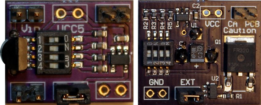
Our angle-of-arrival positioning principle assumes that three               Param        EZ       Radar    Horus     Epsilon    Luxapose
or more beacons (ideally at least four) with known 3-D coordi-               Reference        [5]        [2]     [31]      [13]        [this]
nates have been detected and located in an image captured by a                Position      2-7 m      3-5 m    ∼1 m      ∼0.4 m      ∼0.1 m
smartphone. We assume that these landmarks are visible and distin-           Orientation     n/a        n/a      n/a       n/a           3◦
guishable from each other. This is usually the case when the camera           Method        Model       FP       FP       Model        AoA
is in focus since unoccluded beacons that are separated in space              Database       Yes        Yes      Yes       No           Yes
uniquely project onto the camera imager at distinct points. Assum-
                                                                             Overhead        Low        WD      WD         DC           DC
ing that the camera geometry is known and the pixels onto which
the beacons are projected is determined, we estimate the position           Table 1: Comparison with prior WiFi- and VLC-based localization
and orientation of the smartphone with respect to the beacons’ co-          systems. FP, WD, AoA, and DC are FingerPrinting, War-Driving,
ordinate system through the geometry of similar triangles, using a          Angle-of-Arrival, and Device Configuration, respectively. These are
variation on the well-known bearings-only robot localization and            the reported figures from the cited works.
mapping problem [10]. Section 4 describes the details of estimating
position and orientation, and dealing with noisy measurements.
     So far, we have assumed that our positioning algorithm is given        2.    RELATED WORK
the identities and locations of beacons within an overhead scene
                                                                                 There are three areas of related work: RF localization, visible
image, but we have not discussed how are these extracted from an
                                                                            light communications, and visible light positioning.
image of modulated LEDs. Recall that the beacons are modulated
                                                                                 RF-Based Localization. The majority of indoor localization
with a square wave or transmit Manchester-encoded data (at frequen-
                                                                            research is RF-based, including WiFi [2, 5, 15, 27], Motes [14], and
cies above 1 kHz to avoid direct or indirect flicker [26]). When a
                                                                            FM radio [4], although some have explored magnetic fingerprinting
smartphone passes under a beacon, the beacon’s transmissions are
                                                                            as well [6]. All of these approaches achieve meter-level accuracy,
projected onto the camera. Although the beacon frequency far ex-
                                                                            and no orientation, often through RF received signal strength from
ceeds the camera’s frame rate, the transmissions are still decodable
                                                                            multiple beacons, or with location fingerprinting [4, 6, 14, 29]. Some
due to the rolling shutter effect [9]. CMOS imagers that employ a
                                                                            employ antenna arrays and track RF phase to achieve sub-meter
rolling shutter expose one or more columns at once, and scan just
                                                                            accuracy, but at the cost of substantial hardware modifications [27].
one column at a time. When an OOK-modulated light source illu-
                                                                            In contrast, we offer decimeter-level accuracy at the 90th-percentile
minates the camera, distinct light and dark bands appear in images.
                                                                            under typical overhead lighting conditions, provide orientation, use
The width of the bands depend on the scan time, and crucially, on
                                                                            camera-based localization, require no hardware modifications on
the frequency of the light. We employ an image processing pipeline,
                                                                            the phone and minor modifications to the lighting infrastructure.
as described in Section 5, to determine the extent of the beacons,
                                                                                 Visible Light Communications. A decade of VLC research
estimate their centroids, and extract their embedded frequencies,
                                                                            primarily has focused on high-speed data transfer using specialized
which yields the inputs needed for positioning.
                                                                            transmitters and receivers that support OOK, QAM, or DMT/OFDM
     To evaluate the viability and performance of this approach, we
                                                                            modulation [12], or the recently standardized IEEE 802.15.7 [22].
implement the proposed system using both custom and slightly-
                                                                            However, smartphones typically employ CdS photocells with wide
modified commercial LED luminaires, a Nokia Lumia 1020 smart-
                                                                            dynamic range but insufficient bandwidth for typical VLC [21].
phone, and an image processing pipeline implemented using OpenCV,
                                                                            In addition, CdS photocells cannot determine angle-of-arrival, and
as described in Section 6. We deploy our proof-of-concept system in
                                                                            while smartphone cameras can, they cannot support most VLC tech-
a university lab and find that under controlled settings with the smart-
                                                                            niques due to their limited frame rates. Recent research has shown
phone positioned under the luminaires, we achieve decimeter-level
                                                                            that by exploiting the rolling shutter effect of CMOS cameras, it is
location and roughly 3◦ orientation error under lights when four
                                                                            possible to receive OOK data at close range, from a single transmit-
or five beacons are visible. With fewer than four visible beacons,
                                                                            ter, with low background noise [9]. We also use the same effect but
or when errors are introduced in the beacon positions, we find that
                                                                            operate at 2-3 meter range from typical luminaires, support multiple
localization errors increase substantially. Fortunately, in realistic us-
                                                                            concurrent transmitters, and operate with ambient lighting levels.
age conditions—a person carrying a smartphone beneath overhead
                                                                                 Visible Light-Based Localization. Visible light positioning us-
lights—we observe decimeter position and single-digit orientation
                                                                            ing one [19,30,32] or more [20,28] image sensors has been studied in
errors. Although difficult to directly compare different systems, we
                                                                            simulation. In contrast, we explore the performance of a real system
adopt the parameters proposed by Epsilon [13] and compare the
                                                                            using a CMOS camera present in a commercial smartphone, address
performance of our system to the results reported in prior work in
                                                                            many practical concerns like dimming and flicker, and employ robust
Table 1. These results, and others benchmarking the performance of
                                                                            decoding and localization methods that work in practice. Several
the VLC channel, are presented in Section 7.
                                                                            visible light positioning systems have been implemented [13, 21, 24].
     Our proposed system, while promising, also has a number of
                                                                            ALTAIR uses ceiling-mounted cameras, body-worn IR LED tags,
limitations. It requires a high density of overhead lights with known
                                                                            and a server that instructs tags to beacon sequentially, captures im-
positions, and nearby beacons to have accurate relative positions.
                                                                            ages from the cameras, and performs triangulation to estimate po-
Adequate performance requires high-resolution cameras which have
                                                                            sition [24]. Epsilon uses LED beacons and a custom light sensor
only recently become available on smartphones. We currently up-
                                                                            that plugs into a smartphone’s audio port, and sometimes requires
load entire images to the cloud/cloudlet server for processing, which
                                                                            users to perform gestures [13]. The LEDs transmit data using BFSK
incurs a significant time and energy cost that is difficult to accu-
                                                                            and avoid persistent collisions by random channel hopping. The
rately characterize. However, we show simple smartphone-based
                                                                            system offers half-meter accuracy. In contrast, we require no custom
algorithms that can filter images locally, or crop only the promising
                                                                            hardware on the phone, can support a high density of lights without
parts of an image, reducing transfer costs or even enabling local
                                                                            coordination, require no special gestures, provide orientation, and
processing. Section 8 discusses these and other issues, and suggests
                                                                            typically offer better performance. Landmarks provides semantic
that it may soon be possible to achieve accurate indoor positioning
                                                                            (e.g. room-level) localization using rolling shutter-based VLC [21],
using unmodified smartphones in realistic retail settings.
                                                                            but neither accurate position nor orientation, like our system does.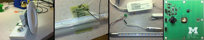
C C Image
freq location
Control
C C Plane
Unit
f1 (x1, y1, z1) Transmitters
§ 6.1
f2 (x2, y2, z2) T0 (x0, y0, z0)T Zf
f3 (x3, y3, z3) § 7.3
f4 (x4, y4, z4) Images
f1 f2 f3 f4 T 1 (x1, y 1, z 1 )T
i2 (a2, b2, Zf)R
§ 5.1, 5.4
Axis α α
i1 (a1, b1, Zf)R
§ 6.2 Take a picture § 5.1 i0 (a0, b0, Zf)R
(optional)
T2
§ 5.2 Beacon
location
Frequency
detection
§ 5.3
Cloud / (x2, y2, z2)T
§ 6.3 Cloudlet
§ 4.1, 4.2 AoA AoA
§ 4.3 Biconvex Lens
localization orientation
Figure 2: Optical AoA localization. When the scene is in focus, trans-
Location based
services § 7.2 mitters are distinctly projected onto the image plane. Knowing the
transmitters’ locations Tj (xj , yj , zj )T in a global reference frame,
Figure 1: Luxapose indoor positioning system architecture and and their image ij (aj , bj , Zf )R in the receiver’s reference frame,
roadmap to the paper. The system consists of visible light beacons, allows us to estimate the receiver’s global location and orientation.
mobile phones, and a cloud/cloudlet server. Beacons transmit their
identities or coordinates using human-imperceptible visible light. A
phone receives these transmissions using its camera and recruits a 4.1 Optical Angle-of-Arrival Localization
combination of local and cloud resources to determine its precise Luxapose uses optical angle-of-arrival (AoA) localization prin-
location and orientation relative to the beacons’ coordinate system ciples based on an ideal camera with a biconvex lens. An important
using an angle-of-arrival localization algorithm, thereby enabling property of a simple biconvex lens is that a ray of light that passes
location-based services. through the center of the lens is not refracted, as shown in Figure 2.
Thus, a transmitter, the center of the lens, and the projection of trans-
mitter onto the camera imager plane form a straight line. Assume
3. SYSTEM OVERVIEW that transmitter T0 , with coordinates (x0 , y0 , z0 )T in the transmit-
The Luxapose indoor positioning system consists of visible ters’ global frame of reference, has an image i0 , with coordinates
light beacons, smartphones, and a cloud/cloudlet server, as Figure 1 (a0 , b0 , Zf )R in the receiver’s frame of reference (with the origin
shows. These elements work together to determine a smartphone’s located at the center of the lens). T0 ’s position falls on the line
location and orientation, and support location-based services. Each that passes through (0, 0, 0)R and (a0 , b0 , Zf )R , where Zf is the
beacon consists of a programmable oscillator or microcontroller that distance from lens to imager in pixels. By the geometry of similar
modulates one or more LED lights in a light fixture to broadcast the triangles, we can define an unknown scaling factor K0 for transmit-
beacon’s identity and/or coordinates. The front-facing camera in a ter T0 , and describe T0 ’s location (u0 , v0 , w0 )R in the receiver’s
hand-held smartphone takes pictures periodically. These pictures are frame of reference as:
processed to determine if they contain LED beacons by testing for
the presence of certain frequencies. If beacons are likely present, the u0 = K0 × a0
images are decoded to both determine the beacon locations in the v0 = K0 × b0
image itself and to also extract data encoded in the beacons’ mod- w0 = K0 × Zf
ulated transmissions. A lookup table may be consulted to convert
beacon identities into corresponding coordinates if these data are not Our positioning algorithm assumes that transmitter locations
transmitted. Once beacon identities and coordinates are determined, are known. This allows us to express the pairwise distance be-
an angle-of-arrival localization algorithm determines the phone’s tween transmitters in both the transmitters’ and receiver’s frames
position and orientation in the venue’s coordinate system. This data of reference. Equating the expressions in the two different domains
can then be used for a range of location-based services. Cloud or yields a set of quadratic equations in which the only remaining
cloudlet resources may be used to assist with image processing, unknowns are the scaling factors K0 , K1 , . . . , Kn . For example, as-
coordinate lookup, database lookups, indoor navigation, dynamic sume three transmitters T0 , T1 , and T2 are at locations (x0 , y0 , z0 )T ,
advertisements, or other services that require distributed resources. (x1 , y1 , z1 )T , and (x2 , y2 , z2 )T , respectively. The pairwise distance
squared between T0 and T1 , denoted d20,1 , can be expressed in both
4. POSITIONING PRINCIPLES domains, and equated as follows:
Our goal is to estimate the location and orientation of a smart- d20,1 = (u0 − u1 )2 + (v0 − v1 )2 + (w0 − w1 )2
phone assuming that we know bearings to three or more point-
= (K0 a0 − K1 a1 )2 + (K0 b0 − K1 b1 )2 + Zf2 (K0 − K1 )2
sources (interchangeably called beacons, landmarks, and transmit-
ters) with known 3-D coordinates. We assume the landmarks are −−→2 −
−→2 −
−→ − −→
= K02 Oi0 + K12 Oi1 − 2K0 K1 (Oi0 · Oi1 )
visible and distinguishable from each other using a smartphone’s
built-in camera (or receiver). The camera is in focus so these point = (x0 − x1 )2 + (y0 − y1 )2 + (z0 − z1 )2 ,
sources uniquely project onto the camera imager at distinct pixel −−→ − −→
locations. Assuming that the camera geometry (e.g. pixel size, fo- where Oi0 and Oi1 are the vectors from the center of the lens to
cal length, etc.) is known and the pixels onto which the landmarks image i0 (a0 , b0 , Zf ) and i1 (a1 , b1 , Zf ), respectively. The only
are projected can be determined, we seek to estimate the position unknowns are K0 and K1 . Three transmitters would yield three
and orientation of the mobile device with respect to the landmarks’ quadratic equations in three unknown variables, allowing us to find
coordinate system. This problem is a variation on the well-known K0 , K1 , and K2 , and compute the transmitters’ locations in the
bearings-only robot localization and mapping problem [10]. receiver’s frame of reference.
y' y where the column vectors − →
r1 , −
→
r2 and −
→
r3 are the components of the
0 0 0
unit vectors x̂ , ŷ , and ẑ , respectively, projected onto the x, y, and
z axes in the transmitters’ frame of reference. Figure 3 illustrates the
relationships between these various vectors. Once the orientation
→
[]
| |
r1,x of the receiver is known, determining its bearing requires adjusting
→
r1 = r→ for portrait or landscape mode usage, and computing the projection
| |
1,y
→ onto the xy-plane.
→
r1,y
x̂'
| |
r1,z
→ →
z'
r1,z r1,x
x'
5. CAMCOM PHOTOGRAMMETRY
z x Our positioning scheme requires that we identify the points in a
camera image, (ai , bi , Zf ), onto which each landmark i ∈ 1 . . . N
Figure 3: Receiver orientation. The vectors x0 , y 0 , and z 0 are defined with known coordinates, (xi , yi , zi ), are projected, and map between
as shown in the picture. The projection of the unit vectors x̂0 , ŷ 0 , and the two domains. This requires us to: (i) identify landmarks in an
ẑ 0 onto the x, y, and z axes in the transmitters’ frame of reference image, (ii) label each landmark with an identity, and (iii) map that
give the elements of the rotation matrix R. identity to the landmark’s global coordinates. To help with this
process, we modify overhead LED luminaires so that they beacon
optically—by rapidly switching on and off—in a manner that is
4.2 Estimating Receiver Position imperceptible to humans but detectable by a smartphone camera.
In the previous section, we show how the transmitters’ locations We label each landmark by either modulating the landmark’s
in the receiver’s frame of reference can be calculated. In practice, LED at a fixed frequency or by transmitting Manchester-encoded
imperfections in the optics and inaccuracies in estimating the trans- data in the landmark’s transmissions (an approach called camera
mitters’ image locations make closed-form solutions unrealistic. To communications, or CamCom, that enables low data rate, unidirec-
address these issues, and to leverage additional transmitters beyond tional message broadcasts from LEDs to image sensors), as Sec-
the minimum needed, we frame position estimation as an optimiza- tion 5.1 describes. We detect the presence and estimate the centroids
tion problem that seeks the minimum mean square error (MMSE) and extent of landmarks in an image using the image processing
over a set of scaling factors, as follows: pipeline described in Section 5.2. Once the landmarks are found, we
−1 determine their identities by decoding data embedded in the image,
2 −−→ −−→ −−→ −−→
NP N 2 2
+ Kn2 Oin − 2Km Kn (Oim · Oin ) − d2mn }2 ,
P
{Km Oim which either contains an index to, or the actual value of, a landmark’s
m=1 n=m+1
coordinates, as described in Section 5.3. Finally, we estimate the
where N is the number of transmitters projected onto the image, capacity of the CamCom channel we employ in Section 5.4.
resulting in N2 equations.
Once all the scaling factors are estimated, the transmitters’ loca- 5.1 Encoding Data in Landmark Beacons
tions can be determined in the receiver’s frame of reference, and the Our system employs a unidirectional communications channel
distances between the receiver and transmitters can be calculated. that uses an LED as a transmitter and a smartphone camera as a
The relationship between two domains can be expressed as follows: receiver. We encode data by modulating signals on the LED trans-
mitter. As our LEDs are used to illuminate the environment, it is
x0 x1 . . . xN −1 u0 u1 . . . uN −1 important that our system generates neither direct nor indirect flicker
y0 y1 . . . yN −1 = R × v0 v1 . . . vN −1 + T,
(the stroboscopic effect). The Lighting Research Center found that
z0 y1 . . . zN −1 w0 w1 . . . wN −1 for any duty cycle, a luminaire with a flicker rate over 1 kHz was ac-
ceptable to room occupants, who could perceive neither effect [26].
where R is a 3-by-3 rotation matrix and T is a 3-by-1 translation
matrix. 5.1.1 Camera Communications Channel
The elements of T (Tx , Ty , Tz ) represent the receiver’s location When capturing an image, most CMOS imagers expose one or
in the transmitters’ frame of reference. We determine the translation more columns of pixels, but read out only one column at a time,
matrix based on geometric relationships. Since scaling factors are sweeping across the image at a fixed scan rate to create a rolling
now known, equivalent distances in both domains allow us to obtain shutter, as shown in Figure 4a. When a rapidly modulated LED is
the receiver’s location in the transmitters’ coordinate system: captured with a CMOS imager, the result is a banding effect in the
(Tx − xm )2 + (Ty − ym )2 + (Tz − zm )2 = Km
2
(a2m + b2m + Zf2 ), image in which some columns capture the LED when it is on and
others when it is off. This effect is neither visible to the naked eye,
where (xm , ym , zm ) are the coordinates of the m-th transmitter in nor in a photograph that uses an auto-exposure setting, as shown
the transmitters’ frame of reference, and (am , bm ) is the projection in Figure 4b. However, the rolling shutter effect is visible when an
of the m-th transmitter onto the image plane. Finally, we estimate image is captured using a short exposure time, as seen in Figure 4c.
the receiver’s location by finding the set (Tx , Ty , Tz ) that minimizes: In the Luxapose design, each LED transmits a single frequency
N (from roughly 25-30 choices) as Figure 4c shows, allowing different
{(Tx − xm )2 + (Ty − ym )2 + (Tz − zm )2 − Km
2
(a2m + b2m + Zf2 )}2
P
m=1 LEDs or LED constellations to be distinctly identified. To expand
the capacity of this channel, we also explore Manchester encoded
4.3 Estimating Receiver Orientation data transmission, which is appealing both for its simplicity and its
Once the translation matrix T is known, we can find the rotation absence of a DC-component, which supports our data-independent
matrix R by individually finding each element in it. The 3-by-3 brightness constraint. Figure 4d shows an image captured by an
rotation matrix R is represented using three column vectors, −
→
r1 , −
→
r2 , unmodified Lumia 1020 phone 1 m away from a commercial 6 inch
−
→
and r3 , as follows: can light. Our goal is to illustrate the basic viability of sending
information over our VLC channel, but leave to future work the
R= −
h
→
r1 − →
r2 − →
i
r3 , problem of determining the optimal channel coding.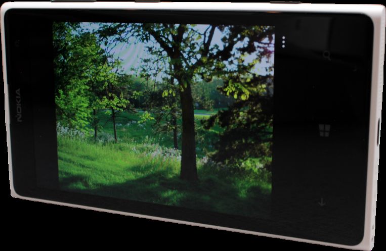
LED ON OFF ON
n-1 n n+1
pixel "n" pixel "n"
Column start exposing end exposing
exposure
timing pixel "n"
read out
Image
time
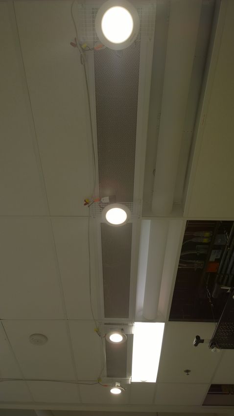
(a) Banding pattern due to the rolling (b) Auto Exposure. Image of (c) Pure Tone. Image of an (d) Manchester Encoding. (e) Hybrid Encoding. Im-
shutter effect of a CMOS camera cap- an LED modulated at 1 kHz LED modulated at 1 kHz Image of an LED modu- age of an LED alternat-
turing a rapidly flashing LED. Ad- with a 50% duty-cycle taken with a 50% duty-cycle taken lated at 1 kHz with a 50% ing between transmitting a
justing the LED frequency or duty with the built-in camera app with a short exposure setting. duty-cycle transmitting 3 kHz Manchester encoded
cycle changes the width of light and with a default (auto) expo- The modulation is clearly vis- Manchester-encoded data data stream and a 6 kHz pure
dark bands in the image, allowing fre- sure settings. The modula- ible as a series of alternating taken with a short exposure tone. Data is 4 symbols and
quency to be detected and decoded. tion is imperceptible. light and dark bands. setting. Data repeats 0x66. the preamble is 2 symbols.
Figure 4: CMOS rolling shutter principles and practice using various encoding schemes. All images are taken by a Lumia 1020 camera of a
modified Commercial Electric T66 6 inch (10 cm) ceiling-mounted can LED. The camera is 1 m from the LED and pictures are taken with the
back camera. The images shown are a 600 × 600 pixel crop focusing on the transmitter, yielding a transmitter image with about a 450 pixel
diameter. The ambient lighting conditions are held constant across all images, demonstrating the importance of exposure control for CamCom.
5.1.2 Camera Control
Relative amplitude
250
Cameras export many properties that affect how they capture 200
images. The two most significant for the receiver in our CamCom 150
channel are exposure time and film speed. 100
Exposure Control. Exposure time determines how long each 50
pixel collects photons. During exposure, a pixel’s charge accumu- 0
1/16667 1/8000 1/6410 1/5000 1/4000 1/3205
lates as light strikes, until the pixel saturates. We seek to maximize
Exposure time
the relative amplitude between the on and off bands in the captured
image. Figure 5 shows the relative amplitude across a range of ex- ISO 100 ISO 400 ISO 3200
posure values. We find that independent of film speed (ISO setting),
the best performance is achieved with the shortest exposure time. Figure 5: Maximizing SNR, or the ratio between the brightest and
The direct ray of light from the transmitter is strong and requires less darkest pixels in an image. The longer the exposure, the higher the
than an on-period of the transmitted signal to saturate a pixel. For a probability that a pixel accumulates charge while another saturates,
1 kHz signal (0.5 ms on, 0.5 ms off), an exposure time of longer than reducing the resulting contrast between the light and dark bands. As
0.5 ms (1/2000 s) guarantees that each pixel will be at least partially film speed (ISO) increases, a fewer number of photons are required
exposed to an on period, which would reduce possible contrast and to saturate each pixel. Hence, we minimize the exposure time and
result in poorer discrimination between light and dark bands. film speed to maximize the contrast ratio, improving SNR.
Film Speed. Film speed (ISO setting) determines the sensitivity
or gain of the image sensor. Loosely, it is a measure of how many
photons are required to saturate a pixel. A faster film speed (higher
ISO) increases the gain of the pixel sense circuitry, causing each 5.3 Decoding Data in Images
pixel to saturate with fewer photons. If the received signal has a low Once the centroid and extent of any landmarks are found in
amplitude (far from the transmitter or low transmit power), a faster an image, the next step is to extract the data encoded in beacon
film speed could help enhance the image contrast and potentially transmissions in these regions using one of four methods.
enlarge the decoding area. It also introduces the possibility of am- Decoding Pure Tones – Method One. Our first method of fre-
plifying unwanted reflections above the noise floor, however. As quency decoding samples the center row of pixels across an image
Figure 5 shows, a higher film speed increases the importance of a subregion and takes an FFT of that vector. While this approach de-
shorter exposure time for high contrast images. We prefer smaller codes accurately, we find that it is not very precise, requiring roughly
ISO values due to the proximity and brightness of indoor lights. 200 Hz of separation between adjacent frequencies to reliably de-
code. We find in our evaluation, however, that this approach decodes
more quickly and over longer distances than method two, creating a
5.2 Finding Landmarks in an Image tradeoff space, and potential optimization opportunities.
Independent of any modulated data, the first step is to find the Decoding Pure Tones – Method Two. Figures 6g to 6j show
centroid and size of each transmitter on the captured image. We our second method, an image processing approach. We first apply
present one method in Figures 6a to 6e for identifying disjoint, circu- a vertical blur to the subregion and then use an OTSU filter to get
lar transmitters (e.g. individual light fixtures). We convert the image threshold values to pass into the Canny edge detection algorithm [3].
to grayscale, blur it, and pass it through a binary OTSU filter [18]. Note the extreme pixelation seen on the edges drawn in Figure 6i;
We find contours for each blob [25] and then find the minimum these edges are only 1 pixel wide. The transmitter captured in this
enclosing circle (or other shape) for each contour. After finding each subregion has a radius of only 35 pixels. To manage this quantization,
of the transmitters, we examine each subregion of the image inde- we exploit the noisy nature of the detected vertical edge and compute
pendently to decode data from each light. We discuss approaches the weighted average of the edge location estimate across each row,
for processing other fixture types, such as Figure 18, in Section 8. yielding a subpixel estimation of the column containing the edge.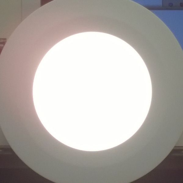
(a) Original (Cropped)             (b) Blurred             (c) Binary OTSU [18]          (d) Contours [25]           (e) Result: Centers

   (f) Subregion (131×131 px)         (g) Vertical Blur         (h) ToZero OTSU [18]         (i) Canny Edges [3]         (j) Result: Frequency
Figure 6: Image processing pipeline. The top row of images illustrate our landmark detection algorithm. The bottom row of images illustrate
our image processing pipeline for frequency recovery. These images are edited to move the transmitters closer together for presentation.

     Near the transmitter center, erroneous edges are sometimes iden-        5.4       Estimating Channel Capacity
tified if the intensity of an on band changes too quickly. We majority           The size of the transmitter and its distance from the receiver
vote across three rows of the subregion (the three rows equally parti-       dictate the area that the transmitter projects onto the imager plane.
tion the subregion) to decide if each interval is light or dark. If an       The bandwidth for a specific transmitter is determined by its image
edge creates two successive light intervals, it is considered an error       length (in pixels) along the CMOS scan direction. Assuming a
and removed. Using these precise edge estimates and the known                circular transmitter with diameter A m, its length on the image
scan rate, we convert the interval distance in pixels to the transmitted     sensor is A × f /h pixels, where f is the focal length of the camera
frequency with a precision of about 50 Hz., offering roughly 120             and h is the height from the transmitter to the receiver. The field of
channels (6 kHz/50 Hz). In addition to the extra edge detection and          view (FoV) of a camera can be expressed as α = 2 × arctan( 2×f   X
                                                                                                                                                  ),
removal we also attempt to detect and insert missing edges. We               where X is the length of the image sensor along the direction of the
compute the interval values between each pair of edges and look for          FoV. Combining these, the length of the projected transmitter can
intervals that are statistical outliers. If the projected frequency from                             A×X
                                                                             be expressed as h×2×tan(F           .
                                                                                                          oV /2)
the non-outlying edges divides cleanly into the outlier interval, then           As an example, in a typical retail setting, A is 0.3~0.5 m and
we have likely identified a missing edge, and so we add it.                  h is 3~5 m. The Glass camera (X = 2528 px, 14.7° FoV) has a
     Decoding Manchester Data. To decode Manchester data, we                 “bandwidth” of 588~1633 px. The higher-resolution Lumia 1020
use a more signal processing-oriented approach. Like the FFT for             camera (X = 5360 px, 37.4° FoV) bandwidth is actually lower,
tone, we operate on only the center row of pixels from the subre-            475~1320 px, as the wider FoV maps a much larger scene area to
gion. We use a matched filter with a known pattern (a preamble)              the fixed-size imager as the distance increases. This result shows
at different frequencies and search for the maximum correlation.             that increasing resolution alone may not increase effective channel
When found, the maximum correlation also reveals the preamble                capacity without paying attention to other camera properties.
location. The frequency of the matched filter is determined by the
                                                              Fs
number of pixels per symbol. It can be calculated as 2×n         , where
Fs is the sampling rate of the camera and n is an integer. As the            6.    IMPLEMENTATION DETAILS
frequency increases, n decreases, and the quantization effect grows.              To evaluate the viability and performance of the Luxapose de-
For example, Fs on the Lumia 1020 is 47.54 kHz, so an n value of             sign, we implement a prototype system using a variety of LED
5 matches a 4.75 kHz signal. Using the best discrete matched filter,         luminaires, an unmodified smartphone, and a Python-based cloudlet
we search for the highest correlation value anywhere along the real          (all available at https://github.com/lab11/vlc-localization/).
pixel x-axis, allowing for a subpixel estimation of symbol location,
repeating this process for each symbol.                                      6.1       LED Landmarks
     Decoding Hybrid Transmissions. To balance the reliability of                 We construct landmarks by modifying commercial LED lumi-
detecting pure tones with the advantages of Manchester encoded               naires, including can, tube, and task lamps, as shown in Figure 7a,
data, we explore a hybrid approach, alternating the transmission of          but full-custom designs are also possible. Figure 7b shows the mod-
a pure tone and Manchester encoded data, as Figure 4e shows. By              ifications, which include cutting (×) and intercepting a wire, and
combining frequency and data transmission, we decouple localiza-             wiring in a control unit that includes a voltage regulator (VR) and a
tion from communication. When a receiver is near a transmitter, it           microcontroller (MCU) or programmable oscillator (OSC) control-
can take advantage of the available data channel, but it can also de-        ling a single FET switch. We implement two control units, as shown
code the frequency information of lights that are far away, increasing       in Figure 7c, for low- and high-voltage LED driver circuits, using a
the probability of a successful localization.                                voltage-controlled oscillator with 16 frequency settings.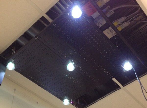
(a) LED landmarks: can, tube, task, and custom beacons.

120                        MCU
         AC / DC    VR      or

VAC     converter          OSC.

                                                                            Figure 8: Indoor positioning testbed. Five LED beacons are mounted
                    Control Unit
                                     (c) Programmable control units.
                                                                            246 cm above the ground for experiments. Ground truth is provided
  (b) Luminaire modifications.                                              by a pegboard on the floor with 2.54 cm location resolution.
Figure 7: LED landmarks. (a) Commercial and custom LED beacons.
(b) A commercial luminaire is modified by inserting a control unit.
(c) Two custom control units with 16 programmable tones. The units          we move an object from the center to the edge of the camera’s
draw 5 mA and cost ~$3 each in quantities of 1,000, suggesting they         frame, and find that the Lumia’s images show very little distortion,
could be integrated into commercial luminaires.                             deviating at most 3 pixels from the expected location.
                                                                                The distance, Zf , between the center of lens and the imager is a
                                                                            very important parameter in AoA localization algorithms. Unfortu-
                                                                            nately, this parameter is not fixed on the Lumia 1020, which uses a
6.2     Smartphone Receiver                                                 motor to adjust the lens for sharper images. This raises the question
     We use the Nokia Lumia 1020 to implement the Luxapose re-              of how this impacts localization accuracy. In a simple biconvex lens
ceiver design. The Lumia’s resolution—7712×5360 pixels—is the               model, the relationship between s1 (distance from object to lens),
highest among many popular phones, allowing us the greatest exper-          s2 (from lens to image), and f (focal length) is:
imental flexibility. The deciding factor, however, is not the hardware                                 1    1    1
capability of the smartphone, but rather its OS support and camera                                        +    =
                                                                                                       s1   s2   f
API that expose control of resolution, exposure time, and film speed.
Neither Apple’s iOS nor Google’s Android currently provide the                  where s2 and Zf are the same parameter but s2 is measured in
needed camera control, but we believe they are forthcoming. Only            meters whereas Zf is measured in pixels. s2 can be rewritten as
                                                                            s1 ×f
Windows Phone 8, which runs on the Lumia, currently provides a              s1 −f
                                                                                  . For the Lumia 1020, f = 7.2 mm. In the general use case, s1
rich enough API to perform advanced photography [16].                       is on the order of meters which leads to s2 values between 7.25 mm
     We modify the Nokia Camera Explorer [17] to build our applica-         (s1 = 1 m) and 7.2 mm (s1 = ∞). This suggests that Zf should
tion. We augment the app to expose the full range of resolution and         deviate only 0.7% from a 1 m focus to infinity. As lighting fixtures
exposure settings, and we add a streaming picture mode that continu-        are most likely 2∼5 m above ground, the practical deviation is even
ously takes images as fast as the hardware will allow. Finally, we add      smaller, thus we elect to use a fixed Zf value for localization. We
cloud integration, transferring captured images to our local cloudlet       measure Zf while the camera focuses at 2.45 m across 3 Lumia
for processing, storage, and visualization without employing any            phones. All Zf values fall within 0.15% of the average: 5,620 pixels.
smartphone-based optimizations that would filter images.                        While the front camera is more likely to face lights in day-to-
     We emphasize that the platform support is not a hardware issue         day use, we use the back camera for our experiments since it offers
but a software issue. Exposure and ISO settings are controlled by           higher resolution. Both cameras support the same exposure and ISO
OS-managed feedback loops. We are able to coerce these feedback             ranges, but have different resolutions and scan rates. Scan rate places
loops by shining a bright light into imagers and removing it at the         an upper bound on transmit frequency, but the limited exposure
last moment before capturing an image of our transmitters. Using            range places a more restrictive bound, making this difference moot.
this technique, we are able to capture images with 1/7519 s exposure        Resolution imposes an actual limit by causing quantization effects
on ISO 68 film using Google Glass and 1/55556 s exposure and ISO 50         to occur at lower frequencies; the maximum frequency decodable
on an iPhone 5; we are able to recover the location information from        by the front camera using edge detection is ∼5 kHz, while the
these coerced-exposure images successfully, but evaluating using            back camera can reach ∼7 kHz. Given Hendy’s Law—the annual
this approach is impractical, so we focus our efforts on the Lumia.         doubling of pixels per dollar—we focus our evaluation on the higher-
     Photogrammetry—the discipline of making measurements from              resolution imager, without loss of generality.
photographs—requires camera characterization and calibration. We
use the Nokia Pro Camera application included with the Lumia,               6.3     Cloudlet Server
which allows the user to specify exposure and ISO settings, to cap-             A cloudlet server implements the full image processing pipeline
ture images for this purpose. Using known phone locations, beacon           shown in Figure 6 using OpenCV 2.4.8 with Python bindings. On
locations, and beacon frequencies, we measure the distance between          an unburdened MacBook Pro with a 2.7 GHz Core i7, the median
the lens and imager, Zf (1039 pixels, 5620 pixels), and scan rate           processing time for the full 33 MP images captured by the Lumia
(30,880 columns/s, 47,540 columns/s), for the front and back cameras, re-   is about 9 s (taking picture: 4.46 s, upload: 3.41 s, image process-
spectively. To estimate the impact of manufacturing tolerances, we          ing: 0.3 s, estimate location: 0.87 s) without any optimizations. The
measure these parameters across several Lumia 1020s and find only a         cloudlet application contains a mapping from transmitter frequency
0.15% deviation, suggesting that per-unit calibration is not required.      to absolute transmitter position in space. Using this mapping and
     Camera optics can distort a captured image, but most smartphone        the information from the image processing, we implement the tech-
cameras digitally correct distortions in the camera firmware [23]. To       niques described in Section 4 using the leastsq implementation
verify the presence and quality of distortion correction in the Lumia,      from SciPy. Our complete cloudlet application is 722 Python SLOC.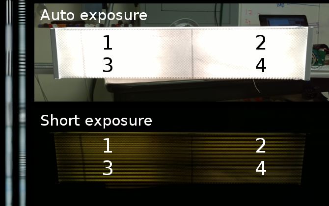
-60 -60 -60
TX 4 TX 3 TX 4 TX 3
-40 -40 -40
-20 -20 -20
0 0 0
y
y
y
Walking path
Walking path TX 5 TX 5
20 20 20
40 40 40
TX 1 TX 2 TX 1 TX 2
60 60 60
180 160 140 120 100 -100 -80 -60 -40 -20 0 20 40 60 80 100 -60 -40 -20 0 20 40 60
z x x
Location Orientation Location Orientation Location Orientation
(a) YZ view (back) (b) XY view (top) (c) Model train moving at 6.75 cm/s
1
80 -60
0.9
TX 4 TX 3
0.8 100 -40
0.7
120 -20
0.6
CDF
0.5 140 0
z
y
Walking path
TX 5
0.4
160 20
0.3
0.2 180 40
TX 1 TX 2
0.1 200 60
0
1 10 100 -100 -80 -60 -40 -20 0 20 40 60 80 100 -60 -40 -20 0 20 40 60
Location/Angular error (cm/degree) x x
Under(Location) Under(Angular)
Outside(Location) Outside(Angular) Location Orientation Location Orientation
(d) CDF of location and angular error (e) XZ view (side) (f) Model train moving at 13.5 cm/s
Figure 9: Key location and orientation results under realistic usage conditions on our indoor positioning testbed. The shaded areas are directly
under the lights. (a), (b), and (e) show Luxapose’s estimated location and orientation of a person walking from the back, top, and side views,
respectively, while using the system. A subject carrying a phone walks underneath the testbed repeatedly, trying to remain approximately
under the center (x = −100 . . . 100, y = 0, z = 140). We measure the walking speed at ~1 m/s. (d) suggests location estimates (solid line) and
orientation (dotted line) under the lights (blue), have lower error than outside the lights (red). (c) and (f) show the effect of motion blur. To
estimate the impact of motion while capturing images, we place the smartphone on a model train running in an oval at two speeds. While the
exact ground truth for each point is unknown, we find the majority of the estimates fall close to the track and point as expected.
7. EVALUATION 7.2 Realistic Positioning Performance
In this section, we evaluate position and orientation accuracy in To evaluate the positioning accuracy of the Luxapose system
both typical usage conditions and in carefully controlled settings. under realistic usage conditions, we perform an experiment in which
We also evaluate the visible light communications channel for pure a person repeatedly walks under the indoor positioning testbed,
tones, Manchester-encoded data, and a hybrid of the two. Our exper- from left to right at 1 m/s, as shown from the top view of the testbed
iments are carried out on a custom indoor positioning testbed. in Figure 9b and side view in Figure 9e. The CDF of estimated loca-
tion and orientation errors when the subject is under the landmarks
7.1 Experimental Methodology (shaded) or outside the landmarks (unshaded) is shown in Figure 9d.
We integrate five LED landmarks, a smartphone, and a cloudlet When under the landmarks, our results show a median location error
server into an indoor positioning testbed, as Figure 8 shows. The of 7 cm and orientation error of 6◦ , substantially better than when
LED landmarks are mounted on a height-adjustable pegboard and outside the landmarks, which exhibit substantially higher magnitude
they form a 71.1×73.7 cm rectangle with a center point. A com- (and somewhat symmetric) location and orientation errors.
plementary pegboard is affixed to floor and aligned using a laser To evaluate the effect of controlled turning while under the
sight and verified with a plumb-bob, creating a 3D grid with 2.54 cm landmarks, we place a phone on a model train running at 6.75 cm/s
resolution of known locations for our experimental evaluation. To in an oval, as shown in Figure 9c. Most of the location samples fall
isolate localization from communications performance, we set the on or within 10 cm of the track with the notable exception of when
transmitters to emit pure tones in the range of 2 kHz to 4 kHz, the phone is collinear with three of the transmitters, where the error
with 500 Hz separation, which ensures reliable communications increases to about 30 cm, though this is an artifact of the localization
(we also test communications performance separately). Using this methodology and not the motion. When the speed of the train is
testbed, we evaluate indoor positioning accuracy—both location and doubled—to 13.5 cm/s—we find a visible increase in location and
orientation—for a person, model train, and statically. orientation errors, as shown in Figure 9f.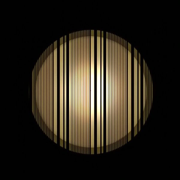
1
0.9
-49.5 -49.5 0.8 Precise TXs
140 140
0.7 1 TX with 5% err
Location (cm)
Location (cm)
120 120
TX 4 TX 3 TX 4 TX 3
0.6
CDF
TX 5 100 100 0.5 2 TXs with 5% err
80 80 0.4 3 TXs with 5% err
60 60 0.3 4 TXs with 5% err
TX 1 TX 2 40 TX 1 40 0.2
20 20 0.1 5 TXs with 5% err
52.1 0 52.1 0
0
0 10 20 30 40 50 60 70 80
-50.8 0 50.8 -50.8 0 50.8
Location (cm) Location (cm) Error (cm)
Figure 11: CDF of location error from a 5% error in absolute trans-
(a) Heat map with 5 TXs. (b) Heat map W/O TX 2,5. mitter location under the same conditions as Figure 10a. This exper-
1 1 iment simulates the effect of installation errors.
0.9 0.9
0.8 0.8
0.7 0.7
3
0.6 0.6
2
CDF
CDF
0.5 0.5 All TXs present
1
0.4 0.4 W/O TX 1
0
W/O TX 5 0 50 100 150 200 250 300 350
0.3 0.3
W/O TX 2, 3
0.2 0.2
W/O TX 2, 4 Z’-Axis rotation
Angle error (°)
0.1 0.1
All TXs present W/O TX 2, 5
0 0 3
0 20 40 60 80 100 120 140 0 20 40 60 80 100 120 140 2
Error (cm) Error (cm) 1
0
(c) CDF with all TXs present. (d) CDFs when TXs removed. -30 -20 -10 0 10 20 30
Figure 10: Localization accuracy at a fixed height (246 cm). (a) Y’-Axis rotation
3
shows a heat map of error when all 5 transmitters are present in 2
the image, and (c) shows a CDF of the error. (d) explores how 1
the system degrades as transmitters are removed. Removing any 0
-20 -15 -10 -5 0 5 10 15 20
one transmitter (corner or center) has minimal impact on location
error, still remaining within 10 cm for ~90% of locations. Removing X’-Axis rotation
Angle (°)
two transmitters (leaving only the minimum number of transmitters)
raises error to 20~60 cm when corners are lost and as high as 120 cm Figure 12: We rotate the mobile phone along axes parallel to the z 0 -,
when the center and a corner are lost. As shown in the heat map in y 0 -, and x0 -axis. Along the z 0 -axis, the mobile phone rotates 45° at a
(b), removing the center and corner generates the greatest errors as time and covers a full circle. Because of FoV constraints, the y 0 -axis
it creates sample points with both the largest minimum distance to rotation is limited to -27° to 27° and the x0 -axis is limited to -18° to
any transmitter and the largest mean distance to all transmitters. 18° with 9° increments. The experiments are conducted at a height
of 240 cm. The angle error for all measurements falls within 3°.
7.3 Controlled Positioning Accuracy Thus far, we have assumed the precise location of each transmit-
To evaluate the limits of positioning accuracy under controlled, ters is known. Figure 11 explores the effect of transmitter installation
static conditions, we take 81 pictures in a grid pattern across 100 × error on positioning by introducing a 5% error in 1–5 transmitter
100 cm area 246 cm below the transmitters and perform localization. positions and re-running the experiment from Figure 10a. With
When all five transmitters are active, the average position error across 5% error in the origin of all five transmitters, our system has only
all 81 locations is 7 cm, as shown in Figure 10a and Figure 10c. a 30 cm 50th percentile error, which suggests some tolerance to
Removing any one transmitter, corner or center, yields very similar installation-time measurement and calibration errors.
results to the five-transmitter case, as seen in the CDF in Figure 10d. To evaluate the orientation error from localization, we rotate
Removing two transmitters can be done in three ways: (i) remov- the phone along the x0 , y 0 , and z 0 axes. We compute the estimated
ing two opposite corners, (ii) removing two transmitters from the rotation using our localization system and compare it to ground
same side, and (iii) removing one corner and the center. Performing truth when the phone is placed 240 cm below the 5 transmitters.
localization requires three transmitters that form a triangle on the Figure 12 shows the orientation accuracy across all 3 rotation axes.
image plane, so (i) is not a viable option. Scenario (iii) introduces The rotation errors fall within 3° in all measurements.
the largest error, captured in the heatmap in Figure 10b, with an
average error as high as 50 cm in the corner underneath the missing 7.4 Frequency-Based Identification
transmitter. In the case of a missing side (ii), the area underneath the We evaluate two frequency decoders and find that the FFT is
missing transmitters has an average error of only 29 cm. Figure 10d more robust, but edge-detection gives better results when it succeeds.
summarizes the results of the removing various transmitter subsets. Rx Frequency Error vs Tx Frequency. Figure 13 sweeps the
In our worst case results, on an unmodified smartphone we are transmit frequency from 1 to 10 kHz in 500 Hz steps and evaluates
able to achieve parity (∼50 cm accuracy) with the results of systems the ability of both the FFT and edge detector to correctly identify
such as Epsilon [13] that require dedicated receiver hardware in the transmitted frequency. The edge detector with 1/16667 s exposure
addition to the infrastructure costs of a localization system. However, performs best until 7 kHz when the edges can no longer be detected
with only one additional transmitter in sight, we are able to achieve and it fails completely. The FFT detector cannot detect the frequency
an order of magnitude improvement in location accuracy. as precisely, but can decode a wider range of frequencies.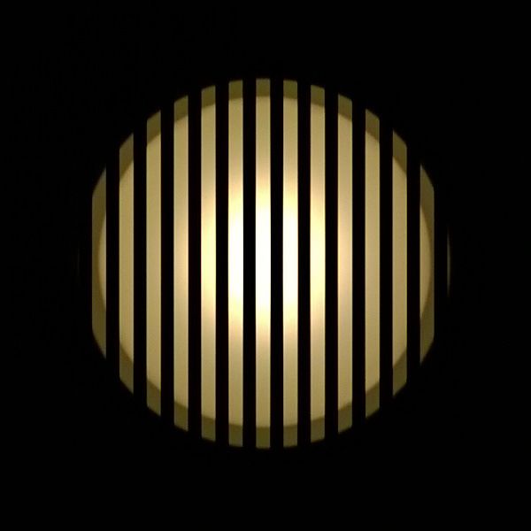
Proj. diameter(pixels)
100 100
Decoded freq. (Hz)
1100 160 5500
Measured 2.5 KHz
BW (symbols)
900 Calculated 3.5 KHz 10-1 10-1
120 4.5 KHz 4500
10-2 10-2
SER
SER
700 5.5 KHz
80 3500
500 6.5 KHz 10-3 10-3
300 40 10-4 2500 10-4
10-5 10-5
0.5 1 1.5 2 2.5 3 3.5 0.5 1 1.5 2 2.5 3 3.5 0.5 1 1.5 2 2.5 3 3.5 0.5 1 1.5 2 2.5 3 3.5 0.5 1 1.5 2 2.5 3 3.5
Distance (m) Distance (m) Distance (m) Distance (m) Distance (m)
(a) Transmitter length (b) Available bandwidth (c) SER (Known f.) (d) Frequency decoding (e) SER (Unknown f.)
Figure 15: Examining the decodability of Manchester data across various transmit frequencies and distances. Figures (b) through (e) share the
same legends. The transmitted frequencies are 2.5 KHz, 3.5 KHz, 4.5 KHz, 5.5 KHz and 6.5 KHz.
Dec. Rate (%)
3 3
RMS freq. error (Hz)
RMS freq. error (Hz)
10 10 1
0.75
102 102 0.5
0.25
101 101 0
0.5 1 1.5 2 2.5 3 3.5
100 100
1 2 3 4 5 6 7 8 9 10 1 2 3 4 5 6 7 8 9 10 Distance from transmitter (m)
Transmitted frequency (kHz) Transmitted frequency (kHz)
data length = 4 symbols
(a) Using edge detection (b) Using FFT data length = 8 symbols
Figure 13: Frequency recovery at 0.2 m, 1/16667 s, ISO 100. The edge Figure 16: Hybrid decoding is able to better tolerate the frequency
detector performs better until ∼7 kHz when quantization causes it quantization ambiguity than pure Manchester. Shorter data has a
to fail completely. The FFT method has lower resolution but can higher probability of being correctly decoded at long distances.
decode a wider frequency range.
300 300 7.5 Decoding Manchester Data
RMS freq. error (Hz)
RMS freq. error (Hz)
250 250 The relative size of a transmitter in a captured image dominates
200 200 data decodability. If the physical width of a transmitter is A and
150 150
the distance from the imager is D, the width of the transmitter on
100 100
50 50
the image is A/D × Zf pixels. Figure 15a shows measured width
0 0 in pixels and theoretical values at different distances. Figure 15b
0 1 2 3 4 5 6 0 1 2 3 4 5 6 shows the effect on the maximum theoretical bandwidth when using
Distance from transmitter(m) Distance from transmitter(m) Manchester encoding for various frequencies. Figure 15c finds that
ISO 100 ISO 800 ISO 100 ISO 800 if the transmitter frequency is known, the symbol error rate (SER) is
∼10−3 . Our sweeping match filter is able to detect frequency until a
(a) Using edge detection (b) Using FFT
quantization cutoff, as Figure 15d shows. When the frequency is not
Figure 14: As distance grows, the light intensity and area fall super- known a priori, Figure 15e shows that the SER correlates strongly
linearly. Using a higher ISO amplifies what little light is captured, with the ability to decode frequency.
enhancing frequency recoverability. We transmit a 1 kHz frequency
on a commercial LED and find that the decoded frequency error 7.6 Decoding Hybrid Data
remains under 100 Hz for distances up to 6 m from the transmitter. Hybrid decoding first decodes the pure tone frequency and then
is able to use the known frequency to improve its ability to decode
the data. As distance increases, the probability of capturing the data
Rx Frequency Error vs Tx Distance. As the distance between segment in the limited transmitter area falls, thus Figure 16 finds
the transmitter and phone increases, the received energy at each pixel that shorter messages are more robust to large distances.
drops due to line of sight path loss [8]. The area of the transmitter
projected onto the imager plane also decreases. These factors reduce
the ability to decode information. In Figure 14 we use a 10 cm 8. DISCUSSION
diameter 14 W Commercial Electric can light to explore the impact In this section, we discuss some limitations of our current system
of distance on our ability to recover frequency, and the effect of and potential directions for future work.
varying the ISO to attempt to compensate for the lower received Deployment Considerations. In real settings, all LED loca-
power. As intensity fades, the edge detection cannot reliably detect tions must be known, although only the relative distances between
edges and it fails. The FFT method is more robust to this failure, as closely located LEDs must be known with high accuracy. Although
it is able to better take advantage of pixels with medium intensity. not trivial, it does not seem difficult to ensure that this condition
The Importance of Frequency Channels. Human constraints holds. We have deployed a grid of sixteen luminaires in our lab,
and optics constraints limit our bandwidth to 1~7 kHz. With an and we analyze the effect of location errors on localization accuracy
effective resolution of 200 Hz, the FFT decoder can only identify in Section 7.3. We note that almost any localization system must
about 30 channels, and thus can only label 30 unique transmitters. know the anchor locations. In a practical setting, this would be done,
The finer 50 Hz resolution of the edge detector allows for about presumably, with the aid of blueprints and a laser rangefinder.
120 channels. A typical warehouse-style store, however, can easily Usability. Our system targets an active user, so that the front-
have over 1,000 lights. We explore techniques for more efficiently facing camera naturally observes the ceiling during use. Passive
using this limited set of frequency channels in Section 8. localization (e.g. while the phone is in a pocket) is out of scope.You can also read