Hirshfeld methods and Quantum Crystallography - M. Giorgi & A. van der Lee - cdifx
←
→
Page content transcription
If your browser does not render page correctly, please read the page content below
Hirshfeld methods and Quantum Crystallography

            Hirshfeld methods and Quantum Crystallography

                                        M. Giorgi & A. van der Lee

                           Fédération des sciences chimiques de Marseille, Marseille
                               Institut Européen des Membranes, Montpellier

AvdL
Hirshfeld methods and Quantum Crystallography
       Introduction

                              Quantum Crystallography ?

                                                   See also: Genoni et al., Quantum Crystallography:

                                                  Current developments and future perspectives, Chem.

                                                     Eur. J., 2018, DOI:10.1002/chem.201705952

AvdL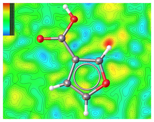
Hirshfeld methods and Quantum Crystallography
       Introduction

               QC results and XRD as mutual constraints

                                             Clinton et al. (1969)

                                       Jayatilaka & Dittrich (2008)
AvdL
Hirshfeld methods and Quantum Crystallography
       Introduction

                 Doing more with your diffraction data - I

                                          Tarahhomi & Van der Lee, in press (2018)

AvdL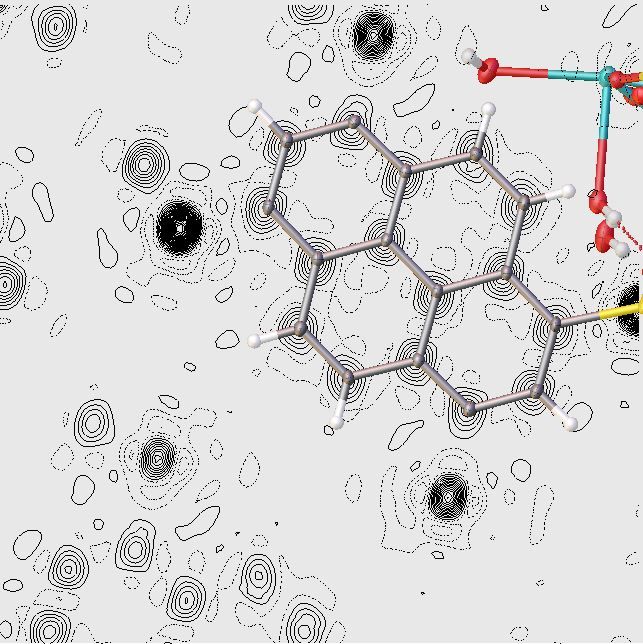
Hirshfeld methods and Quantum Crystallography
       Introduction

                 Doing more with your diffraction data - II

                            Classical and more advanced structure analyses
              I       Classical analysis
                        I   atomic positions → structure
                        I   packing features
                        I   interactions by analysis of atom-atom distances
              I       Electron density (ground state of the system - Hohenberg-Kohn
                      theorem)
                        I   → total energy of the system
                        I   → molecular properties such as inter and intramolecular
                            interactions/chemical bonds

                               ρ(r) is a quantum-mechanical observable!
AvdL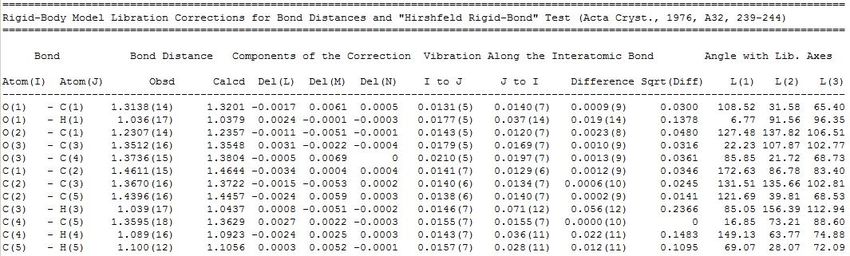
Hirshfeld methods and Quantum Crystallography
       Contents

                                                  Contents

                                          From theory to practice
              I   Electron density and chemical bonding
              I   Experimental and theoretical modelling of electron densities
              I   Hirshfeld analysis
                    I   Hirshfeld surfaces
                    I   Hirshfeld refinement
              I   Software
                    I   Tonto & CrystalExplorer
                    I   Tonto & OLEX2

AvdL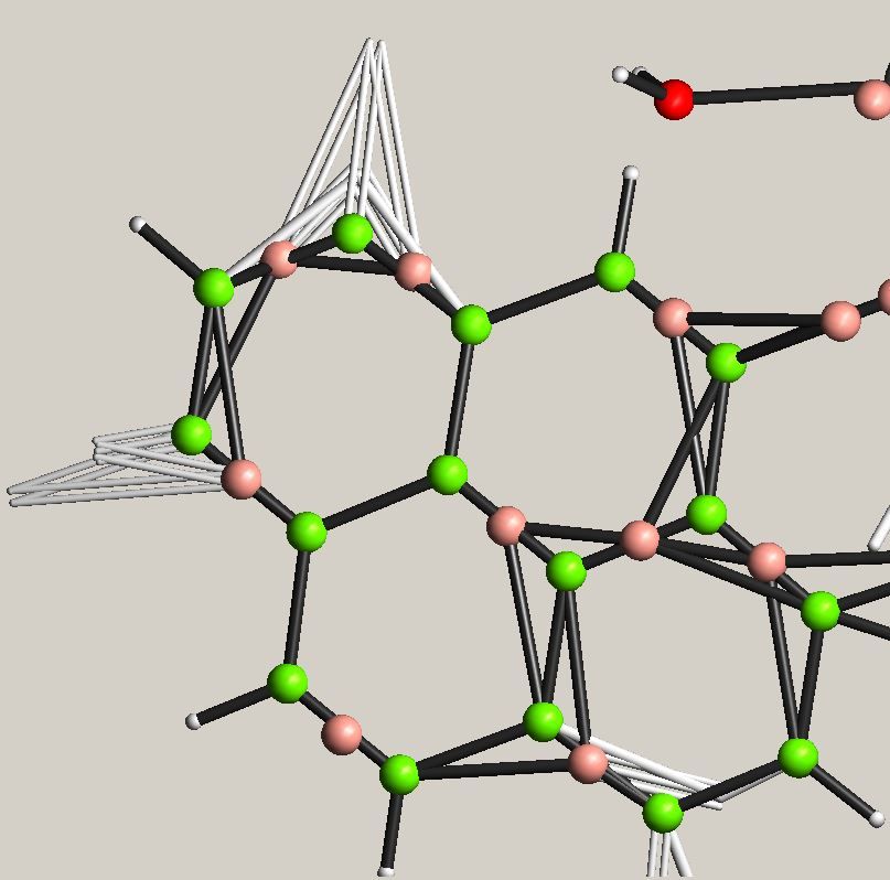
Hirshfeld methods and Quantum Crystallography
       Electron density and chemical bonding

                                                    Contents

                                               From theory to practice
              I     Electron density and chemical bonding
              I    Experimental and theoretical modelling of electron densities
              I    Hirshfeld analysis
                       I   Hirshfeld surfaces
                       I   Hirshfeld refinement
              I    Software
                       I   Tonto & CrystalExplorer
                       I   Tonto & OLEX2

AvdL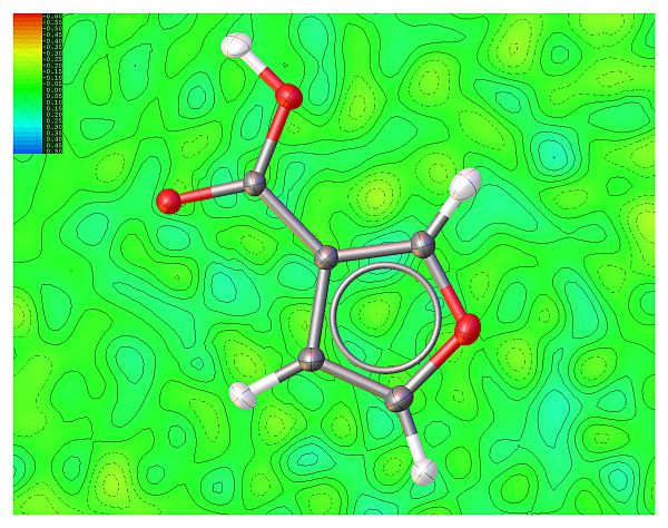
Hirshfeld methods and Quantum Crystallography
       Electron density and chemical bonding

                               X-rays interact with electrons

                           RECIPROCS BAG at Soleil - february 2018 - Zheng, Legrand, Van der Lee et al.

AvdL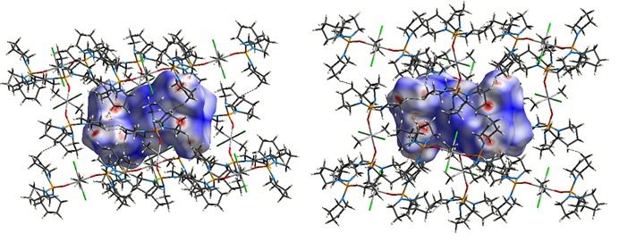
Hirshfeld methods and Quantum Crystallography
       Electron density and chemical bonding

                                               Residual density

                           RECIPROCS BAG at Soleil - february 2018 - Zheng, Legrand, Van der Lee et al.

AvdL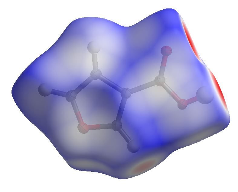
Hirshfeld methods and Quantum Crystallography
       Electron density and chemical bonding

                  History of electron density and chemical
                                 bonding - I

           It seems to me that the experimental study of scattered radiation,
           in particular from light atoms, should get more attention, since
           along this way it should be possible to determine the arrangement
           of the electrons in the atoms
           P. Debye - Zerstreuung von Röntgenstrahlen: Ann. Phys 351, 809-823
           (1915)

           An electron may form a part of the shell of two different atoms and
           cannot be said to belong to either one exclusively
           G. N. Lewis - The atoms and the molecule : J. Am. Chem. Soc. 38,
           762-785 (1916)

AvdL
Hirshfeld methods and Quantum Crystallography
Electron density and chemical bonding
History of electron density and chemical
bonding - II
Pauling (1939) - On the nature of the chemical bond →
application to the elucidation of complex substances
Bader (1965 - 1990) - Quantum theory of atoms in molecules →
chemical bonding based on the topology of electron density
distribution
Stewart (1976), Hansen & Coppens (1978) - Extension of
refinement techniques to include effects of chemical bonding
AvdLHirshfeld methods and Quantum Crystallography
Experimental and theoretical modelling of electron densities
Contents
From theory to practice
I Electron density and chemical bonding
I Experimental and theoretical modelling of electron densities
I Hirshfeld analysis
I Hirshfeld surfaces
I Hirshfeld refinement
I Software
I Tonto & CrystalExplorer
I Tonto & OLEX2Hirshfeld methods and Quantum Crystallography
Experimental and theoretical modelling of electron densities
Experimental determination of electron
density
AvdLHirshfeld methods and Quantum Crystallography
Experimental and theoretical modelling of electron densities
The spherical and the aspherical model
X
F (hkl) = fj exp[2πi(hxj + yj + zj )]
j
Z
fj (q, E ) = ρj (r ) exp[iq.r ]d 3 r
spherical electron distribution →
Z
fj (q, E ) = ρj (r ) exp[iq.r ]d 3 r
IAM: Independent Atom Model
AvdLHirshfeld methods and Quantum Crystallography
Experimental and theoretical modelling of electron densities
Calculation of spherical atomic scattering
factors
IAM uses quantum-mechanically calculated atomic scattering
factors (ex-situ) · · · as does Hirshfeld Atomic Refinement (in-situ).
AvdLHirshfeld methods and Quantum Crystallography
Experimental and theoretical modelling of electron densities
Treatment of the aspherical atomic scattering
factors in the multipole model
atoms N
NX X sym h
F (q) = Pi,core fi,core (q) + Pi,val fi,val (q, κ)+
i j
4 l i
Φil (q, κ0l )
X X
i
Pilm Ylm (q/|q|) e iq.rij .Ti (q)
l m=−l
Three contributions: core - spherical valence - aspherical valence
electrons; fi,core and fi,val are derived from the classical spherical
atomic scattering factors f (q, E )
To be refined: population parameters P, expansion-contraction
parameters κ and κ0Hirshfeld methods and Quantum Crystallography
Experimental and theoretical modelling of electron densities
In between the IAM and the multipole model
The different single-crystal refinement methods
I Independent atom model refinements (SHELXL, CRYSTALS,
JANA)
I Intermediate approaches
I Maximum Entropy methods (BAYMEM)
I Database transfer (INVARIOM, MOPRO)
I Hirshfeld refinement (TONTO)
I Multipole refinements (XD, MOPRO, JANA)Hirshfeld methods and Quantum Crystallography
Experimental and theoretical modelling of electron densities
Quantum-mechanical determination of
electron density
Solve the Schrödinger equation
Ĥψ = E ψ
Two approaches
I Wave function based ab initio → ρ is the square of the
absolute value of the wave function
I Electron density based → density functional treatment
AvdLHirshfeld methods and Quantum Crystallography
Hirshfeld analysis
Hirshfeld surfaces
Contents
From theory to practice
I Electron density and chemical bonding
I Experimental and theoretical modelling of electron densities
I Hirshfeld analysis
I Hirshfeld surfaces
I Hirshfeld refinement
I Software
I Tonto & CrystalExplorer
I Tonto & OLEX2Hirshfeld methods and Quantum Crystallography
Hirshfeld analysis
Hirshfeld surfaces
The Hirshfeld surface
Where are the interactions between molecules located in space?
How is the surface of a molecule defined?
→ Hirshfeld partitioning:
PNmolecule
ρi (r) ρpromolecule (r)
w (r) = Pi=1
Ncrystal
=
ρi (r) ρprocrystal (r)
i=1
where ρi (r) is the spherically-averaged atomic electron density
function.
Hirshfeld surface → w (r) = 1/2
AvdLHirshfeld methods and Quantum Crystallography
Hirshfeld analysis
Hirshfeld surfaces
Intermezzo
Hirshfeld did not invent the Hirshfeld surface, but he did invent the
’stockholder partitioning scheme’ for an atom in a molecule;
Spackman generalized the concept to a molecule in a crystal and
named it Hirshfeld surface.
AvdLHirshfeld methods and Quantum Crystallography
Hirshfeld analysis
Hirshfeld surfaces
The Hirshfeld atom
ρi (r) ρi (r)
wi (r) = PN =
molecule
i=1 ρi (r) ρpromolecule
where ρi (r) is the spherically-averaged atomic electron density
function. wi (r) defines the relative share of atom i to the total
promolecule density at r.
Hirshfeld atom → w2 (r) = 1/2
AvdLHirshfeld methods and Quantum Crystallography
Hirshfeld analysis
Hirshfeld surfaces
The Hirshfeld surface visualized
Not very interesting ....
AvdLHirshfeld methods and Quantum Crystallography
Hirshfeld analysis
Hirshfeld surfaces
The Hirshfeld surface visualized - transparency
Nice but mapping a property on the surface is more interesting!
AvdLHirshfeld methods and Quantum Crystallography
Hirshfeld analysis
Hirshfeld surfaces
Mapping properties on the Hirshfeld surface
Mapped with the dnorm property
AvdLHirshfeld methods and Quantum Crystallography
Hirshfeld analysis
Hirshfeld surfaces
di , de and dnorm
Definitions
I di : distance from the surface to the nearest nucleus internal to
the surface
I de : distance from the surface to the nearest nucleus external to
the surface
I dnorm : normalized contact distance
di − rivdW de − revdW
dnorm = +
rivdW revdW
AvdLHirshfeld methods and Quantum Crystallography
Hirshfeld analysis
Hirshfeld surfaces
Hirshfeld surface versus Promolecule surface
isosurface at 0.5 isosurface at 0.002 a.u.
Promolecule surface is rather a surface in the gaz state
AvdLHirshfeld methods and Quantum Crystallography
Hirshfeld analysis
Hirshfeld surfaces
Fingerprint plots
Each (di ,de ) pair on the Hirshfeld surface is taken and plotted in a
2D plot, where the color indicates the frequency (number) of
(di ,de ) pairs found: white = no pairs; increasing pair frequency
from blue to red.
isosurface at 0.5
AvdLHirshfeld methods and Quantum Crystallography
Hirshfeld analysis
Hirshfeld surfaces
Decomposed fingerprint plots
Contribution of O· · · H interactions: 46.5 %.
AvdLHirshfeld methods and Quantum Crystallography
Hirshfeld analysis
Hirshfeld atomic refinements
Contents
From theory to practice
I Electron density and chemical bonding
I Experimental and theoretical modelling of electron densities
I Hirshfeld analysis
I Hirshfeld surfaces
I Hirshfeld refinement
I Software
I Tonto & CrystalExplorer
I Tonto & OLEX2
AvdLHirshfeld methods and Quantum Crystallography
Hirshfeld analysis
Hirshfeld atomic refinements
Hirshfeld refinements
Using tailor-made aspherical atomic electron densities, which are
extracted from a crystal-field embedded quantum-chemical
electron density using Hirshfeld’s scheme
Diborane (B2 H6 ); left - IAM
B-atom; right - Hirshfeld B-atom; Result of HAR: 50% probability
blue and red - deformation level
Hirshfeld density for bridging H
AvdLHirshfeld methods and Quantum Crystallography
Hirshfeld analysis
Hirshfeld atomic refinements
Hirshfeld Atomic Refinement - I
Step 1 - creating initial density - ED cycle
1. calculate QM initial density from IAM positions
2. divide QM density in Hirshfeld atoms
3. calculate charges and moments of these Hirshfeld atoms
4. calculate electric crystal field
5. calculate new QM density
6. go to 2 until convergence in molecular energyHirshfeld methods and Quantum Crystallography
Hirshfeld analysis
Hirshfeld atomic refinements
Hirshfeld Atomic Refinement - II
Step 2 - structure refinement - HAR cycle
1. Fourier transform the Hirshfeld atoms in order to obtain
non-spherical atomic scattering factors
2. perform a structure refinement
3. go to 2 until convergence
Then alternate ED cycle and HAR cycle until complete convergence
Note: the spherical atomic scattering factors used in IAM refinements have been
obtained by theoretical calculations ... Thus ’Hirshfeld’ refinement is a natural
extension of ’IAM’ refinement.
AvdLHirshfeld methods and Quantum Crystallography
Hirshfeld analysis
Hirshfeld atomic refinements
Quantum-mechanical electron density calculations
Details
I Hartree-Fock (rhf) and Kohn-Sham (rks/BLYP) density
functional theory
I wavefunction is calculated self-consistently (SCF)
I possibility of inclusion of cluster of charges and dipoles during
the SCF calculation in order to account for the crystal
environment
I def2-SVP or cc-pVDZ Gaussian basis sets perform well, no
need for more elaborate sets
AvdLModélisation moléculaire?
Modèles Mathématiques
Structure(s)-3D d’un système moléculaire
énergie, réactivité, propriétés électroniques, …
Comprendre Prévoir
Copyright : Pr. Didier Siri, ICR, Aix-Marseille UniversitéMéthodes Quantiques Méthodes Classiques
Polymères Biochimie
Macromolécules Biologie
unnel” [8-10]. It corresponds to a molecular structure that lives for only few Propriétés
Materiaux
conds) and plays, in photochemistry, the role of the transition state of a thermal
Réactivité Structurales
te description of the reaction we need to compute also the MEP on the ground
Spectroscopie
otoproduct formation. In figure 2 we show that the entire photochemical reaction
mputed in terms of a set of connected MEPs. In particular, the path starting at
Photochimie
on the potential energy surface of the spectroscopic excited state and ending at Mesoscale
gy minimum B located on the ground state energy surface is constructed by Mécanique Dynamique
he first MEP (grey arrows) connects the FC point to the conical intersection QM/MM Moléculaire Moléculaire
MEP (black arrows) connects the conical intersection to the photoproduct
Méthodes Semi-empiriques
. One can also compute a third MEP that starts at CI and describes the reactant
(CIA) responsible for partial return of the photoexcited species to the original
Méthodes
. This mechanistic scheme is very general. Méthodes ab initio
Multiréférences et DFT
2
ure 2. Model intersecting the ground (S0) and the excited state (S1)
ntial energy surfaces. The Franck-Condon point (A*) is
Copyright
metrically identical : Pr. Didier
to the minimum Siri, ICR,
on the ground state, Aix-Marseille
but located Université
he S1 surface. The arrows indicate the direction of the minimumQuantum methods
Ĥ Ψ = EΨ
1
Déterminant simple Ψe (n) = ϕ1ϕ 2ϕ 3 ...ϕ n
n!
Electrons de valence, solvant, …
unnel” [8-10]. It corresponds to a molecular structure that lives for only few
AM1
Réactivité
conds) and plays, in photochemistry, the role of the transition state of a thermal
te description of the reaction we need to compute also the MEP on the ground PM3 €
Spectroscopie
otoproduct formation. In figure 2 we show that the entire photochemical reaction …
mputed in terms of a set of connected MEPs. In particular, the path starting at
Photochimie
on the potential energy surface of the spectroscopic excited state and ending at 1
gy minimum B located on the ground state energy surface Méthodes Semi-empiriques
is constructed by Déterminant simple Ψe (n) = ϕ1ϕ 2ϕ 3 ...ϕ n
he first MEP (grey arrows) connects the FC point to the conical intersection n!
MEP (black arrows) connects the conical intersection to the photoproduct Tous les électrons, solvant, …
. One can also compute a third MEP that Méthodes
starts at CI andab initio the reactant
describes
et DFT 6-31G(d)
Méthodes
(CIA) responsible for partial return of the photoexcited
. This mechanistic scheme is very general.
species to the original
6-311++(3df,3pd)
€
Multiréférences B3LYP
M08
…
Déterminants multiples Ψe = C 0Ψ0 + ∑C Ψ + ∑C
r r
a a
rs rs
ab Ψab + ...
ra aChimie quantique
L’équation
Equation dede Schrödinger
Schrödinger
Ĥ (r1 , r2 , . . . , rn , R1 , R2 , . . . , RĤ = E= (rEΨ
N) Ψ 1 , r 2 , . . . , rn , R 1 , R 2 , . . . , R N )
ri =la (x
Associe i , yi , z
fonction i)
d’onde à l’énergie E du
ψ Coordonnées système par
de l’électron i l’opérateur Hamiltonien H
• Fonction d’onde = orbitales atomiques (moléculaires), mouvement des électrons dans le
R A = d’un
champs
(XAou A , ZA )protons
, Yplusieurs Coordonnées du noyau A
constituant les noyaux.
• Ĥ = T̂N + T̂e + V̂eN + V̂ee + V̂N N + Vext Opérateur hamiltonien
T termes cinétiques, V termes
coulombiens
(r, R) Fonction d’onde
• solution exacte seulement pour l’atome d’hydrogène !
E Energie
10
ApproximationsĤ (r1 , r2 , . . . , rn , R1 , R2 , . . . , RN ) = E (r1 , r2 , . . . , rn , R1 , R2 , . . . , RN )
ri = (xi , yi , zi ) L’équation
Coordonnées de iSchrödinger
de l’électron
RA = (XA , YA , ZA ) Coordonnées du noyau A
Ĥ Ψ = EΨ
• Ĥ = T̂N + T̂e + V̂eN + V̂ee + V̂N N + Vext Opérateur hamiltonien
• (r, R)
Approximation de Born-Oppenheimer
Fonction d’onde : traite uniquement le cas des électrons en considérant les
noyaux fixes dans l’espace (justifié par la différence de masse 1880 plus faible)
E Energie
☞ H = Te + VeN + Vee + VNN et considérant VNN constant (noyaux fixes), H = He + VNN
☞ et corollaire : la fonction d’onde totale
10
peut-être approchée par le produit des solutions mono-
électroniques : ψtotale= ψ(1) . ψ(2)… ψ(n)
• À partir de là plusieurs méthodes pour calculer l’énergie du systèmeMéthodes ab initio
• Principe d’exclusion de Pauli : 2 électrons ne peuvent pas se trouver simultanément dans le même état
quantique -> introduction d’une fonction pour les propriétés de spin : χ = spinorbitale
☞ La fonction d’onde ψ s’écrit sous la forme d’un déterminant de Slater Ψ =1/√n! det∣χ1 χ2… χn∣
☞ Le nouvel opérateur prenant en compte ces spinorbitales = opérateur de Fock et équations
d’Hartree-Fock
☞ Méthodes ab initio (ou HF, Hartree-Fock) : toutes les intégrales sont calculées
• Pour les systèmes à couche fermée, simplification RHF (Restricted Hartree-Fock) : contributions
identiques des 2 électrons de même couche, de spins opposés
• Radicaux : UHF (Unrestricted Hartree-Fock)
• Problème méthode HF : corrélation électronique pas prise en compte
☞ méthodes post-HF : CI, CASSCF…Méthodes DFT
• Autre méthode moins couteuse pour prendre en compte effets de corrélations électroniques :
la DFT
• Thomas et Fermi, Hohenberg et Kohn : dans son état fondamental l’énergie d’un système est
complètement déterminée par une fonctionnelle de sa densité électronique ρ(r)
☞ (Une) variable principale : gain sur le temps de calcul
☞ Problème : forme mathématique de la fonctionnelle inconnue !
• Développement de méthodes par Kohn et Sham
Méthodes semi-empiriques
• Hartree-Fock simplifié : e- internes négligés, e- de valence représentés par une base minimale,
paramètres empiriques pour certaines intégrales…
• Méthodes AM1, PM3, SAM1… non utilisées par HARt• Expression d’une OA? -> Fonctions de Slater
Fonction
Ø d’onde, orbitales
Solutions exactes atomiques
de l’équation etpour
de Schrödinger moléculaires
l’atome H
Ø Extension aux atomes polyélectroniques
Fonctions de base,
Baseou
dejeu de bases (basis set)
fonctions
(r, , ) = N rn 1
exp( r)Ylm ( , )
Orbitales moléculaires = combinaison linéaire des orbitales atomiques ! Exemple : OA de l’atome H
Comparaison STO et n fonctions gaussiennes
• Fonctions gaussiennes
Orbitales atomiques
rayon de Bohr
STO
1GTO (STO-1G)
=
0.5
dj gj 2GTO (STO-2G)
3GTO (STO-3G)
• Orbitales de type Slater (Slater-type Orbital : STO) 0.4
- précises à r ≃g(r) =N
0 ou très loinexp( r2 )
ϕ( r )
0.3
- intégrales bi-électroniques à 3-4 centres 0.2
analytiquement impossible
0.1
Intérêt ? -> numérique (efficacité)
• Orbitales Gaussiennes (Gaussian-type Orbital : GTO) 0
0 0.5 1 1.5 2 2.5 3
- intégrations plus facile distance électron-noyau (r) / bohr
- maniement plus simple (produit de gaussienne
1GTO : = gaussienne)
15
- moins précises à r ≃ 0 χ1s (STO − 1G) = g(0.27950)
- majoritairement utilisées 2GTO :
χ1s (STO − 2G) = 0.279297g(1.3) + 0.816317g(0.2)
3GTO :
Combinaison de plusieurs primitives =χreprésentation des orbitales atomiques : fonctions de base
1s (STO − 3G) = 0.154329g(2.222766) + 0.535328g(0.405771) + 0.44463
L’augmentation du nombre de fonctions gaussiennes améliore la description de l’O
χ1s (STO − 3G) = fonctions gaussiennes contractées ⇔ 3 fonctions gaussienn
de Slater
P
De façon générale χ = dj gj = fonction de baseExemples
ST0-3G : 3 primitives gaussiennes sont utilisées pour décrire une orbitale de type Slater
3-21G, 4-31G, 6-311G… : bases à valence splittée
- ex. 4-311G : 4 primitives gaussiennes pour les e- de cœur, 3 orbitales de valence (3, 1, 1 : triple
zéta) représentées respectivement par 3, 1 et 1 gaussiennes
cc-pVDZ, cc-pVTZ… : cc-p = correlation-consistent polarized, V = valence orbitals only, D T Q… =
valences splittées double, triple, quadruple zéta
def2SVP, def2TZVP, def2TZPP : nouvelle définition (def2) des bases d’Ahlrichs et al., valence splittée
(simple, double… n zéta), polarisation (P) mais pas diffusion
Parfois ajouts de fonctions nécessaires (si non intégrées à la fonction de base)
- fonction de polarisation (modification de la densité électronique autour du noyau)
notée par *, ex. 6-31G*
- fonction diffuse (modification de la densité électronique à longue distance du noyau, ex.
atomes chargés ou radicalaires), notée +, ex. 6-31+G
Attention : plus les fonctions de base sont complexes plus le calcul est long : en Hartree-Fock le
temps de calcul est proportionnel à N4, N étant le nombre de primitives présentes dans la baseMais en pratique métaux de transition mal (ou non) traités par HARt, idem élements lourds (Br = erreur)
Serveur Lame HP Proliant BL460c : 388 cœurs de calcul, procs. Intel Xeon
   Centre Régional de Compétences en Modélisation Moléculaire, Aix-Marseille université

Ecryst377 (C5 H4 O3)

                                   1          4           8           16
          RHF          Base        processeur processeurs processeurs processeurs     diffusion (n proc) (cluster et nbr. proc)

                       STO-3G              2,6
                       cc-pVDZ             8,6
                       cc-pVTZ              50          13
                       cc-pVQZ     >6h                                         36,4
                       def2-SVP              5
                       def2-TZVP            32        10,6
                       def2-
                       TZVPP              42,5

                                                                                                        40,5 (cluster 8, 8
          RKS          cc-pVTZ                          29                                              proc)
                       def2-SVP                        5,4
                       def2-TZVP                      20,3

                                             Temps processeur (min.)
Hirshfeld methods and Quantum Crystallography
Hirshfeld analysis
Hirshfeld atomic refinements
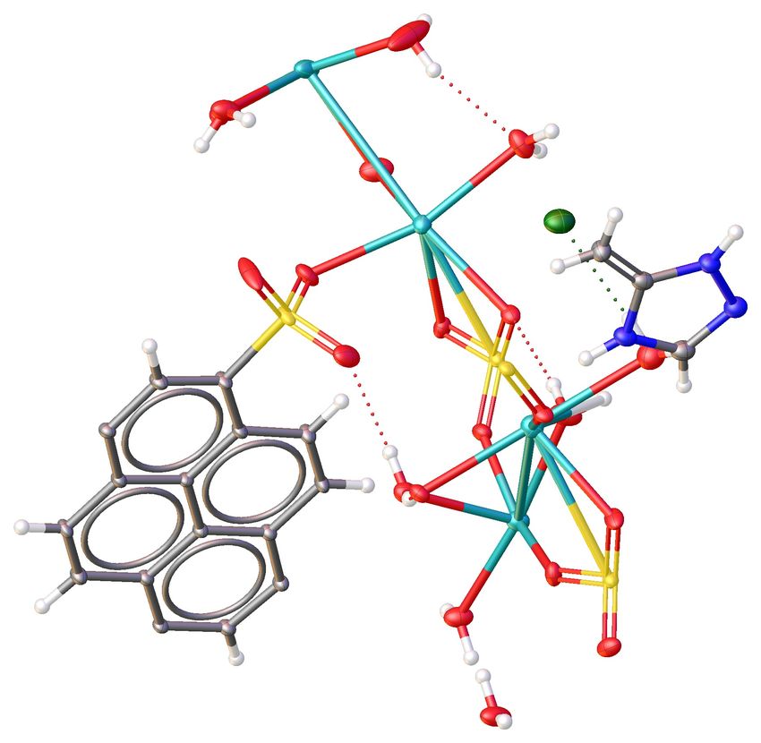
Example - ecryst377
IAM Refinement Hirshfeld Atomic Refinement
R1 = 0.0409; ∆ρmin = −0.611; R1 = 0.0343; ∆ρmin = −0.282;
∆ρmax = 0.496 ∆ρmax = 0.239
Isocontour levels from -0.6 to 0.5 eÅ−3 in steps of 0.05 eÅ−3 (red negative; blue positive)
HAR QM calculations: Hartree-Fock; spinorbital: restricted; basis set: def2-SVP
Experimental data resolution (according to Dauter - Acta Cryst. D55, 1703-1717, 1999): 0.77 Å
AvdLHirshfeld methods and Quantum Crystallography
Hirshfeld analysis
Hirshfeld atomic refinements
Benefits of Hirshfeld Atomic Refinement
I free refinement of hydrogen positions possible → hydrogens at
neutron positions
I free refinement of hydrogen isotropic or anisotropic ADP’s
possible
I but (ecryst377):
I classical refinement: Npar = 78; Nref (I > 2σ(I)) = 836
I Hirshfeld refinement: Npar = 109; Nref (I > 2σ(I)) = 836
I ADP’s of all atoms become ’neutron’ like
I modeling of density ’inside’ chemical bondsHirshfeld methods and Quantum Crystallography
Hirshfeld analysis
Hirshfeld atomic refinements
Validation of Hirshfeld Atomic Refinement results
Criteria
I do not use CheckCif !
I are R-factors lower?
I is there less residual electron density?
I are hydrogens at neutron positions?
I hydrogen ADP’s: Hirshfeld rigid body test
I the relative vibrational motion of a pair of bonded atoms has an
effectively vanishing component in the direction of the bond
2 2
I |zAB (A) − zBA (B)| < 5σ
I use platon: calc TMA 40 12 HINCL
AvdLHirshfeld methods and Quantum Crystallography
Hirshfeld analysis
Hirshfeld atomic refinements
PLATON listing file
AvdLHirshfeld methods and Quantum Crystallography
Hirshfeld analysis
Hirshfeld atomic refinements
Limitations of Hirshfeld Atomic Refinement
Limitations
I Computational cost - 3 hours and 16 processors for 20 atoms -
scales with N up to N 2.5
I Molecular wavefunctions are used, so coordination polymers or
inorganic structures not feasible
I Supramolecular features not well reproduced (polarization...)
I Hirshfeld partitioning not unique
I Disorder can not be treated, nor aperiodicity
I Only isolated molecules, no extended polymeric-like structures
AvdLHirshfeld methods and Quantum Crystallography
Hirshfeld analysis
Hirshfeld atomic refinements
Hirshfeld Atomic Refinement vs Multipole modelling
What is better ?
I Multipole modelling uses the experimental density
I Hirshfeld Atomic Refinement uses a calculated density
I Anisotropic refinement of hydrogens (nearly) not possible with
multipole modelling
I ADP’s hydrogens from HAR and neutron refinements
comparable
Will Hirshfeld Atomic Refinement replace IAM refinement and even
multipole refinement?
Fugel, ..., Puschmann et al., IUCrJ 5, 32-44 (2018)
AvdLHirshfeld methods and Quantum Crystallography
Software
Contents
From theory to practice
I Electron density and chemical bonding
I Experimental and theoretical modelling of electron densities
I Hirshfeld analysis
I Hirshfeld surfaces
I Hirshfeld refinement
I Software
I Tonto & CrystalExplorer
I Tonto & OLEX2
AvdLHirshfeld methods and Quantum Crystallography
Software
Tonto, CrystalExplorer & OLEX2
Tonto characteristics
I For quantum chemistry and quantum crystallography
I Free under the LGPL license
I Coded in Fortran, interfaced using the Foo scripting language
I Hartree-Fock and DFT calculations
I Backend for
I CrystalExplorer (GUI)
I OLEX2 - interfaces to the Hirshfeld Atomic Refinement part of
TONTO
AvdLHirshfeld methods and Quantum Crystallography
Software
Time for the demos !
AvdLYou can also read