Mapping potential signs of gas emissions in ice of Lake Neyto, Yamal, Russia, using synthetic aperture radar and multispectral remote sensing data
←
→
Page content transcription
If your browser does not render page correctly, please read the page content below
The Cryosphere, 15, 1907–1929, 2021
https://doi.org/10.5194/tc-15-1907-2021
© Author(s) 2021. This work is distributed under
the Creative Commons Attribution 4.0 License.

Mapping potential signs of gas emissions in ice of Lake Neyto,
Yamal, Russia, using synthetic aperture radar and
multispectral remote sensing data
Georg Pointner1,2,3 , Annett Bartsch1,2,3 , Yury A. Dvornikov4 , and Alexei V. Kouraev5,6
1 b.geos,
        Korneuburg, Austria
2 AustrianPolar Research Institute, Vienna, Austria
3 Department of Geoinformatics – Z_GIS, DK GIScience, Paris Lodron University of Salzburg, Salzburg, Austria
4 Department of Landscape Design and Sustainable Ecosystems, Agrarian-Technological Institute, Peoples’ Friendship

University of Russia, Moscow, Russia
5 LEGOS, Université de Toulouse, CNES, CNRS, IRD, UPS, Toulouse, France
6 Department of Geology and Geography, Tomsk State University, Tomsk, Russia

Correspondence: Georg Pointner (georg.pointner@bgeos.com)

Received: 7 August 2020 – Discussion started: 24 August 2020
Revised: 3 March 2021 – Accepted: 3 March 2021 – Published: 20 April 2021

Abstract. Regions of anomalously low backscatter in C-         supporting the hypothesis that anomalies may be related to
band synthetic aperture radar (SAR) imagery of lake ice of     gas emissions. Further, a significant expansion of backscat-
Lake Neyto in northwestern Siberia have been suggested to      ter anomaly regions in spring is documented and quantified
be caused by emissions of gas (methane from hydrocarbon        in all analysed years 2015 to 2019. Our study suggests that
reservoirs) through the lake’s sediments. However, to assess   the backscatter anomalies might be caused by lake ice sub-
this connection, only analyses of data from boreholes in the   sidence and consequent flooding through the holes over the
vicinity of Lake Neyto and visual comparisons to medium-       ice top leading to wetting and/or slushing of the snow around
resolution optical imagery have been provided due to a lack    the holes, which might also explain outcomes of polarimet-
of in situ observations of the lake ice itself. These obser-   ric analyses of auxiliary L-band Advanced Land Observing
vations are impeded due to accessibility and safety issues.    Satellite (ALOS) Phased Array type L-band Synthetic Aper-
Geospatial analyses and innovative combinations of satel-      ture Radar-2 (PALSAR-2) data. C-band SAR data are con-
lite data sources are therefore proposed to advance our un-    sidered to be valuable for the identification of lakes showing
derstanding of this phenomenon. In this study, we assess       similar phenomena across larger areas in the Arctic in future
the nature of the backscatter anomalies in Sentinel-1 C-band   studies.
SAR images in combination with very high resolution (VHR)
WorldView-2 optical imagery. We present methods to au-
tomatically map backscatter anomaly regions from the C-
band SAR data (40 m pixel spacing) and holes in lake ice       1   Introduction
from the VHR data (0.5 m pixel spacing) and examine their
spatial relationships. The reliability of the SAR method is    Lakes and ponds are common features of the Arctic con-
evaluated through comparison between different acquisition     tinuous permafrost zone and play an important role in the
modes. The results show that the majority of mapped holes      carbon cycle (e.g. Walter Anthony et al., 2012; Wik et al.,
(71 %) in the VHR data are clearly related to anomalies in     2016). Methane (CH4 ) is a powerful greenhouse gas, and the
SAR imagery acquired a few days earlier, and similarities to   global trend of its atmospheric concentration has shown sig-
SAR imagery acquired more than a month before are evident,     nificant changes over the last few decades. The concentra-
                                                               tion increased significantly until 1998 and from 2007 until

Published by Copernicus Publications on behalf of the European Geosciences Union.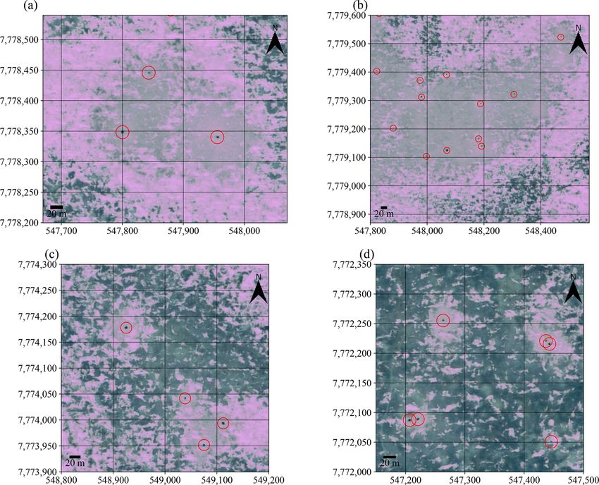
1908                                        G. Pointner et al.: Mapping potential signs of gas emissions in ice of Lake Neyto

today, while between 1999 and 2006, it remained nearly con-         lake ice associated with subcap seeps along boundaries of
stant (Nisbet et al., 2014). To date, the factors and dominant      permafrost thaw and glacial retreat in Alaska and Greenland.
sources of emissions driving these changes are not fully un-           Similar holes or zones of very thin ice in spring lake ice
derstood (e.g. Nisbet et al., 2019; Schwietzke et al., 2016).       attributed to subcap gas emissions have been described for
CH4 produced by microorganisms in the sediments of Arc-             lakes on the Yamal Peninsula in northwestern Siberia, Rus-
tic lakes can escape to the atmosphere through upward bub-          sia, by Bogoyavlensky et al. (2019a, 2016). Numerous crater-
bling (ebullition) in the water column and contributes signif-      like depressions on the bottom of a large number of lakes
icantly to the total global methane emissions (e.g. Bastviken       have also been identified and attributed to gas emissions (Bo-
et al., 2011, 2004). In addition to that, geologic methane ac-      goyavlensky et al., 2019a, b, c, 2016). However, Dvornikov
cumulated in sub-surface hydrocarbon reservoirs, previously         et al. (2019) provide alternative explanations for the origin
sealed by permafrost or glaciers that act as a cryosphere cap,      of these crater-like depressions, such as the degradation of
can also seep into the atmosphere through lake sediments and        tabular ground ice or the existence of former river valleys in
the water column in the case of open taliks under big lakes         the case of channel-like depressions and suggest that multi-
and rivers in the continuous permafrost zone or in regions of       ple origins are plausible.
glacial retreat (Walter Anthony et al., 2012).                         The Yamal Peninsula is known for its abundant gas re-
   Global climate models may currently underestimate car-           serves stored in numerous gas fields scattered all over the
bon emissions from permafrost environments significantly            peninsula (e.g. Bogoyavlensky et al., 2019b) and other phe-
and cannot account for methane ebullition from geologi-             nomena associated with the release of pressurised gas, such
cal lake seeps (Turetsky et al., 2020). Gas-emission-related        as a number of gas emission craters (GECs) that have been
phenomena can pose serious threats to humans, e.g. people           discovered and described in recent years (e.g. Bogoyavlen-
working in the gas industry or local indigenous people. The         sky et al., 2016; Dvornikov et al., 2019; Kizyakov et al.,
Yamal-Nenets are reindeer herders that travel across the Ya-        2020, 2017; Leibman et al., 2014). Many studies concerning
mal Peninsula in Western Siberia and frequently cross frozen        mapping and characterising superficial seeps in lake ice are
lakes in winter. Patches of thin ice, caused by emissions of        available for Alaskan and Swedish lakes (e.g. Lindgren et al.,
natural gas, may be present on some of these lakes (e.g.            2019, 2016; Walter et al., 2006; Wik et al., 2011). Apart from
Bogoyavlensky et al., 2016, 2019a). In June 2017, a pow-            the study by Walter Anthony et al. (2012) mentioned above,
erful explosion from a gas-inflated mound that formed un-           recent studies concerning signs of subcap seepage in lake ice
der a riverbed near Seyakha on the Yamal Peninsula, which           (Bogoyavlensky et al., 2019a, 2018, 2016) have focused on
has been documented by Bogoyavlensky et al. (2019c), scat-          lakes on the Yamal Peninsula.
tered debris over a radius of a few hundred metres. Under-             Promising in this context are space-borne synthetic aper-
standing where different forms of gas release happen may be         ture radar (SAR) data. SAR has proven to be very useful
favourable for identifying areas of increased risk for humans.      for the monitoring of lake ice phenology (e.g. Duguay and
   Walter Anthony et al. (2012) use two main terms for types        Pietroniro, 2005; Surdu et al., 2015). Several studies have
of methane seeps in lake sediments: superficial seeps and           successfully used SAR data to distinguish between ground-
subcap seeps. The former refers to seepage of ecosystem             fast (ice that has frozen to the lakebed) and floating (e.g.
methane that is continuously formed and released without            Bartsch et al., 2017; Duguay and Lafleur, 2003; Engram
storage over geological timescales. Subcap seeps are in con-        et al., 2018; Grunblatt and Atwood, 2014; Surdu et al., 2014)
trast characterised by the release of 14 C-depleted methane         lake ice. In C-band SAR images, low backscatter is observed
that has been previously sealed by the cryosphere cap. Possi-       from ground-fast lake ice and high backscatter is usually ob-
ble origins of subcap methane are microbial, thermogenic or         served from floating lake ice (Duguay and Pietroniro, 2005).
mixed microbial–thermogenic processes within sedimentary            The magnitude of the reported differences between backscat-
basins, including conventional natural gas reservoirs, coal         ter from ground-fast and floating lake ice varies across stud-
beds, buried organics associated with glacial sequences and         ies and depends on radar frequency, polarisation, incidence
potentially methane hydrates. Walter Anthony et al. (2012)          angle and geographic region (Antonova et al., 2016). Lake
identified locations of subcap and strong superficial seeps         ice is nearly transparent for the radar signal. Low radar return
during aerial and ground surveys in Alaska and Greenland            is observed from ground-fast lake ice due to low dielectric
as open holes (so-called hotspots) in winter lake ice. Among        contrast between ice and the lake sediments (Duguay et al.,
other factors, flux rates and sizes of the holes in lake ice were   2002). On the other hand, strong reflection of the radar sig-
used by the authors to distinguish superficial seeps from sub-      nal occurs at the ice–water interface of floating lake ice be-
cap seeps. Subcap methane flux rates are significantly higher       cause of high dielectric contrast between ice and liquid water
than those of superficial seeps, and the areas of open holes        (Duguay et al., 2002; Engram et al., 2013). The dielectric
were reported to be significantly larger for subcap seeps           contrast is determined by differences in the complex-valued
(up to 300 m2 ) when compared to superficial seeps (0.01–           relative permittivity ε, which in general depends on the radar
0.3 m2 ). The authors identified more than 150 000 holes in         frequency and temperature. The real part ε 0 of ice is approx-
                                                                    imately 3.17 and nearly independent of radar frequency and

The Cryosphere, 15, 1907–1929, 2021                                                    https://doi.org/10.5194/tc-15-1907-2021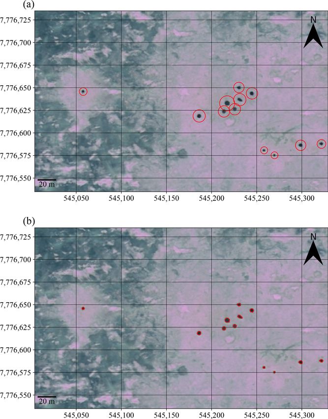
G. Pointner et al.: Mapping potential signs of gas emissions in ice of Lake Neyto                                           1909

temperature (Mätzler and Wegmüller, 1987). The imaginary           ods to map the backscatter anomalies from Sentinel-1 SAR
part ε 00 is below 10−3 for pure and impure freshwater ice at      imagery and the holes from WorldView-2 data with state-of-
C- and L-band frequencies (Mätzler and Wegmüller, 1987).           the-art image processing techniques and compare their lo-
Meissner and Wentz (2004) provide a detailed list of ε values      cations spatially. Further, we provide time series of classi-
of water at various frequencies and temperatures. At 1.7 GHz       fied area of anomalies, quantify the expansion over time and
and 25 ◦ C, ε 0 is 78 and ε 00 is 6. At 5.35 GHz and 25 ◦ C, ε 0   discuss the use of other remote sensing data that could help
is 73 and ε 00 is 19. At 5 GHz and −4 ◦ C, ε 0 is 65 and ε 00      to advance the understanding of the mechanisms involved.
is 38. ε of frozen soil largely depends on the temperature         In this regard, investigations of Advanced Land Observing
and on the water, clay, silt and sand content (Zhang et al.,       Satellite (ALOS) Phased Array type L-band Synthetic Aper-
2003). At 10 GHz, ε 0 ranges approximately from 3.2 to 8 and       ture Radar-2 (PALSAR-2) fully polarised L-band SAR data
ε 00 from 0.1 to 2 (Hoekstra and Delaney, 1974). Little sen-       were carried out, which could reveal the dominant scattering
sitivity of ε of frozen soil to the radar frequency between        mechanisms of backscatter from anomaly regions and regu-
1.4 and 10.6 GHz is suggested by estimates in Zhang et al.         lar floating lake ice.
(2003). The reported values were chosen since they were
most representative of the SAR data (C- and L-band) used
in this study. The dominant mechanism for high backscat-           2   Study site
ter from floating lake ice observed by SAR sensors has long
been described to be double-bounce scattering from the ice–        Lake Neyto (other title – Neyto-Malto), 70.073◦ N,
water interface and columnar bubbles trapped within the ice        70.350◦ E, is located in the central part of the Yamal Penin-
(e.g. Duguay et al., 2002; Jeffries et al., 1994; Wakabayashi      sula, ca. 80 km away from the closest settlement of Seyakha
et al., 1993). More recent studies, however, provide strong        and about 80 km away from the Bovanenkovo gas field. The
evidence that the dominant mechanism is direct backscatter-        lake has the second-largest area (214 km2 ) in Yamal after
ing from a rough ice–water interface (Atwood et al., 2015;         Lake Yarroto-1. The length of the shoreline is about 60 km,
Engram et al., 2020, 2013; Gunn et al., 2018). Engram et al.       and the lake measures approximately 17.8 km in the south–
(2020) showed a significant correlation between whole-lake         north direction and 16.5 km from west to east. The lake is rel-
methane emissions and whole-lake L-band backscatter from           atively shallow, reaching 17 m at the northwest corner, but the
ice-covered Alaskan lakes in the case of superficial seeps (see    average depth does not exceed 3 m, which results in a signifi-
Sect. 6 for details).                                              cant mixing of water masses during summer (Edelstein et al.,
    For Lake Neyto on the Yamal Peninsula, regions charac-         2017). Wide shelf areas of up to 800 m can be found within
terised by low C-band backscatter that very likely belong to       the lake, whereas at the deepest part, several depressions with
the floating ice regime have been identified (Bogoyavlensky        diameters up to 500–800 m are documented (Edelstein et al.,
et al., 2018; Pointner et al., 2019). Based on the analysis of     2017). Lake shores are mostly cliffs up to 25 m high, some-
data of boreholes in the vicinity of Lake Neyto, Bogoyavlen-       times with tabular ground ice exposures. The ground temper-
sky et al. (2018) described a gas field that stretches out un-     ature at 2 m depth in the surroundings of the lake is approxi-
der Lake Neyto. They showed Sentinel-1 scenes acquired in          mately −1.5 ◦ C (Obu et al., 2020). Snow depth (liquid water
different years, compared them visually to optical Sentinel-2      equivalent) from ERA5 reanalysis data generally increases
scenes, and suggested that backscatter anomalies are related       gradually in winter and spring until melt onset and has typi-
to zones of very thin or no ice which resulted from gas bub-       cally ranged between 15 and 20 cm at its maximum in recent
ble inclusions within the ice. Pointner et al. (2019) also sug-    years (Hersbach et al., 2018).
gested that the regions of low backscatter may be a result of         Figure 1 shows the location of Lake Neyto in the
up-welling gas released through the sediments, which might         Arctic and a comparison between Sentinel-1 Extra Wide
lead to local thinning of the ice or that eddies might cause a     (EW) swath horizontal–horizontal (HH)-polarised imagery,
local thinning of the ice layer, which is similar to the cause     a Sentinel-2 true-colour composite and a subset of a
of ice rings on lakes Baikal, Hövsgöl and Teletskoye reported      WorldView-2 true-colour composite for Lake Neyto in
by Kouraev et al. (2019, 2016).                                    May 2016, where all images were acquired within 6 d. The
    In this study, we demonstrate a connection between po-         mentioned anomalies of low backscatter surrounded by re-
tential signs of gas emissions in SAR and optical very high        gions of much higher backscatter in regions of assumed float-
resolution (VHR) imagery of Lake Neyto for the first time.         ing lake ice (based on the bathymetric map of Lake Neyto by
We provide a direct link between the locations of clusters         Edelstein et al., 2017, and expectable maximum ice thick-
of low backscatter from Sentinel-1 SAR data and poten-             ness of 1.5 to 2 m for lakes in Yamal; Bogoyavlensky et al.,
tial seep sites that we could identify as open holes in lake       2018) can be seen in Fig. 1b. Figure 1c shows a Sentinel-2
ice in a single VHR WorldView-2 image. Similar holes in            image acquired 5 d later. Strong similarities to the Sentinel-1
VHR imagery were described and shown in detail for Lake            image can be identified easily. Locations of clusters of low
Otkrytie, located approximately 60 km to the east of Lake          backscatter in the SAR imagery apparently resemble regions
Neyto, by Bogoyavlensky et al. (2019a). We present meth-           where the snow has melted earlier than in other regions in

https://doi.org/10.5194/tc-15-1907-2021                                                 The Cryosphere, 15, 1907–1929, 2021
1910                                      G. Pointner et al.: Mapping potential signs of gas emissions in ice of Lake Neyto

Table 1. Years of Sentinel-1 EW data and associated numbers of       We used IW data for validation purposes and visual com-
images and average temporal gaps.                                 parisons. A validation was carried out that compared classi-
                                                                  fied anomalies from EW images and IW images that were
              Year    Number of        Average                    acquired on consecutive dates (for details see Sect. 4.3). The
                        images     temporal gap                   local acquisition dates and times (LT) of these validation data
              2015            29         4d 7h                    are shown in Table 2.
              2016            88        1 d 13 h                     Lists of the used scenes including the mean projected
              2017           112         1d 7h                    local incidence angle over the lake, acquisition times
              2018            52        2 d 23 h                  in local time and coordinated universal time (UTC),
              2019            41        3 d 14 h                  and an indicator showing if the scenes were assembled
                                                                  due to slicing (see Sect. 4.1.1) are provided in the Sup-
                                                                  plement (Tables S1–S4) to this article in CSV format.
the optical image. Figure 1d shows a detail (marked by the        “S1__scene_metadata_list_Sentinel1_EW_main.csv”
red rectangle in Fig. 1b and c) of a WorldView-2 acquisition      contains a list of the main Sentinel-1 EW data (342
taken 1 d after the Sentinel-2 acquisition. Dark spots on white   scenes) used in this study. “S2__scene_metadata_list_ Sen-
regions are visible that we interpret as open holes surrounded    tinel1_EW_lake_masks.csv” and “S3__scene_metadata_
by regions of bright ice, slush or snow. A similarity to open     list_Sentinel1_EW_shelf_masks.csv” contain lists of
holes in ice associated with gas emissions described by Bo-       the Sentinel-1 EW data used for calculating lake
goyavlensky et al. (2019a) and Walter Anthony et al. (2012)       masks (5 scenes) and shelf masks (5 scenes), re-
is apparent, and such holes can be found over wider regions       spectively (see Sect. 4.2.1 for details). “S4__scene_
of Lake Neyto in the WorldView-2 image.                           metadata_list_Sentinel1_IW.csv” contains a list of all
                                                                  Sentinel-1 IW data used for the validation (10 scenes).
                                                                  “S5__scene_metadata_list_other_sensors.csv” contains a
3     Data                                                        similar list for the other satellite data (4 scenes in total)
                                                                  used in this study, which are described in the following
3.1    Sentinel-1 synthetic aperture radar data                   paragraphs.
The two polar-orbiting satellites Sentinel-1A and Sentinel-
                                                                  3.2   WorldView-2 very high resolution optical data
1B are part of the European Union’s (EU) Copernicus pro-
gramme. They were launched into orbit in April 2014 and
                                                                  The WorldView-2 satellite was launched in October 2009 and
in April 2016. The identical SAR sensor on both satellites,
                                                                  is operated by Maxar Technologies (formerly DigitalGlobe).
called C-SAR, can be operated in different acquisition and
                                                                  It was the first commercial satellite to collect data at a very
polarisation modes at a centre frequency of 5.405 GHz. The
                                                                  high spatial resolution in eight spectral bands. WorldView-2
acquisition modes differ from each other in terms of spatial
                                                                  data include a panchromatic band covering the wavelength
resolution and swath width. Data can be acquired in either
                                                                  range from 450 to 800 nm. The spatial resolution is 1.84 m
single co-polarised or dual co-polarised plus cross-polarised
                                                                  for the multispectral bands and 0.46 m for the panchromatic
channels (European Space Agency, 2012).
                                                                  band (Padwick et al., 2010). For this study, 100 km2 of or-
   The default operating mode over land is the Interferomet-
                                                                  thorectified WorldView-2 imagery (eight multispectral bands
ric Wide (IW) swath mode with vertical–vertical (VV) and
                                                                  plus one panchromatic band) from 22 May 2016 covering ap-
vertical–horizontal (VH) dual-polarised acquisitions (Eu-
                                                                  proximately half of the surface area of Lake Neyto was avail-
ropean Space Agency, 2012). However, acquisitions over
                                                                  able.
Lake Neyto are most frequently taken in Extra Wide (EW)
swath mode with horizontal–horizontal (HH) and horizontal–
                                                                  3.3   ALOS PALSAR-2 fully polarised SAR data
vertical (HV) dual polarisation. EW data are acquired at
larger swath widths compared to IW data, but IW data have
                                                                  The PALSAR-2 sensor on board the Advanced Land Ob-
a finer spatial resolution than EW data. Commonly used
                                                                  serving Satellite-2 (ALOS-2) is the successor to the PAL-
pixel spacing after the pre-processing steps is 40 m in EW
                                                                  SAR instrument on ALOS and operates at slightly vary-
mode and 10 m in IW mode. The number of EW acquisitions
                                                                  ing centre frequencies of between 1.237 and 1.279 GHz
over Lake Neyto is significantly larger (Pointner and Bartsch,
                                                                  (Kankaku et al., 2013). ALOS-2 was launched in May 2014
2020), and no acquisitions in IW mode were taken in 2016.
                                                                  and is operated by the Japan Aerospace Exploration Agency
Hence, the primary SAR data for our analyses were Sentinel-
                                                                  (JAXA). Similarly to Sentinel-1, PALSAR-2 can be op-
1 EW data with both HH and HV polarisation channels. Ta-
                                                                  erated in different imaging modes with varying ground
ble 1 shows the years of data, the number of Sentinel-1 EW
                                                                  resolutions and swath widths, but it is able to acquire
images and the average temporal gap between the image ac-
                                                                  data in single-polarisation (HH, HV, VH or VV), dual-
quisitions in the years concerned.
                                                                  polarisation (HH + HV or VV + VH) and full-polarisation

The Cryosphere, 15, 1907–1929, 2021                                                  https://doi.org/10.5194/tc-15-1907-2021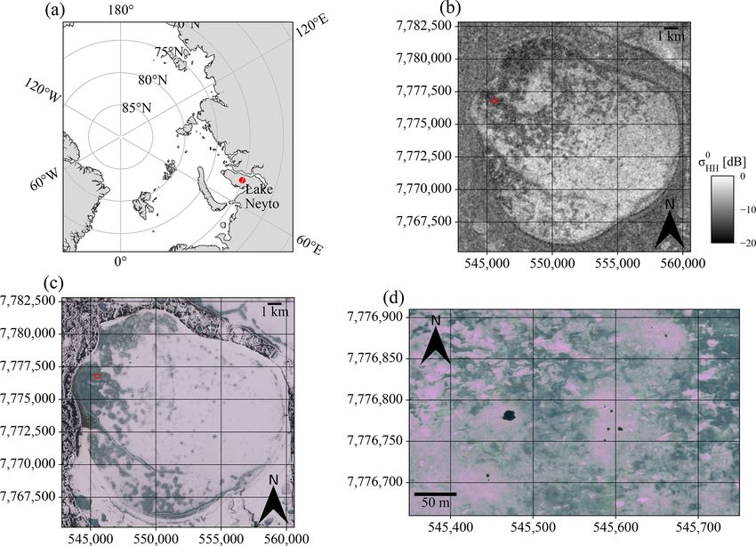
G. Pointner et al.: Mapping potential signs of gas emissions in ice of Lake Neyto                                                   1911

Figure 1. Location of Lake Neyto and visual comparison of potential signs of gas emissions in satellite data. (a) Location of Lake Neyto
in the Arctic. (b) Backscatter anomalies are visible as clusters of low backscatter surrounded by regions of much higher backscatter in a
Sentinel-1 EW HH-polarised acquisition from 16 May 2016. (c) Regions where snow seems to have melted earlier that appear similar to the
regions of backscatter anomalies in the Sentinel-1 image can be seen in a Sentinel-2 true-colour composite from 21 May 2016. (d) Zoomed-in
view of a WorldView-2 true-colour composite from 22 May 2016, where holes in the ice are visible as dark spots surrounded by very bright
ice. The red rectangle in (b) and (c) indicates the region of the zoomed-in view in (d). Coordinate reference system (CRS): (a) WGS 84 /
Arctic Polar Stereographic, (b)–(d) WGS 84 / UTM zone 42N.

Table 2. Local acquisition dates and times of pairs of Sentinel-1 EW and IW scenes used for validation.

                              S1 EW local acquisition date and time    S1 IW local acquisition date and time
                              22 May 2017, 07:02:36 LT                 23 May 2017, 06:53:47 LT
                              29 January 2018, 07:02:39 LT             30 January 2018, 06:53:51 LT
                              10 February 2018, 07:02:39 LT            11 February 2018, 06:53:51 LT
                              24 February 2018, 06:46:13 LT            23 February 2018, 06:53:51 LT
                              6 March 2018, 07:02:39 LT                7 March 2018, 06:53:51 LT
                              30 March 2018, 07:02:40 LT               31 March 2018, 06:53:51 LT
                              23 April 2018, 07:02:40 LT               24 April 2018, 06:53:52 LT
                              19 May 2018, 06:46:16 LT                 18 May 2018, 06:53:53 LT
                              31 May 2018, 06:46:16 LT                 30 May 2018, 06:53:54 LT
                              24 May 2019, 07:02:48 LT                 25 May 2019, 06:54:00 LT

(HH + HV + VH + VV) modes (Kankaku et al., 2013). In                    3.4   Sentinel-2 medium resolution optical data
this study, we used an ALOS PALSAR-2 fully (quad-
)polarised scene in High-Sensitive Stripmap mode from
18 April 2015, which was acquired at a swath width of 50 km             Sentinel-2A and Sentinel-2B are also part of the EU’s Coper-
and a ground resolution of approximately 6 m (Kankaku                   nicus programme and were launched into orbit in June 2015
et al., 2013) for polarimetric analyses to infer possible scat-         and March 2017, respectively. The two satellites carry an
tering mechanisms for anomaly regions and regular floating              identical multispectral instrument which acquires data in 12
lake ice.                                                               spectral bands in the optical, near-infrared and short-wave
                                                                        infrared range (Drusch et al., 2012). The spatial resolution
                                                                        varies between bands and is 10, 20 or 60 m. The red, green
                                                                        and blue bands have a spatial resolution of 10 m. In this study,

https://doi.org/10.5194/tc-15-1907-2021                                                        The Cryosphere, 15, 1907–1929, 2021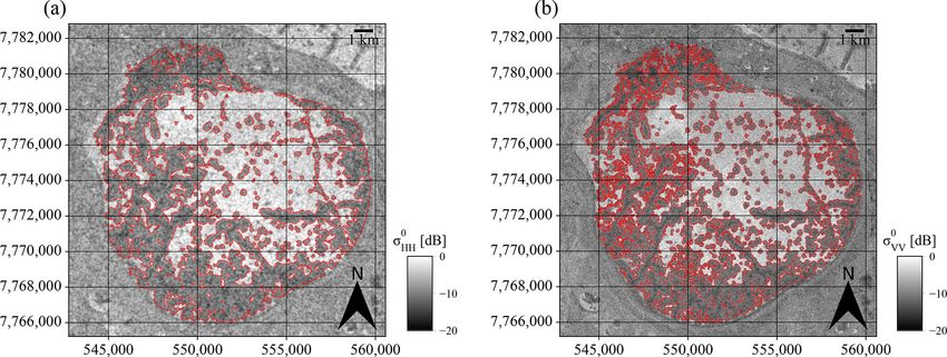
1912                                        G. Pointner et al.: Mapping potential signs of gas emissions in ice of Lake Neyto

Sentinel-2 true-colour composites based on the 10 m resolu-         Table 3. Polynomial coefficients used for the incidence angle nor-
tion bands were used for visual interpretations.                    malisation with respect to the sensor mode and polarisation.

3.5     Landsat 8 brightness temperature and surface                                            a            b           c
        reflectance
                                                                               EW HH       0.0067    −0.6784       1.7417
                                                                               EW HV       0.0026    −0.3976     −16.2692
Landsat 8 is the latest satellite of the Landsat satellite series              IW VV       0.0123    −1.1955      12.2970
that have been continuously providing multispectral data of                    IW VH       0.0148    −1.4496      10.1781
the earth’s land surface since 1972. Landsat 8 was launched
in February 2013 and carries the Operational Land Imager
(OLI) and the Thermal Infrared Sensor (TIRS) instruments.
OLI acquires data in eight spectral bands in the optical, near-     toolbox (Zuhlke et al., 2015). Some products have been
infrared and short-wave infrared range at a 30 m spatial res-       sliced directly over the lake. In these cases, the slice-
olution and in one panchromatic band at a 15 m spatial reso-        assembly operator was applied to those products in the
lution (Roy et al., 2014). TIRS collects data in two spectral       gpt as the first processing step. Products to which this
bands in the thermal infrared range at a 100 m spatial resolu-      operator was applied are indicated in Tables S1–S4. In
tion (Roy et al., 2014). We used a true-colour composite of         the following, the applied operators within the gpt were
surface reflectance and the band-10 brightness temperature          subsetting, radiometric calibration, thermal noise removal
of a Landsat 8 scene of Lake Neyto acquired on 6 April 2015         and terrain correction using the ArcticDEM version 3.0
for visual comparisons to the SAR data.                             (Porter et al., 2018). The well-known-text (WKT) rep-
                                                                    resentation of the subset extent in World Geodetic Sys-
3.6     ERA5 2 m air temperature                                    tem 84 (WGS 84) geographical coordinates is POLYGON
                                                                    ((69.2277 69.7650, 70.9744 69.7650, 70.9744 70.3610,
ERA5 is the fifth generation of European Centre for                 69.2277 70.3610, 69.2277 69.7650, 69.2277 69.7650)). Af-
Medium-Range Weather Forecasts (ECMWF) global cli-                  ter these steps, the data were converted to decibels (dB) and
mate and weather reanalysis. Reanalysis uses combined               incidence angle normalisation was performed. The incidence
model data and observations on a global scale to de-                angle normalisation methodology used here is described in
rive a complete and consistent dataset (Hersbach et al.,            Pointner et al. (2019) and uses empirically derived normal-
2018). The ERA5 product of hourly data on single levels             isation functions in the form of second-degree polynomials
from 1979 to the present contains hourly estimates for              to normalise backscatter in decibels to a common reference
a variety of atmospheric, ocean-wave and land-surface               incidence angle of 30◦ . The normalisation function can be
parameters on a regular latitude–longitude grid of 0.25◦            written as
(Hersbach et al., 2018). In this study, we used the “2 m
temperature” variable, which represents near-surface air             0
                                                                    σnorm (θ ) [dB] = a · θ 2 + b · θ + c,                        (1)
temperature, for a comparison to the temporal dynamics
of the backscatter anomalies. The 2 m temperature data
                                                                              0
for the nearest grid point to Lake Neyto (70◦ N, 70.25◦ E)          where σnorm   (θ ) is the normalisation function; θ is the local
were therefore aggregated to daily minima and max-                  projected incidence angle; and a, b and c are the polynomial
ima using the cdstoolbox.geo.extract_point                          coefficients. The polynomial coefficients in Eq. (1) used for
and      cdstoolbox.climate.daily_min                 and           the incidence angle normalisation with respect to the sensor
cdstoolbox.climate.daily_max                methods     of          mode and polarisation are given in Table 3.
the Python application programming interface (API) of the              Based on these coefficients, the final normalisation to the
Copernicus Climate Change Service (C3S) Climate Data                reference incidence angle of 30◦ was applied using (Pointner
Store (CDS). The data were subsequently downloaded and              et al., 2019)
converted to degrees Celsius.
                                                                    σ 0 (30) = σ 0 (θ ) − (σnorm
                                                                                            0            0
                                                                                                 (θ ) − σnorm (30)),              (2)

4     Methods
                                                                    where σ 0 (30) is the backscatter coefficient normalised to
4.1     Pre-processing of satellite data                            30◦ , σ 0 (θ ) is the backscatter coefficient before normalisa-
                                                                            0
                                                                    tion, σnorm   (θ ) is the value of the normalisation function at
                                                                    the incidence angle concerned and σnorm  0  (30) is the value of
4.1.1    Pre-processing of Sentinel-1 SAR data
                                                                    the normalisation function at 30 .  ◦

The majority of pre-processing steps for Sentinel-1 EW                 All steps were applied to both polarisation channels (HH
and IW data were conducted with the graph processing                and HV for EW mode, VV and VH for IW mode). Outputs
tool (gpt) of the Sentinel Application Platform (SNAP)              were images of normalised backscatter coefficient σ 0 .

The Cryosphere, 15, 1907–1929, 2021                                                      https://doi.org/10.5194/tc-15-1907-2021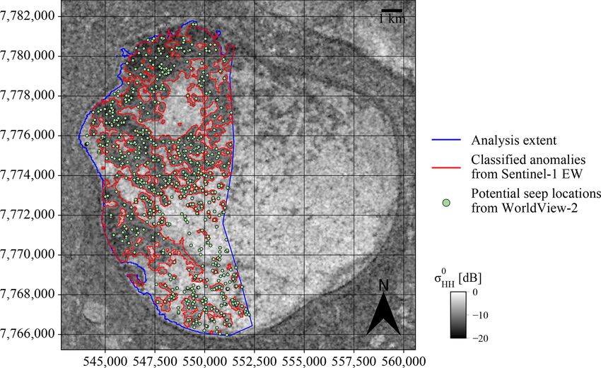
G. Pointner et al.: Mapping potential signs of gas emissions in ice of Lake Neyto                                             1913

4.1.2   Pre-processing of optical imagery                           4.2     Classification and detection methods

We calibrated the WorldView-2 data from 22 May 2016 to              4.2.1    Classification of backscatter anomalies from
top-of-atmosphere (TOA) reflectance following the method-                    Sentinel-1 data
ology given by Updike and Comp (2010) and applied pan-
sharpening from the Geospatial Data Abstraction Library             The method to classify backscatter anomalies (clusters of
(GDAL) command line utilities (version 2.2.4) which is              unusually low backscatter) in Sentinel-1 SAR images was
based on the Brovey method (GDAL/OGR contributors,                  briefly outlined in Pointner and Bartsch (2020) but is given
2020) using all available bands.                                    here in greater detail. The input for the classification algo-
  Sentinel-2 data were downloaded in level-1C (L1C) for-            rithm is pre-processed Sentinel-1 images of σ 0 in decibels
mat and directly used for visual comparisons.                       after incidence angle normalisation. All steps described in
                                                                    the following were identically performed on both polarisa-
4.1.3   Polarimetric processing of ALOS PALSAR-2                    tion channels. The most important software packages used
        fully polarised SAR data                                    for the classification were the Python packages scikit-image
                                                                    (skimage) version 0.15.0 (van der Walt et al., 2014), GDAL
From the fully polarised ALOS PALSAR-2 data in High-
                                                                    version 2.2.4 (GDAL/OGR contributors, 2020), SciPy ver-
Sensitive Stripmap mode acquired on 18 April 2015, we de-
                                                                    sion 1.1.0 (Virtanen et al., 2020) and NumPy version 1.15.1
duced two polarimetric products in order to infer scattering
                                                                    (Harris et al., 2020).
properties of regular floating lake ice and anomaly regions.
                                                                       As a first step, areas outside the lake and the shelf
Firstly, we calculated the coherency matrix T3 (Lee and Pot-
                                                                    area of the lake, where ground-fast ice is assumed,
tier, 2009), of which the first element T11 has been shown
                                                                    were masked. We deduced lake masks from late-autumn
to relate to surface scattering and correlate with the area of
                                                                    Sentinel-1 EW imagery and shelf masks from winter
gas bubbles trapped in lake ice and methane flux estimates
                                                                    Sentinel-1 EW imagery through binary classification for
of ice-covered lakes in Alaska (Engram et al., 2020, 2013).
                                                                    each year separately. For the extraction of the lake masks,
The calculations were performed in SNAP, and the process-
                                                                    we used Otsu thresholding (Otsu, 1979) on the HH-
ing steps were radiometric calibration, calculation of T3 (Lee
                                                                    polarisation band (σ 0 in dB) implemented in scikit-image
and Pottier, 2009), polarimetric speckle filtering using the re-
                                                                    (skimage.filters.threshold_otsu, default pa-
fined Lee filter (Lee et al., 2008), terrain correction using the
                                                                    rameters) of the late-autumn acquisitions. Here, no incidence
ArcticDEM and spatial subsetting. Secondly, we performed
                                                                    angle normalisation was applied, as the incidence angle
an unsupervised polarimetric classification using the method
                                                                    range over the lake was small and the backscatter values were
proposed by Cloude and Pottier (1997), which can allow for
                                                                    only used to create the masks and were not compared to those
a detailed identification of scattering mechanisms. In com-
                                                                    of other acquisitions. After thresholding, we used the method
parison with the calculation of T3 , the workflow was essen-
                                                                    scipy.ndimage.morphology.binary_fill_
tially the same, with the only difference being that between
                                                                    holes (default parameters) to fill holes in the classification
the polarimetric speckle filtering and terrain correction steps,
                                                                    result, polygonised the result using gdal_polygonize.py
the polarimetric classification was computed. The classifica-
                                                                    (default parameters) and extracted the polygon of Lake
tion itself consists of two main steps. The first step is the po-
                                                                    Neyto. Images used for the classification were cropped to the
larimetric decomposition and extraction of entropy (H ) and
                                                                    extent of the lake masks. For the shelf masks, we selected
alpha (α) parameters (Cloude and Pottier, 1997; Lee and Pot-
                                                                    the latest date where clusters of low-backscatter pixels on
tier, 2009), and the second step is the classification based on
                                                                    assumed floating ice were not spatially connected to the shelf
nine discrete regions in the H -α plane (Cloude and Pottier,
                                                                    zone, where ground-fast lake ice was assumed. The shelf
1997). Each of these regions indicates the dominant scat-
                                                                    masks were computed through a binary classification on
tering mechanism in the resolution cell concerned (Cloude
                                                                    the HH-polarisation band using incidence-angle-dependent
and Pottier, 1997). The output pixel values from SNAP did
                                                                    thresholding as described by Pointner et al. (2019) and
not correspond to the zone designations in Cloude and Pot-
                                                                    extraction of all areas that were classified as ground-fast lake
tier (1997) and Lee and Pottier (2009); i.e. regions in the
                                                                    ice and connected to the lake outline. Additionally, binary
H -α plane were labelled by different numbers comparing
                                                                    dilation (skimage.morphology.dilation with
between the SNAP documentation and Cloude and Pottier
                                                                    selem=skimage.morphology.disk(3), otherwise
(1997) and Lee and Pottier (2009). Thus, we reclassified
                                                                    default parameters) was applied to this shelf mask to exclude
the output to match the designations of Cloude and Pottier
                                                                    areas that may be affected by late grounding of the lake ice
(1997) and Lee and Pottier (2009).
                                                                    in late winter or spring from the classification.
                                                                       After masking, pixel values were re-scaled
                                                                    from decibels to the interval from −1 to 1 us-
                                                                    ing       skimage.exposure.rescale_intensity
                                                                    (out_range=(-1,1); in_range=(-40,0) in the

https://doi.org/10.5194/tc-15-1907-2021                                                   The Cryosphere, 15, 1907–1929, 2021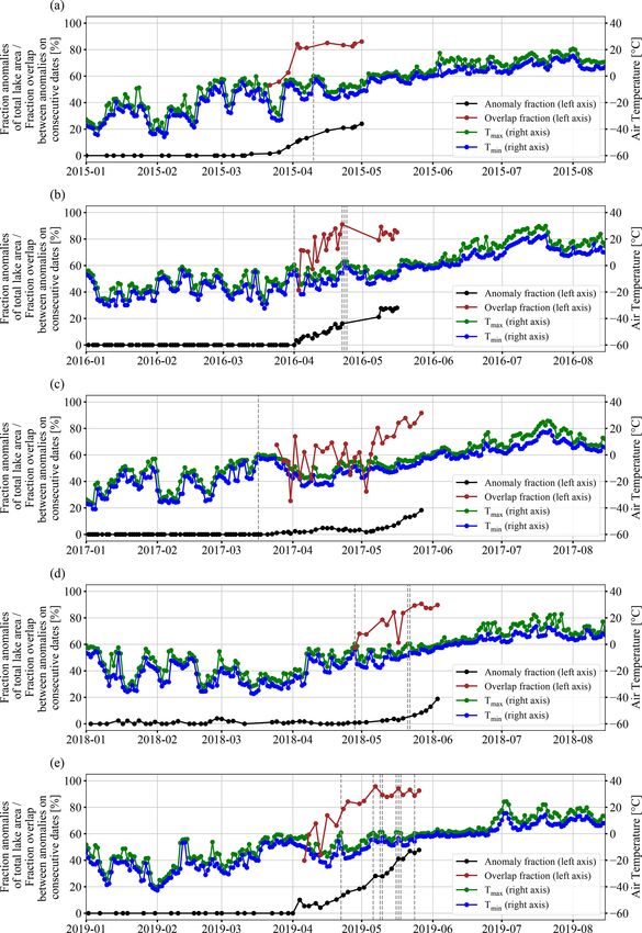
1914                                      G. Pointner et al.: Mapping potential signs of gas emissions in ice of Lake Neyto

case of co-polarisation; in_range=(-50,-10) in                    9 Sentinel-1 EW pixels from the final classification result
the case of cross polarisation), as required by the image         (skimage.morphology.remove_small_objects).
processing algorithms applied in the following. The main             Since Yen thresholding determines the threshold for the
image processing steps were bilateral filtering to reduce         binary classification automatically, it is not applicable if
noise in the images, local auto-levelling to balance out          backscatter anomalies are not present in the image. Since
the unevenly distributed backscatter level across the lake,       the mapping of clusters should be automatic, we needed to
and Yen thresholding (Yen et al., 1995) to automatically          include a test of whether anomalies were apparent in the im-
classify the images into the two categories for floating lake     ages. Our approach again utilises the dual-polarisation capa-
ice “low-backscatter anomalies” (positive class) and “high        bility of Sentinel-1 and tests the similarity between classifi-
backscatter from regular floating lake ice” (negative class).     cation outcomes of the two polarisation channels using Co-
   For      the      bilateral     filtering,    we       used    hen’s kappa score κ (Cohen, 1960). Only if κ was above 0.2
skimage.filters.rank.mean_bilateral                               (class “fair agreement” according to Landis and Koch, 1977),
(selem=skimage.morphology.square(5);                              was the final classification produced as described above. If κ
s0=20 in the case of EW; s0=150 in the                            was below 0.2, all pixels in the image were assigned to the
case of IW; s1=150 in both cases). For the                        negative class.
local    auto-levelling,     we     defined    specific    ker-      The classification method was especially designed to map
nels as NumPy arrays. In the case of EW data,                     anomalies in late-winter and spring images. A considerable
numpy.ones([51,int(image.shape[1]/4)])                            ice thickness is required to resist wind forces without break-
was      used.     In      the    case      of    IW      data,   ing on large lakes, and SAR imagery of lake ice acquired
numpy.ones([204,int(image.shape[1]/4)])                           during early periods of ice formation can exhibit features of
was used. Here, the shape of the image (image.shape)              fracturing, movement or refreezing (Duguay and Pietroniro,
had been defined by the cropping of the pre-processed             2005). Our algorithm may classify such features in autumn
images by the lake masks. These kernels were then rotated         or early-winter images incorrectly as the targeted anomalies.
using     scipy.ndimage.interpolation.rotate                      To prevent this, we restricted time series analyses to imagery
(angle=45, otherwise default parameters) by 45◦ , as              acquired after 1 January in all years concerned.
the largest backscatter gradient seemed to often occur
from northwest to southeast of the lake in many images.           4.2.2   Detection and mapping of holes in lake ice from
The local auto-levelling itself was then performed using                  WorldView-2 data
skimage.filters.rank.autolevel_percentile
(with the defined kernel and p0=0 and p1=1). Although             For the automated detection of open holes in the ice from
using 0 and 1 as percentiles, we encountered differ-              the WorldView-2 acquisition, we used a blob detector from
ent behaviour of this method regarding the treatment              scikit-image which uses the Laplacian of Gaussian (LoG)
of the no-data mask when compared to the method                   filter (van der Walt et al., 2014). The term blob stands for
skimage.filters.rank.autolevel, and thus                          “binary large object”, and the holes in the ice are considered
skimage.filters.rank.autolevel_percentile                         blobs here. The intention behind using this approach was
was      preferred.      Yen      thresholding     was       in   to automatically map dark round spots in the imagery
the following applied to the imagery using                        characterised by high contrast to the surrounding regions in
skimage.filters.threshold_yen with default                        a reproducible manner. The blob detector is a method to be
parameters.                                                       applied to greyscale imagery. We used the green band as
   The output of these steps were two classified binary im-       the input as it allowed for the best separation between holes
ages: one for the co-polarised channel (HH in EW mode, VV         and surface features that we did not interpret as holes but
in IW mode) and one for the cross-polarised channel (HV in        could have been confused with holes by the blob-detection
EW mode, VH in IW mode). The bilateral mean filter was            algorithm. The detector works by successively convolving
chosen to handle noise with the aim of binary classification      the image with LoG kernels of increasing standard deviation
in mind, as opposed to a conventional speckle filter.             and stacking up the responses in a cuboid. Detected blobs
   We      applied       a     logical      AND        operator   are local maxima in the cuboid that are filtered using an
(numpy.logical_and, default parameters) to these                  intensity threshold on the maxima. Again, we tried to be
two images to keep only pixels that belong to the class           very cautious when selecting this threshold to only detect
of backscatter anomalies in the outcome of both polar-            dark round spots characterised by significant contrast to the
isation channels. Since we had no in situ data available          surrounding pixels that are most likely holes in the lake
(see Sect. 4.3), we tried to use conservative settings            ice. The method skimage.feature.blob_log
wherever possible. In order to mitigate potential re-             (min_sigma=0.69,                           max_sigma=10,
maining noise even further, we removed connected                  num_sigma=200, threshold=0.187) was used
components (4-neighbourhood) smaller than the size of             on the negative of the green-band pan-sharpened TOA
                                                                  reflectance image. Figure 2 gives an example of what we

The Cryosphere, 15, 1907–1929, 2021                                                  https://doi.org/10.5194/tc-15-1907-2021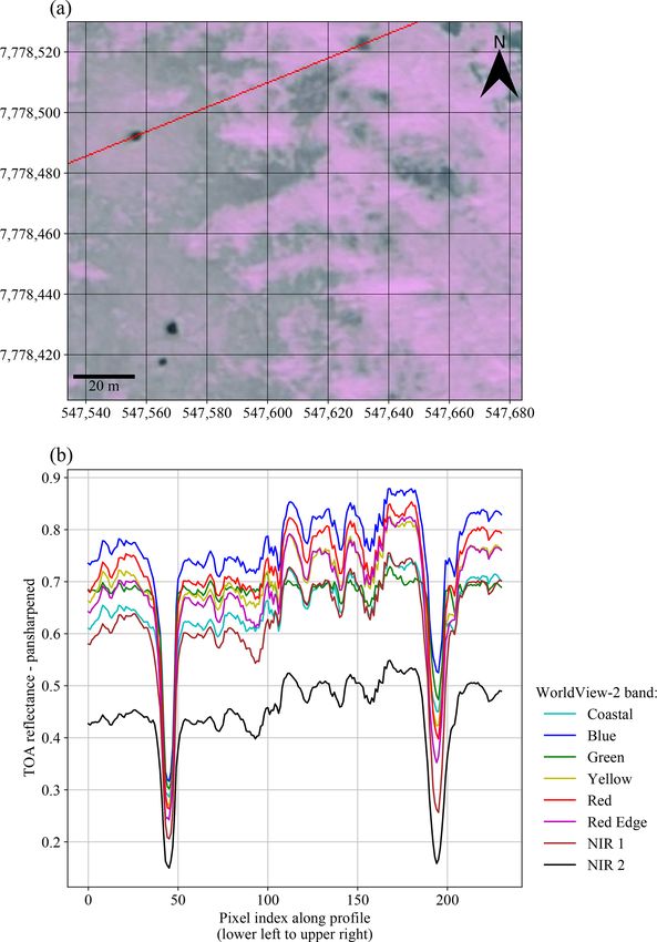
G. Pointner et al.: Mapping potential signs of gas emissions in ice of Lake Neyto                                                1915

                                                                       blob concerned. In order to estimate hole areas, we per-
                                                                       formed a binary classification based on a marker-based wa-
                                                                       tershed segmentation using the blob-detection results to clas-
                                                                       sify all pixels belonging to the holes. Markers for the hole
                                                                       class were set on single pixels on which the centres of
                                                                       detected blobs were located. Markers for the background
                                                                       class were set on pixels with pan-sharpened TOA reflectance
                                                                       larger than 0.45. The marker image was defined with the
                                                                       same size as the original image, with value 1 for the hole
                                                                       markers, value 2 for the background class and value 0 else-
                                                                       where. After the definition of the markers, the watershed
                                                                       segmentation (skimage.segmentation.watershed,
                                                                       default parameters) was applied using the original image and
                                                                       the marker image, and individual hole objects were extracted
                                                                       and vectorised. In rare cases, the watershed segmentation
                                                                       produced unsatisfactory results by clearly overflowing the
                                                                       area of the expected hole. To handle these false classifica-
                                                                       tions, we excluded all hole polygons larger than 300 m2 from
                                                                       further analysis (the largest open holes formed by subcap
                                                                       seepage in Walter Anthony et al., 2012, were reported to be
                                                                       approximately 300 m2 in area).

                                                                       4.3   Validation of Sentinel-1 classification methodology

                                                                       No in situ data were available for Lake Neyto to validate
                                                                       the classification of anomaly regions from Sentinel-1 data
                                                                       directly. The remoteness of the area and the absence of trans-
                                                                       portation infrastructure largely impedes in situ data collec-
                                                                       tion. More strikingly, it is likely that parts of the regions
                                                                       of backscatter anomalies on the lake are characterised by
Figure 2. Examples of features in WorldView-2 imagery acquired         very thin ice, which would pose a direct threat to human
on 22 May 2016 and associated spectral profile. (a) WorldView-2        safety if in situ data collection on the lake ice was attempted.
true-colour composite with red line indicating the pixels used for     Ice only a few centimetres thick was also reported by the
plotting the profile (CRS: WGS 84 / UTM zone 42N). (b) Spectral
                                                                       Yamal-Nenets on Lake Yambuto in mid-march 2017, where
profile indicating variations between contrast for the two main min-
                                                                       ice thickness at that time is usually more than 1 m (Pointner
ima. The left main minimum was considered a hole that should be
detected, while the right minimum was not considered a hole, and       et al., 2019).
its detection should be avoided.                                          Due to the lack of reference data collected at site, we pro-
                                                                       pose a comparison of classification results from EW data
                                                                       (HH and HV polarisation) and IW (VV and VH polarisa-
interpreted as holes and what features we sought to prevent            tion) data acquired on consecutive dates. The anomalies are
from being detected as holes. Figure 2a shows a true-colour            visible in all polarisation channels, and their extent is ex-
composite, and Fig. 2b shows an associated spectral profile.           pected to be similar on consecutive dates in the two modes.
The red line in Fig. 2a indicates the pixels used for plotting         In all winters and springs with acquisitions, we could identify
the profile in Fig. 2b (lower left to upper right). Two main           10 points in time when Lake Neyto was observed in the two
minima can be identified. The left minimum was interpreted             modes on successive days (Table 2). For each of the dates, we
as a hole that should be detected by the algorithm (and also           re-sampled (nearest neighbour) and re-projected the binary
the other two dark spots in the lower left of the image),              classification image from the IW mode (10 m pixel spacing)
while the right minimum was not considered a hole and it               to the binary classification image from the EW mode (40 m
should not be detected by the algorithm. In most bands, the            pixel spacing) in order to be able to carry out pixel-based
contrast between both minima and the surrounding pixels is             comparisons. Here, the classification on the EW data was as-
similar, while the smallest contrast for the right minimum is          sessed against the classification on the IW data that acted as
observed in the green band.                                            a reference set.
   The outputs of the algorithm are the coordinates of the                Several metrics have been proposed to assess binary clas-
blob centres and the corresponding radii approximated from             sification outcomes in the case of imbalanced classes (Chicco
the standard deviation of the LoG kernel that detected the             and Jurman, 2020). From the confusion matrix calculated

https://doi.org/10.5194/tc-15-1907-2021                                                     The Cryosphere, 15, 1907–1929, 2021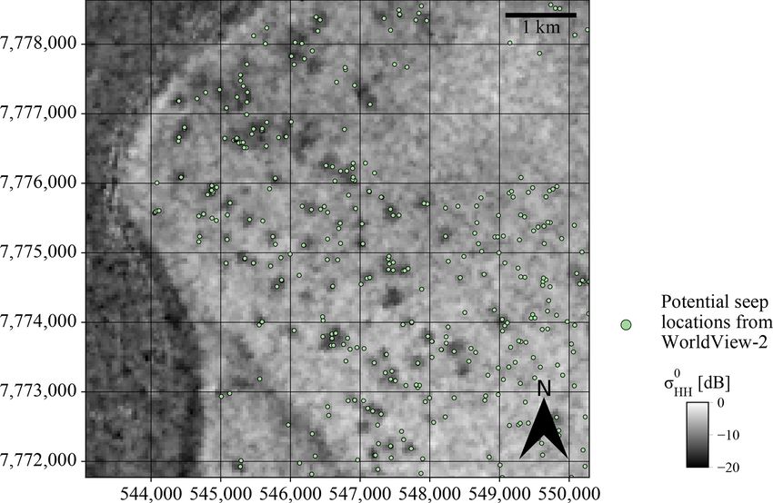
1916 G. Pointner et al.: Mapping potential signs of gas emissions in ice of Lake Neyto
from the EW and IW classification results, we estimate the Table 4. Metrics for the comparison between binary classifications
total number of pixels in the negative class (regular float- of Sentinel-1 EW and Sentinel-1 IW acquisitions on consecutive
ing lake ice) to be about 1 order of magnitude larger than days. A total of 10 pairs of EW and IW acquisitions were used.
the total number of pixels in the positive class (anomalies)
in the validation dataset (Table 2), so class imbalance is F1-score binary 0.80
clearly the case here and simple accuracy measures should F1-score macro 0.89
be avoided (Chicco and Jurman, 2020). We faced a simi- Matthews correlation coefficient 0.78
Cohen’s kappa coefficient κ 0.78
lar situation of imbalance when looking at the number of
pixels classified positively over time; i.e. there is a signifi-
cant difference between the number of pixels classified posi-
tively in February and the number of pixels classified pos- 5 Results
itively in May, for example. So, we argue that averaging
metrics over the 10 points in time (Table 2) cannot be rep- An example of classification results from Sentinel-1 EW and
resentative for the classification method either. We propose IW imagery acquired on consecutive dates is given in Fig. 4
to calculate binary metrics which are suitable in the case of (HH-polarisation and VV-polarisation bands are shown in
imbalanced classes on all classified pixels in the validation Fig. 4a and b, respectively). Anomalies are characterised by
dataset, together. Specifically, we calculated F1 scores (Dice, similar contrast and similar extents in the two acquisitions.
1945; Sørensen, 1948), the Matthews correlation coefficient Table 4 shows the metrics calculated from the comparison
(Matthews, 1975) and Cohen’s kappa coefficient κ (Cohen, between classifications from EW and IW modes in the val-
1960). F1 scores are generally calculated per class. We give idation set. κ and the Matthews correlation coefficient have
two versions of F1 scores here, one being the F1-score bi- the same value (0.78); the F1-score binary is slightly higher
nary, which is calculated for the positive class (anomalies) (0.80), and the value of the F1-score macro is 0.89.
only, and one being the F1-score macro, which is the average As described in Sect. 4.3, the validation dataset consists of
of the F1 scores of the positive and negative class. 10 pairs of Sentinel-1 images acquired in EW and IW modes
In order to compare backscatter levels among modes and on consecutive dates. Several statistics were calculated from
polarisation channels, we also used the data from this valida- the validation set to describe backscatter levels. Boxplots of
tion dataset because of the short time interval between acqui- σ 0 for the positive class (anomalies) and negative class (reg-
sitions in the two modes. We calculated mean σ 0 per class ular floating lake ice) are shown in Fig. 5 for all polarisations
and date, took the difference between the means per class for and acquisition dates in the validation set. The temporal aver-
each acquisition date, and calculated the mean of these differ- ages of the differences between mean σ 0 of the positive and
ences over time. Further, we calculated the mean σ 0 for the negative class on the single acquisition dates are 4.9 dB for
positive class on single dates and averaged it over time. All the EW mode in HH polarisation, 6.0 dB for the EW mode in
calculations were performed separately for each polarisation HV polarisation, 5.4 dB for the IW mode in VV polarisation
channel. and 7.2 dB for the IW mode in VH polarisation.
The temporal averages of mean σ 0 of the positive class
4.4 Summary of the most important methodological (anomalies) on single acquisition dates are −12.2 dB for the
steps EW mode in HH polarisation, −25.9 dB for the EW mode in
HV polarisation, −14.1 dB for the IW mode in VV polarisa-
A flow chart depicting the most important processing, se- tion and −25.4 dB for the IW mode in VH polarisation.
lection and analysis steps associated with Sentinel-1 and Figure 6a shows an example of detected holes in the
WorldView-2 data is shown in Fig. 3. Sentinel-1 EW and lake ice of Lake Neyto on a true-colour composite of the
IW data were both pre-processed and classified using a sim- WorldView-2 acquisition from 22 May 2016, and Fig. 6b
ilar methodology. Classification results of IW and EW data shows examples of mapped holes from the watershed seg-
acquired on consecutive dates (Table 2) were used to calcu- mentation algorithm. Holes are clearly characterised by dark
late validation metrics. Polygons of detected holes deduced tones surrounded by regions of higher reflectance.
from the blob detection and subsequent watershed segmen- The blob-detection algorithm yielded locations of
tation on the green band of the pan-sharpened WorldView-2 718 holes. Out of 718 hole polygons deduced by using
image acquired on 22 May 2016 were used to calculate statis- the watershed segmentation, 10 had to be excluded by the
tics of the hole area. Detected locations of holes as produced application of the area threshold (compare to Sect. 4.2.2).
by the blob-detection algorithm were visually and quantita- Figure 7 shows a histogram of hole areas from the remaining
tively compared to single Sentinel-1 EW acquisitions and 708 hole polygons. The majority of holes are characterised
associated anomaly classification results from 16 May and by an area smaller than 5 m2 ; the median is 4.00 m2 . Few
7 April 2016. holes with areas larger than 50 m2 were identified.
The locations of the 718 detected holes (points, poten-
tial seep locations) from the WorldView-2 image acquired
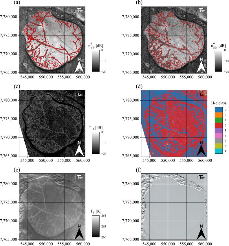
The Cryosphere, 15, 1907–1929, 2021 https://doi.org/10.5194/tc-15-1907-2021G. Pointner et al.: Mapping potential signs of gas emissions in ice of Lake Neyto 1917 Figure 3. Workflow of main processing, selection and analysis steps associated with Sentinel-1 and WorldView-2 imagery in this study. Figure 4. Example of Sentinel-1 EW and IW acquisitions taken 1 d apart and classification outcomes of backscatter anomalies. (a) Sentinel-1 EW HH-polarised acquisition from 24 May 2019. (b) Sentinel-1 IW VV-polarised acquisition from 25 May 2019. Red outlines represent polygon outlines from vectorised raster classification maps. CRS: WGS 84 / UTM zone 42N. on 22 May 2016 and the Sentinel-1 HH-polarised image 7 April 2016, taken more than a month earlier than the image acquired on 16 May 2016 with the outlines of classified in Fig. 8. A detailed view of the northwestern part of Lake backscatter anomalies (polygons) are shown in Fig. 8. Of Neyto is shown. A relationship between many locations of the 718 detected holes, 71 % lie within the polygons deduced holes and backscatter anomalies with a smaller spatial extent from the Sentinel-1 classification result. The mean minimum can be identified. Maximum and minimum air temperatures distance between the points and the polygons is 38 m (if a on 22 May 2016 were 1.2 and −2.0 ◦ C, respectively, accord- point lies within a polygon, the distance is zero). The median ing to the ERA5 data (Hersbach et al., 2018). Apart from distance of all points lying outside the polygons is 67 m. 1 April and 3 d from 22 to 24 April, maximum air tempera- Interesting spatial relationships can also be identified ture remained below 0 ◦ C until 16 May 2016 (Hersbach et al., when comparing the locations of detected holes to Sentinel- 2018). 1 imagery acquired earlier in the same year. Figure 9 shows The automated classification approach on Sentinel-1 EW the same locations of detected holes deduced from the data makes it possible to compose time series of areas of WorldView-2 image acquired on 22 May 2016 as in Fig. 8 backscatter anomalies and compare them to time series of on top of a Sentinel-1 EW HH-polarised acquisition from minimum and maximum air temperatures over the years https://doi.org/10.5194/tc-15-1907-2021 The Cryosphere, 15, 1907–1929, 2021
1918                                          G. Pointner et al.: Mapping potential signs of gas emissions in ice of Lake Neyto

Figure 5. Boxplots of σ 0 for the positive class (backscatter anomalies) and negative class (regular floating lake ice) for all polarisations
(HH, HV, VV, VH) and all 10 acquisition dates in the validation set. The means are represented by triangles. Dates are given in the format
year–month–day.

2015 to 2019 (Fig. 10a–e). A steady increase in area of                  lap often increases when the air temperatures approach or
backscatter anomalies in late winter and spring is evident.              exceed 0 ◦ C.
The maximum extent of backscatter anomalies was espe-                       The results of the ALOS PALSAR-2 polarimetric analyses
cially high in 2019, when on the last useful acquisition                 can be directly compared to Sentinel-1 acquisitions in EW
date, its area was approximately half of the whole lake area             and IW modes (Fig. 11) and to Landsat 8 brightness tem-
(Fig. 10; compare also to Fig. 4a). Maximum air tempera-                 perature and surface reflectance data acquired in April 2015.
ture often approaches or slightly exceeds 0 ◦ C throughout the           As expected, backscatter is clearly lower in anomaly zones
analysis periods. Days where maximum air temperatures ex-                than for regular floating lake ice in both Sentinel-1 IW
ceed 0 ◦ C are shown by the dashed lines in Fig. 10. In order to         VV-polarised (Fig. 11a) and Sentinel-1 EW HH-polarised
assess the expansion of anomaly regions, the fraction of over-           (Fig. 11b) images. The T11 component of the coherency ma-
lap between anomaly regions on consecutive dates is shown                trix, which is related to the magnitude of surface scattering
in brown (area of intersection between classified anomaly re-            (Engram et al., 2013), interestingly indicates lower backscat-
gions on the timestamp indicated and that of the previous                ter from regular floating lake ice compared to anomaly zones
timestamp, divided by area of the classified anomaly regions             in the L band (Fig. 11c). The polarimetric classification
at the previous timestamp). The fraction is especially high              (Fig. 11d) shows that regular floating lake ice largely falls in
during the last observation dates in the years concerned. In             region 6 (random surface), while anomaly regions mainly fall
order to avoid division by zero, the graphs were only calcu-             in region 9 (Bragg surface) of the H -α plane (Lee and Pot-
lated for the time period after zero anomalies were detected             tier, 2009). The brightness temperature in anomaly regions
for the last time in the years concerned. The fraction of over-          is approximately 1 to 2 K higher than in the rest of the lake
                                                                         (Fig. 11e), while the snow surface appears rather homoge-

The Cryosphere, 15, 1907–1929, 2021                                                           https://doi.org/10.5194/tc-15-1907-2021
G. Pointner et al.: Mapping potential signs of gas emissions in ice of Lake Neyto 1919
Figure 8. Comparison of detected holes (potential seep locations,
green points) from WorldView-2 imagery acquired on 22 May 2016
and backscatter anomalies (red outlines) from a Sentinel-1 scene
acquired on 16 May 2016 on top of the HH-polarisation band of
the same scene. The blue outline shows the analysis extent that is
determined by the extent of the WorldView-2 image and the lake
and shelf masks. CRS: WGS 84 / UTM zone 42N.
Figure 6. Examples of hole detection and classification results in
lake ice of Lake Neyto on WorldView-2 true-colour composites ac-
quired on 22 May 2016. (a) Examples of detected holes (red circles)
from the blob-detection method. Radii of circles are scaled propor-
tionally to the standard deviation of the LoG kernel that detected
the respective blob, enlarged for the visualisation. (b) Mapped
holes (red outlines) from the watershed segmentation method. CRS:
WGS 84 / UTM zone 42N.
Figure 9. Comparison of detected holes (potential seep locations,
green dots) from WorldView-2 imagery acquired on 22 May 2016
on top of the HH-polarisation band of a Sentinel-1 scene acquired
on 7 April 2016 showing backscatter anomalies at an early stage of
development. CRS: WGS 84 / UTM zone 42N.
neous but also shows very small differences in anomaly re-
gions in the true-colour composite of surface reflectance in
Fig. 11f.
6 Discussion
Validation metrics from the comparison between classifica-
tion results from EW and IW modes are relatively high, with
similar values for the F1-score binary (0.80), the Matthews
Figure 7. Histogram of hole areas from 708 hole polygons de- correlation coefficient (0.78) and Cohen’s κ (0.78). The F1-
duced from the watershed segmentation algorithm applied to the score macro (average of F1 scores for the positive and neg-
WorldView-2 image acquired on 22 May 2016. ative class) is higher than the F1-score binary because of a
significantly higher F1 score for the negative class, for which
https://doi.org/10.5194/tc-15-1907-2021 The Cryosphere, 15, 1907–1929, 2021You can also read