Meteor Shower Modeling: Past and Future Draconid Outbursts
←
→
Page content transcription
If your browser does not render page correctly, please read the page content below
Meteor Shower Modeling: Past and Future Draconid Outbursts

                                                  A. Egala,b,c,∗, P. Wiegerta,b , P. G. Browna,b , D. E. Moserd , M. Campbell-Browna,b , A. Moorheade , S.
                                                                                            Ehlertf , N. Moticskae,g
                                                    a Department    of Physics and Astronomy, The University of Western Ontario, London, Ontario N6A 3K7, Canada
                                                b Centre   for Planetary Science and Exploration, The University of Western Ontario, London, Ontario N6A 5B8, Canada
                                               c IMCCE, Observatoire de Paris, PSL Research University, CNRS, Sorbonne Universités, UPMC Univ. Paris 06, Univ. Lille
                                                   d Jacobs Space Exploration Group, NASA Meteoroid Environment Office, Marshall Space Flight Center, Huntsville, AL

                                                                                                        35812 USA
                                                               e NASA Meteoroid Environment Office, Marshall Space Flight Center, Huntsville, AL 35812 USA
                                                f Qualis Corporation, Jacobs Space Exploration Group, NASA Meteoroid Environment Office, Marshall Space Flight Center,

                                                                                                 Huntsville, AL 35812 USA
arXiv:1904.12185v1 [astro-ph.EP] 27 Apr 2019

                                                                              g Embry-Riddle Aeronautical Univeristy, Daytona Beach, FL, USA

                                               Abstract
                                               This work presents numerical simulations of meteoroid streams released by comet 21P/Giacobini-Zinner
                                               over the period 1850-2030. The initial methodology, based on Vaubaillon et al. (2005), has been updated
                                               and modified to account for the evolution of the comet’s dust production along its orbit. The peak time,
                                               intensity, and duration of the shower were assessed using simulated activity profiles that are calibrated to
                                               match observations of historic Draconid outbursts. The characteristics of all the main apparitions of the
                                               shower are reproduced, with a peak time accuracy of half an hour and an intensity estimate correct to
                                               within a factor of 2 (visual showers) or 3 (radio outbursts). Our model also revealed the existence of a
                                               previously unreported strong radio outburst on October 9 1999, that has since been confirmed by archival
                                               radar measurements. The first results of the model, presented in Egal et al. (2018), provided one of the best
                                               predictions of the recent 2018 outburst. Three future radio outbursts are predicted in the next decade, in
                                               2019, 2025 and 2029. The strongest activity is expected in 2025 when the Earth encounters the young 2012
                                               trail. Because of the dynamical uncertainties associated with comet 21P’s orbital evolution between the
                                               1959 and 1965 apparitions, observations of the 2019 radio outburst would be particularly helpful to improve
                                               the confidence of subsequent forecasts.
                                               Keywords: Meteors, Comet Giacobini-Zinner, dust, dynamics

                                               1. Introduction

                                                  The October Draconid shower (009 DRA) is an autumnal meteor shower known to episodically appear
                                               around the 9th of October since 1926. The Draconid shower, with apparitions irregular in time and intensity,
                                               has challenged the forecasts of modelers since its discovery. Its parent body is the Jupiter-family comet
                                               21P/Giacobini-Zinner, discovered in 1900, which has an erratic and highly perturbed orbit (Marsden and
                                               Sekanina, 1971). The Draconid annual activity is usually barely perceptible (with a rate of a few visual
                                               meteors per hour), but the stream occasionally produces strong outbursts and storms (up to ten thousand
                                               meteors per hour) that are not directly correlated with the past geometrical configuration between the Earth
                                               and the parent comet (Egal et al., 2018). In addition, some showers were observed by naked-eye witnesses
                                               or using video devices, while other outbursts (e.g. 2012) were caused by small meteoroids only detectable
                                               by radar instruments (Ye et al., 2014).

                                                 ∗ Corresponding author
                                                   Email address: aegal@uwo.ca (A. Egal)

                                               Preprint submitted to Elsevier                                                                           April 30, 2019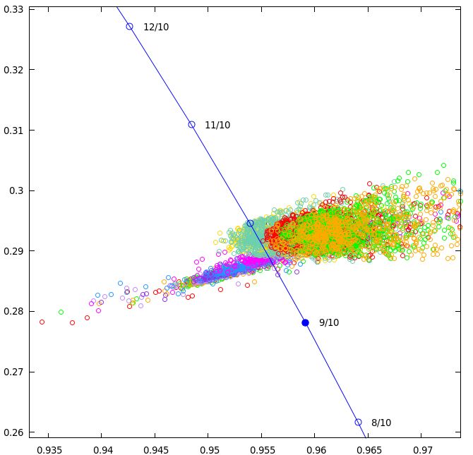
Previous attempts to predict upcoming Draconid activity have had mixed success. Of the nine historic
outbursts of the shower (1926, 1933, 1946, 1952, 1985, 1998, 2005, 2011 and 2012), five were expected
(1926, 1946, 1985, 1998 and 2011) and predictions of three events correctly estimated the peak time with
an accuracy better than two hours. In 1946 the maximum activity occurred close to the descending node of
the comet, simplifying timing estimates. Reznikov (1993) accurately predicted the shower return in 1998,
caused by an encounter with the meteoroid stream ejected in 1926. More recently, a successful peak time
prediction concerned the 2011 outburst. Numerical simulations of meteoroid streams ejected from 21P
conducted by different authors estimated a maximum activity around 20h UT and a secondary peak around
17h on October 8 2011 (Watanabe and Sato, 2008; Vaubaillon et al., 2011); the existence of both peaks was
indeed confirmed by independent observation campaigns (e.g. McBeath, 2012; Trigo-Rodrı́guez et al., 2013;
Kac, 2015).
    If different models provided an accurate prediction of the 2011 apparition date, they also led to the
first reasonable estimate of the outburst’s strength. The activity of a shower, usually characterized by the
zenithal hourly rate (ZHR) parameter (i.e. the number of meteors a single observer would see during an hour
under ideal conditions), is a quantity that is hard to foresee. To our knowledge, no real intensity predictions
were performed for Draconid outbursts prior to the 1998 apparition. The first attempt of Kresák (1993) to
estimate the strength of the shower outburst in 1998, expected to be lower than the one occuring in 1985,
underestimated the 1998 shower’s intensity by a factor of ten.
    In 2011, ZHR estimates of the main peak ranged from 40-50 (Maslov, 2011) to 600 (Watanabe and Sato,
2008; Vaubaillon et al., 2011), with intermediate activity predictions reaching storm level (ZHR of 7000
in Sigismondi, 2011). Numerous observations of the 2011 Draconids estimated a ZHR between 300 (Kero
et al., 2012; McBeath, 2012) and 400-460 (Trigo-Rodrı́guez et al., 2013; Kac, 2015). Among the wide range
of ZHR predictions for 2011 published in the literature, some were in good agreement with the observations
(Watanabe and Sato, 2008; Vaubaillon et al., 2011). This success could have settled the question of Draconid
forecasts using numerical simulations. However, a completely unexpected radio storm reaching a ZHR of
9000±1000 meteors per hour was observed one year later (Ye et al., 2014), highlighting the need to improve
the intensity predictions of meteor showers.
    The motivation underlying the present work was therefore to be able to predict not only the date and
time of appearance of a Draconid shower, but to also provide a quantitative estimate of its intensity with
relative confidence. Since the numerical modeling of meteoroid streams ejected from the parent comet is
the only efficient tool to predict such a shower, we performed simulations of the {21P, Draconid} complex
using the model of Vaubaillon et al. (2005). For the first time, we simulated ZHR profiles for each year of
predicted enhanced Draconid activity and compared them with the available observations. The simulated
profiles were then calibrated against observations of the timing, activity profile and strength of historic
Draconid outbursts to reinforce the reliability of future forecasts. This work presents the implementation
and results of our meteoroid stream modeling, applied specifically to the Draconid shower. The structure of
the paper is comprised of four main parts, some of which consist of multiple sections.

   • In Section 2, we detail the main characteristics of the historic Draconid outbursts observed between
     1926 and 2012. Because the Draconids were widely analyzed by multiple observers using different
     instruments, the literature has a wide variety of information relating to the shower. For each event,
     we tried to highlight the conclusions shared by the highest number of authors or the best documented
     reports.
   • Sections 3, 4 and 5, together with Appendices A, B & C, describe in detail the implementation
     and interpretation of the new meteoroid stream model used here to reproduce or predict past and
     future Draconid occurrences (Model I). In section 6, we offer a succinct summary of the independently
     developed NASA Meteoroid Environment Office’s MSFC meteoroid stream model, used to validate
     Model I.
   • Section 7 presents the performance of Model I in reproducing the main visual and radio outbursts
     observed between 1933 and 2012, in terms of years of appearance and shower time, strength, and
     duration. A comparison between our simulations and observations of the previously unreported 1999
                                                      2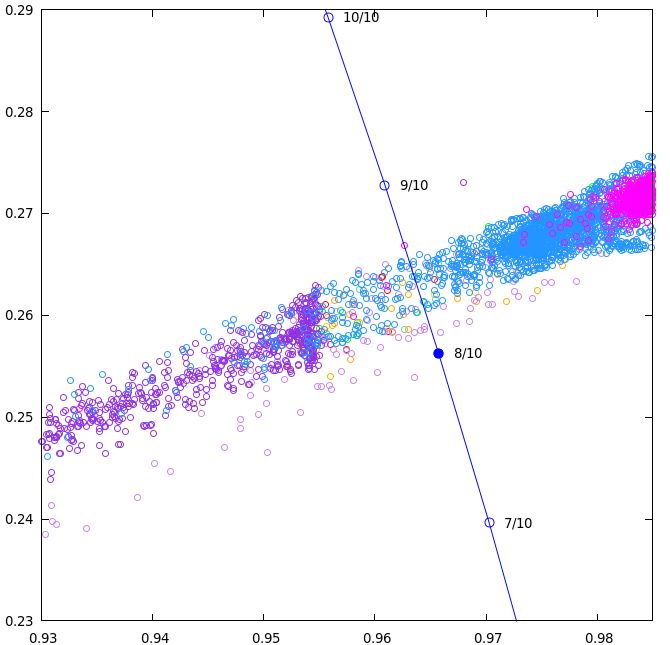
radio outburst, revealed by our model, is also presented. An initial comparison between the 2018
     prediction performed in Egal et al. (2018) and preliminary visual and radio observations of this recent
     outburst, shared by the International Meteor Organization (IMO), is given in section 8. The simulated
     activity profiles presented in these sections form the main validation of the approach employed by
     Model I.

   • Finally, Section 9 details our predictions for three potential radio outbursts expected in the next decade
     (2019, 2025 and 2029). The reliability of this forecast, intrinsically correlated to Model I’s accuracy,
     is discussed in Section 10.

2. Draconid observations

    The Draconids are known to have produced two storms observed optically in 1933 and 1946, as well as
more moderate shower outbursts in 1926, 1998, and 2011. Other Draconid outbursts were detected mainly
by radar techniques in 1952, 1985, and 2005, in addition to a radio storm in 2012. Very low activity from the
shower was reported in 1972 instead of the intense outburst/storm that was originally predicted (McIntosh,
1972; Hughes and Thompson, 1973).
    In this work, we classify the Draconid apparitions into three categories: the outbursts which were visu-
ally observed or recorded using optical instruments (“visual outbursts”), the showers mainly observed by
radio/radar devices (“radio outbursts”), and weak or poorly documented showers.

2.1. Established visual outbursts
1933
   The 1933 storm occurred on October 9 around 20h15 UT (Watson, 1934), for a total duration of about
4h30 (R. Forbes-Bentley in Olivier, 1946). ZHR estimates of the shower are very disparate and vary from
around 5400 (Watson, 1934) to 10 000 (Jenniskens, 1995) and even 30 000 (Olivier, 1946; Cook, 1973).

1946
   The 1946 storm was by visual, photographic, and radar techniques mainly in Europe and North America.
The shower peaked around 3h40-3h50 UT on October 10, and lasted 3 to 4 hours (Lovell et al., 1947; Kresak
and Slancikova, 1975). Again, ZHR estimates in the literature vary between 2000 (Hutcherson, 1946) and
6800 (Kresak and Slancikova, 1975) or 10 000 (Jenniskens, 1995).

1998
   The 1998 outburst appeared on October 8, peaking around 13h10 UT (Koseki et al., 1998; Arlt, 1998;
Watanabe et al., 1999) although Šimek and Pecina (1999) indicated a maximum around 13h35 UT. The
total duration was about 4h (Watanabe et al., 1999), and the maximum ZHR reached 700 to 1000 meteors
per hour (Koseki et al., 1998; Arlt, 1998; Watanabe et al., 1999).

2011
    Following the concordant predictions of an outburst in 2011, the Draconids were observed on October
8 by many teams with many different observational techniques (radar, video, photography, visual). The
main peak occurred around 20h-20h15 UT, for a total duration of about 3 to 4 hours and a maximum ZHR
estimate varying from 300-400 to 560 (Toth et al., 2012; Kero et al., 2012; Koten et al., 2014; Molau and
Barentsen, 2014; McBeath, 2012; Trigo-Rodrı́guez et al., 2013; Kac, 2015).

                                                      3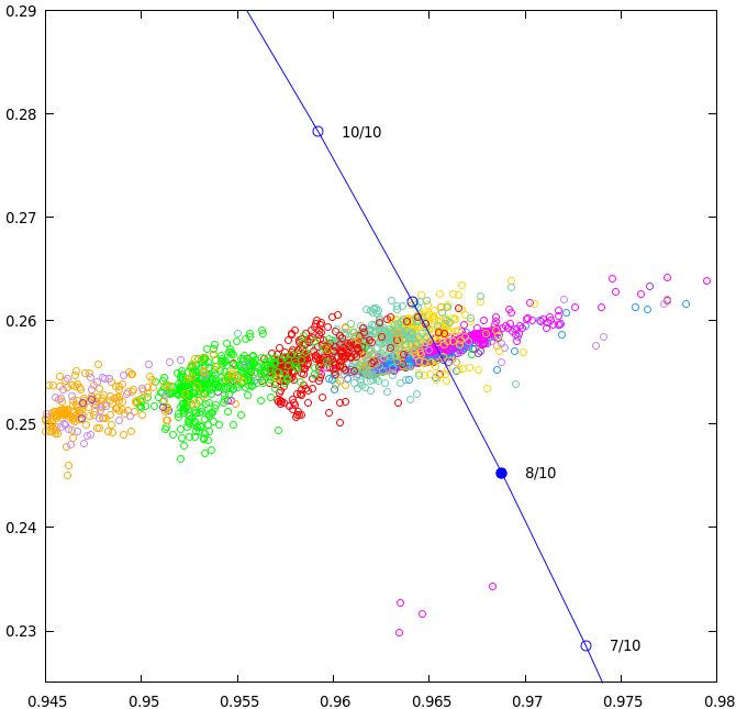
2.2. Established radio outbursts
1985
   The 1985 peak occurred on October 8 between 9h25 and 9h50 (Chebotarev and Simek, 1987; Simek, 1994),
probably around 9h35 UT (Lindblad, 1987; Sidorov et al., 1994). The observed shower duration varies from
3h (Lindblad, 1987; Mason, 1986) to 4h30 (Sidorov et al., 1994). An equivalent ZHR is estimated to be from
around 400-500 (Lindblad, 1987; Simek, 1994) to possibly as high as 2200 (Mason, 1986). In agreement with
the radio measurements, visual observations carried out in Japan in 1985 confirmed a ZHR higher than 500
shortly before 10h UT on October 8 (Koseki, 1990).

2005
    The unexpected 2005 radio outburst was detected on October 8 around 16h05 UT (Campbell-Brown
et al., 2006). The end of the shower was missed by radar, while the beginning was not observed using visual
techniques (Koten et al., 2007); producing only a lower limit of 3h for the shower duration. The equivalent
ZHR was estimated to be around 150 (Campbell-Brown et al., 2006).

2012
   The 2012 storm happened on October 8 at 16h40, for a peak duration of about 2h and an equivalent
ZHR of 9000 (Ye et al., 2014). Fujiwara et al. (2016) measured a total duration of the shower of about 3
hours, with a peak time occurring between 16h20 and 17h40 UT.

2.3. Weak or controversial shower returns
1926
   The meteor activity observed by visual observers in October 1926 allowed the shower to be linked to
comet 21P/Giacobini-Zinner. From 36 meteors observed between 20h20 and 23h20 (G.M.T) on October 9
1926, a ZHR of about 20 meteors per hour was estimated (Denning, 1927). A Draconid fireball, observed
around 22h16 (G.M.T) that night, impressed the observers by leaving a persisting train during half an hour
(Denning, 1927; Fisher, 1934).

1952/1953
   Draconid activity was noticed by the Jodrell Bank radar on October 9 1952, with a maximum ZHR of
170-180 around 15h 40-50 min UT (Davies and Lovell, 1955). The shower duration was approximately 3
hours. The apparition of Draconid meteors the following year, in 1953, is controversial; no enhanced activity
was detected by the Jodrell Bank radar at any time within 12 hours of the expected maximum time (Jodrell
Bank, 1953), while other authors suggest some weak activity (Jenniskens, 2006).

1972
    Due to the favorable geometrical configuration between the comet and the Earth, a potentially strong
outburst/storm was expected on October 8 1972. However no significant activity was observed (Millman,
1973). Radar observations revealed a diffuse component of the shower, with a weak maximum activity at
October 8.2±0.3 (Hughes and Thompson, 1973). Radio observations carried in Japan might however argue
for a stronger radio activity, with a peak of 84 meteors detected in a 10 minute interval around 16h10 UT
on October 8 1972 (Marsden, 1972).

   Having summarized the major observational features of the Draconids over the last century, our next
goal is to reproduce the years of recorded activity, shower timing, strength and activity profile from a model.
We attempt to do this employing a model with the fewest number of tunable parameters which also provides
good fits to the most robustly determined characteristics of the shower.

                                                      4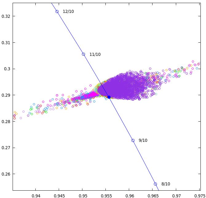
3. Model I - Simulations

3.1. 21P/Giacobini-Zinner
    Comet 21P/Giacobini-Zinner was observed for the first time by M. Giacobini in 1900, and identified
again by E. Zinner in 1913. Since its discovery, at least 16 apparitions of the comet have been observed
and numerous orbital solutions produced. 21P is a typical Jupiter-family comet (JFC), with a period of
approximately 6.5 years and a current perihelion distance of 1.03 au. The comet has suffered multiple
close encounters with Jupiter through its history, resulting in our simulations in a global reduction of its
semi-major axis and increase of its eccentricity in 400 years. The comet’s motion has also been affected by
sudden and significant variations in the nongravitational forces (NGF) induced by its outgassing, causing
21P to be classified as an “erratic” comet (Sekanina, 1993). A particular discontinuity in the transverse
NGF coefficient between 1959 and 1965 dramatically modified 21P’s orbit (Yeomans and Chodas, 1989). The
gas and dust production of the comet used to peak after perihelion before this epoch, while the maximum
outgassing has occurred pre-perihelion since then (Sekanina, 1985; Blaauw et al., 2014).

3.1.1. Ephemeris
    Several studies have tried to reproduce the comet’s dynamical evolution during the 20th century, in
particular a significant discontinuity in its orbital evolution observed between 1959-1965. Despite a moder-
ately close approach with Jupiter in 1958, the gravitational influence of the giant planet did not seem to be
responsible for the orbital variations observed around 1959 (Yeomans, 1971, 1972).
    Sekanina (1985); Królikowska et al. (2001) were able to explain the NGF evolution of 21P by considering
the precession of the comet’s spin axis. However, Sekanina’s model yielded unrealistic values of the comet’s
oblateness and rotation period (Yeomans, 1986; Królikowska et al., 2001), while the Królikowska analysis
required many additional parameters derived from observations (e.g. relative times between the maximum
activity and the perihelion passage for different apparitions) to correctly link all the comet’s apparitions.
Another independent explanation for the erratic orbital evolution of 21P could be the activation of discrete
source regions at the surface of the comet, at specific locations and for a certain duration (Sekanina, 1993).
    In their current state, neither of these models permits the comet’s ephemeris to be reproduced without
involving a detailed knowledge of its past apparitions; for our study, we therefore decided to rely directly
on the observations. The comet’s motion at each apparition is integrated from an orbital solution provided
by the JPL Small Body Data Center1 , with an external time step of 1 day and considering the asymmetric
non-gravitational forces model of Yeomans and Chodas (1989).

3.1.2. Integration period
    Because of the 1959 orbital evolution discontinuity, we chose to build the ephemeris of each apparition of
the comet from the closest available orbital solution, and not from the most recent measured orbit of 21P.
However, older observations of 21P (prior to 1966) were determined with less accuracy, which may reduce
the reliability of our integrations. In order to evaluate the impact of this approach on the comet ephemeris,
we compared the trajectories integrated from 15 distinct orbital solutions of 21P obtained for the years 1900,
1913, 1926, 1933, 1940, 1946, 1959, 1966, 1972, 1979, 1985, 1992, 1998, 2006, and 2013.
    Figure 1 illustrates the evolution with time of the minimum, maximum, and average similarity criterion
DSH (Southworth and Hawkins, 1963) for each pair of trajectories obtained (left panel). The middle
panel presents the variations of the descending node’s heliocentric distance for each initial orbital solution
considered. The right panel was obtained by considering the same initial orbit (2006 solution) but integrating
the trajectory with different nongravitational force models (no NGF, symmetric outgassing, and asymmetric
outgassing, respectively).
    In Figure 1, we observe a slight increase of the DSH around 1960. The DSH evolution before this date
coincides with the dispersion noticeable in the node distances plots. The first significant dispersion of the
orbits occurs in 1898, as a consequence of a close encounter with Jupiter. Earlier close approaches with

  1 https://ssd.jpl.nasa.gov/sbdb.cgi

                                                      5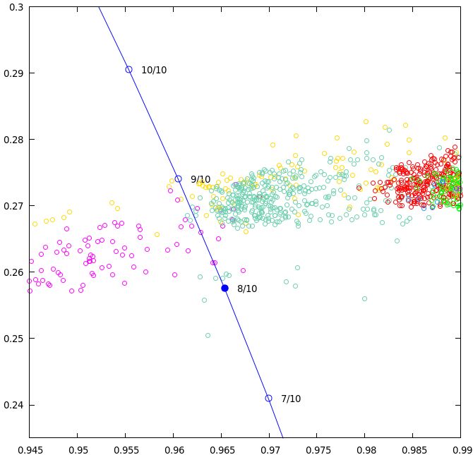
0.6                                                                                  1.9                                                                                   1.9
                                     DSH min                                                                                    2013                                                                    Asymmetric NGF
                                                                                                                                2006
                                    DSH mean                                               1.8
                                                                                                                                1998
                                                                                                                                                                                 1.8                     Symmetric NGF

                                     DSH max

                                                         Node heliocentric distance (au)

                                                                                                                                               Node heliocentric distance (au)
      0.5                                                                                                                       1992                                                                            No NGF
                                                                                           1.7                                  1985                                             1.7
                                                                                                                                1979
                                                                                                                                1972
                                                                                           1.6                                                                                   1.6
                                                                                                                                1966
      0.4
                                                                                                                                1959
                                                                                           1.5                                  1946                                             1.5
                                                                                                                                1940
DSH

                                                                                                                                1933
      0.3                                                                                  1.4                                                                                   1.4
                                                                                                                                1926
                                                                                                                                1913
                                                                                           1.3                                  1900                                             1.3

      0.2                                                                                                                   1900
                                                                                           1.2                               to                                                  1.2
                                                                                                                            2013

                                                                                           1.1                                                                                   1.1
      0.1

                                                                                            1                                                                                     1

       0                                                                                   0.9                                                                                   0.9
        1700   1750   1800   1850   1900   1950   2000                                       1700   1750   1800   1850   1900    1950   2000                                       1700   1750   1800   1850    1900   1950   2000

                             Year                                                                                 Year                                                                                   Year

Figure 1: Left panel: time evolution of the minimum, maximum, and mean DSH between each pair of orbits determined
from 15 distinct initial orbital solutions. Middle panel: heliocentric distance of the descending nodes of 21P along time, for
15 initial orbital solutions ranging from 1900 to 2013. Right panel: heliocentric distance of the descending node for different
nongravitational forces models.

Jupiter in 1815 and 1732 also disperse the orbits. From this analysis, we conclude that the orbital solution
selected for the comet ephemeris computation should not influence the prediction of the meteor showers
caused by trails ejected after the comet’s discovery. For older streams, however, the initial integration epoch
has a significant impact on the comet ephemeris, and hence on the meteoroid stream generated. Since the
Draconids are often associated with young material (Lindblad, 1987; Wu and Williams, 1995; Vaubaillon
et al., 2011), our integrations were limited to the 1850-2030 period. If any interpretation of the contribution
of trails ejected prior to 1898 needs to be carefully conducted, their influence on our predictions is negligible.
Particles ejected over the 1850-1898 period were only simulated for comparison of the nodal footprints of
the simulated Draconids with previous works (e.g. with Vaubaillon et al., 2011).

3.1.3. Physical properties
    The lack of direct imaging of 21P’s nucleus forces us to estimate certain physical properties needed for
our integrations. The radius of the nucleus of 21P is not well determined; estimates suggest it probably lies
between 1 and 2 km (Leibowitz and Brosch, 1986; Singh et al., 1997; Lamy et al., 2004; Pittichová et al.,
2008). By default, we consider a nucleus density of 400 kg m−3 and an albedo of 0.05 commonly assumed for
JFCs (Newburn and Spinrad, 1985; Landaberry et al., 1991; Hanner et al., 1992). The percentage of active
surface, unknown for 21P, is fixed to 20%. A summary of the model’s parameters is presented in Table 1.

3.2. Meteoroid streams
3.2.1. Ejection
    Particles are ejected at each simulation time step of the comet for heliocentric distances below 3.7 au
(Pittichová et al., 2008). Around 12.48 million dust particles were simulated over the period 1850-2020,
covering the size bins [10−4 , 10−3 ] m (10−9 , 10−6 ) kg: (160 000 particles per apparition), [10−3 , 10−2 ] m
(10−6 , 10−3 ) kg: (190 000 particles) and [10−2 , 10−1 ] m (10−3 , 1) kg: (130 000 particles). An additional
sample of 120 000 particles in each size bin was ejected at each comet apparition between 1852 and 2025,
and integrated until the year 2030 (9.72 million particles). In total, 22.2 million dust particles were simulated
over the period 1850-2030.
    The meteoroid density is assumed to be 300 kg m−3 , as determined by Draconid meteor observations
(Borovička et al., 2007). Simulated particles are isotropically ejected from the sunlit hemisphere of the
comet, with velocities determined by the Crifo and Rodionov (1997) model, which produces ejection speeds
most in accord with recent in situ cometary measurements (c.f. Appendix A).

                                                                                                                  6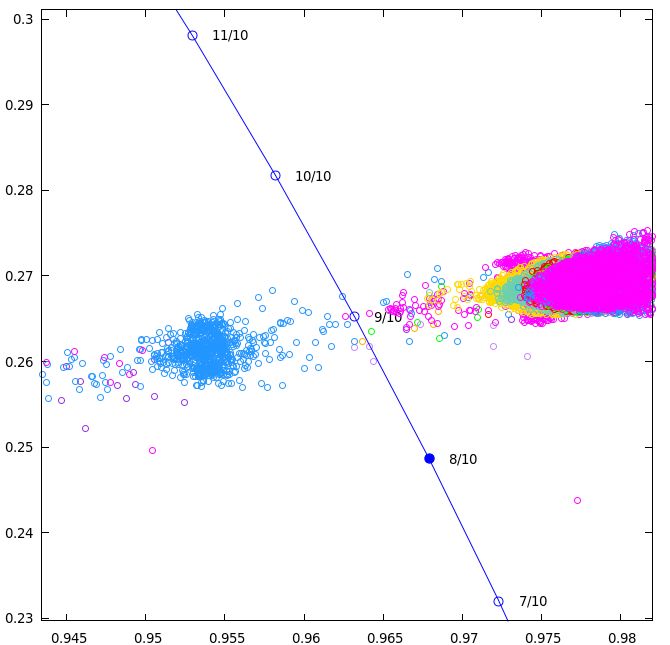
3.2.2. Integration
    The stream integration is performed in Fortran 90 using a 15th order RADAU integrator with a precision
control parameter LL of 12 (Everhart, 1985). The external integration step is fixed to one day and the internal
time steps are variable, allowing close encounters with planets to be dealt accurately. The gravitational
attraction of the Sun, the Moon, and the eight planets of the solar system as well as general relativistic
corrections are taken into account. Solar radiation pressure and Poynting-Robertson drag are also included.
The Yarkovsky-Radzievskii effect was neglected since the size of our simulated particles doesn’t exceed 10
cm (Vokrouhlický and Farinella, 2000).

3.2.3. Impact selection
    As a first selection, all particles that approach the Earth below a distance ∆X = Vr ∆T are considered
potential impactors, with Vr the relative velocity between the planet and the particle and ∆T a time
parameter depending on the shower duration. The length of a typical Draconid shower doesn’t exceed a few
hours; we consider for this study a conservative time interval of ∆T = 1 day and a distance threshold ∆X
of 1.15 × 10⁻² au. Potential impacting particles are, in a second step, individually integrated with a time
step of one minute, in order to precisely estimate the date and position of their closest approach with the
Earth.

                  Comet parameter                   Choice                      Reference
                  Shape                            Spherical
                  Diameter                           2 km                  Lamy et al. (2004)
                  Density                         400 kg m−3
                  Albedo                              0.05
                  Active surface                      20 %
                  Active below                       3.7 au             Pittichová et al. (2008)
                  Variation index γ1 , γ2           2.1, 7.3                   This work
                  K1                                 ∼ 100                     This work
                  Af ρmax                        ∼1600-1800 cm                 This work

                  Particle parameter                 Choice                     Reference
                  Shape                             Spherical
                  Size                           10−4 to 10−1 m
                  Density                          300 kg m−3          Borovička et al. (2007)
                  Ejection velocity model         “CNC” model         Crifo and Rodionov (1997)
                  Ejection rate                     each day
                  Nparticles / apparition           ∼ 840 000

           Table 1: Comet and meteoroid characteristics considered by Model I. See the text for more details.

4. Model I - Interpretation

    The primary goal of this work is to compare our simulated meteor showers to Draconid observations with
the goal of matching the peak date, peak intensity, duration and overall activity profiles of past showers.
Because of limited computational resources, the number of particles ejected in our model is not comparable to
the true number of meteoroids effectively released by comet 21P/Giacobini-Zinner. It is therefore necessary
to extrapolate from the comparatively finite number of simulated particles to the true number of particles
in the stream.
    Since the number of simulated particles that would physically impact the Earth is too small to derive
a reliable flux profile, we consider each particle that passes within a sphere S, centered on the Earth and

                                                           7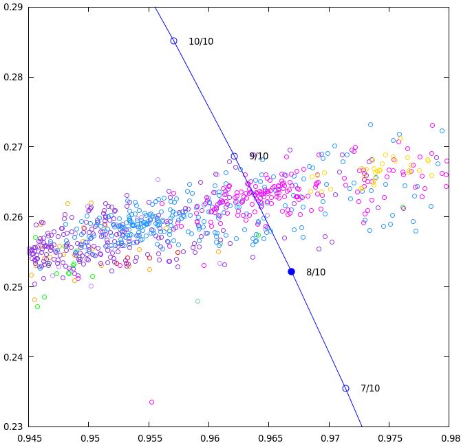
with a given radius Rs , as contributing to the shower. The Rs value must be smaller than the previous
∆X spatial criterion to exclude surrounding streams not producing any activity at the Earth. On the other
hand, Rs needs to be large enough to include a statistically useful sample of particles. The selection of the
Rs parameters for the Draconids simulations is discussed in Section 4.2.
Once particles are selected using the reduced distance criterion Rs , we assign to each impactor a weight
Ng which represents the scaling required to move from the small number of simulated meteoroids to the
true number which would be released by the comet in the same ejection circumstances.
4.1. Weights
The weighting process implemented here relies mainly on Vaubaillon et al. (2005), with some differences.
First, the evolution of the dust production for 21P/Giacobini-Zinner with the heliocentric distance rh is
extrapolated to each apparition from a photometric solution of the comet (cf. Appendix B). Second, the
gas and dust production are not assumed to be proportional to each other; this decoupling allows the gas
and dust production to evolve separately as a function of heliocentric distance (Sekanina, 1985). The main
hypotheses underlying the weighting solutions are:
1. The nucleus is spherical, homogeneous and composed of dust and water ice.
2. The dust production of the comet, represented by the Af ρ parameter (A’Hearn et al., 1984, cf.
Appendix B), evolves with the heliocentric distance rh . The gas-to-dust production ratio K is not
constant over rh .
3. The water molecules and the dust particles are ejected from the sunlit hemisphere of the nucleus, with
an intensity varying with the angle θ from the subsolar point.
4. The size distribution of the particles follows a power law of index u.
Details of the weighting computation are provided in Appendix C. For a given apparition of the comet
with a perihelion distance q, the number of particles ejected in all directions in the size bin [a01 , a02 ] during
time ∆t and around rh is found to be:
J∆t
0 0 1
Ng =K2 A1 (a1 , a2 ) · K1 ∆rh
2A(Φ) 2
Af ρmax h −γ(rh + ∆rh −q) i
∆r
−γ(rh − 2 h −q) (1)
− 10 2 − 10
γ ln(10)
γ =γ1 pre-perihelion and γ = γ2 post-perihelion
where:
- K2 is a tunable normalization coefficient constant over all the ejection conditions,
- A(Φ) is the nucleus albedo at phase angle Φ,
- Af ρmax is the maximum Af ρ obtained for a given apparition (ejection epoch),
- rh is the meteoroid heliocentric distance at the time of ejection (in au),
- q is the perihelion distance (au),
R a0
- A1 (a01 , a02 ) is shorthand for a02 adau , with a the particle radius (in m),
1
- K1 is a constant governing the Af ρ = f (rh ) evolution (fit parameter),
- γ is the Af ρ variation index, with γ = γ1 for pre-perihelion locations and γ = γ2 for post-perihelion
measurements, and
- J is a function of the ejection velocity and the minimal and maximal particle radii that can be ejected
from the comet (cf. Appendix C).
84.2. Flux and activity profile
The shower spatial number density Fs is estimated from the weighted number of particles entering the
sphere S over time. In this work, the sphere radius is fixed to Rs = V⊕ δt, with V⊕ the Earth’s heliocentric
velocity and δt a time parameter corresponding to the duration of the maximum activity of the shower.
For the most intense Draconid outbursts (e.g. 1946), most of the activity was contained within a one-hour
interval (Davies and Lovell, 1955; Kresak and Slancikova, 1975). For the main Draconid outbursts observed
visually (1933, 1946, 1998 and 2011), we then choose Rs = V⊕ × 1 h (Rs < 10 Earth radii). When the total
number of unweighted particles retained for the flux computation is lower than 15, δt is gradually increased
until either the number of particles exceeds 15 or δt is 6 hours (assumed to be the maximal duration of the
shower). The flux F of meteoroids is obtained by:
F = Fs · Vr (2)
with Vr the relative velocity between the Earth and the meteoroid stream. The zenithal hourly rate of the
shower is derived from F using Koschack and Rendtel (1990):
As F
ZHR = (3)
(13.1r − 16.5)(r − 1.3)0.748
where r is the measured population index of the shower and As an observer’s surface area of the atmosphere
at the ablation altitude (As ∼ 37200 km2 ).
4.3. Peak time estimate
The predicted peak date of the shower is determined by computing a weighted average of the simulated
activity profile. The presence of additional peaks, as well as the intensity and the duration of the shower,
are also derived from the ZHR evolution. In the case of simulated outbursts with a low number of particles
retained for the flux computation (δt > 1h), the resolution of the activity profiles may compromise the
validity of this approach. In such cases, the time of the peak maximum is taken to be the date of closest
approach between the Earth and the median location of the meteoroid streams (Vaubaillon et al., 2005).
5. Model I - Calibration
Before predicting any future Draconid showers, we need to determine the unknown parameters (K2 , u)
of the weighting function in Eq. 1 which best reproduce the past observed outbursts. The results are
particularly sensitive to the value of the size distribution index u of the meteoroids at ejection, since this
value influences the intensity and the shape of the activity profiles as well as the peak time estimate.
The calibration is first performed on the four strong visual showers of 1933, 1946, 1998, and 2011 and
then refined using the radio outbursts. The simulated ZHR profiles, derived from the meteoroid fluxes using
Equation 3 and a given population index r, are compared with the observations (see Figure 4 later). We
have chosen in the calibration process not to allow a variable population index, but instead adopt a fixed
value of r = 2.6 based on measurements of the 2011 (Toth et al., 2012; Kac, 2015) and potentially the 1933
shower (Plavec, 1957).
Our philosophy is that since any model can be improved when more free parameters are introduced,
we chose to limit the number of tunable parameters to the absolute minimum required. In doing this, we
decrease the match between the simulated and observed intensities of a specific shower in fixing r. However,
this allows us to determine the weighting solution that best reproduces all the outbursts with minimum
adjustable parameters, which we feel improves the robustness of the model shower prediction.
The best agreement between the simulated and the observed activity profiles for the four visual showers
was obtained for an ejecta size distribution index u of 2.9. This value differs from our previous published
estimate of 2.64 (Egal et al., 2018); differences between the two works are due to several factors. First, in
this work, we have increased the number of simulated particles by 75% and used a slightly different weighting
9solution which better reflects the observed Af ρ evolution of comet 21P. Second, the size distribution index
used here was determined considering two additional outbursts (1999 and 2018), not included in (Egal et al.,
2018).
Our calibrated value of u lies in the range of measurements performed for 67P (drifting from 2 beyond
2 au to 3.7 at perihelion, cf. Fulle et al., 2016). The associated cumulative mass index (smc = 0.63 for
u = 2.9) is somewhat lower than the value of 0.85 derived for comets 1P/Halley (McDonnell et al., 1987)
and 81P/Wild 2 (Green et al., 2004). Unfortunately, no such in situ measurement have been performed for
21P. Indirect estimates of u, inferred by meteor observations, are hampered by the variability of the observed
mass index changes with each apparition of the shower and even during an individual outburst (Koten et al.,
2014). In addition, because the orbital evolution of a meteoroid is size-dependent, a fundamental difference
between the size distribution index at the time of ejection and observation is not unexpected. Since no in
situ or indirect measurement of this parameter has been performed for 21P, the value of u = 2.9 will be
adopted through the rest of this study.
6. Model II - MSFC
For validation purposes, the Draconid streams simulated using Model I have been compared to an
independent meteoroid modeling performed by the NASA Meteoroid Environment Office (MEO). The MEO’s
MSFC Meteoroid Stream Model, similar to the model presented above, is detailed in Moser and Cooke (2004)
and Moser and Cooke (2008). The position and velocity of 21P/Giacobini-Zinner is taken from the 2006
orbital solution and ephemeris provided by JPL HORIZONS2 . The comet radius is assumed to be 1.7 km,
i.e. an average of Landaberry et al. (1991); Churyumov and Rosenbush (1991) and Newburn and Spinrad
(1989) measurements. 600 000 meteoroids are ejected at each apparition of the comet between 1594 and
2018, resulting in a total of about 35.4 million particles. Particles are released from the comet with a time
step of 1 hour, using the ejection model of Jones (1995) with a spherical cap angle of ejection of 30°. The
size of the particles are distributed uniformly over log β, where β ranges from 10−5 to 10−2 . β is defined as
the ratio between the forces due to the radiation pressure (Frad ) and the Sun’s gravity (Fgrav ), and can be
approximated by the following relation:
Frad 5.7 × 10⁻⁴
β= ' (4)
Fgrav aρ
with a and ρ respectively the radius (m) and density (kg m−3 ) of the particle. The selected β range of
10 to 10−2 corresponds to masses between 1 µg and 1 kg for the selected density of 1000 kg m−3 , and
−5
masses around ten times higher for the density of 300 kg m−3 considered by Model I.
The meteoroid integration is performed exactly as described in Section 3.2.2. Particles are retained as
potential impactors if they cross the Earth’s orbital plane within 0.01 au of the planet, and within ± 7
days of the expected shower peak. The time and intensity of the shower’s maximum activity are evaluated
through computation of an impact parameter (IP), defined as
R⊕ + hatmos
IP = (5)
D
where R⊕ is the Earth’s radius, hatmos the height of the atmosphere, and D the Earth-particle distance at
the time of nodal crossing. The impact parameter increases the weight of particles passing by the Earth more
closely, and therefore more susceptible to contribute to a shower. A Lorentzian fit of the IP distribution as
a function of the solar longitude allows the time of the shower peak to be estimated. The shower strength
is usually estimated by scaling the IP distributions to historical observations.
Since less time and effort was allocated for the analysis of the MSFC simulations, the output of Model I
and Model II cannot be compared for all the shower’s characteristics. Results of the MSFC model, successful
in predicting previous Draconid outbursts (e.g. in 2011), are however presented in this work because they
allow an assessment of the confidence level of the time and intensity predictions issued from Model I.
2 https://ssd.jpl.nasa.gov/horizons.cgi
10Comet parameter Choice Reference
Shape Spherical
Radius 1.7 km See text
Active within 2.5 au
Particle parameter Choice Reference
Shape Spherical
Size (β) ∼ 10−5 to 10−2
Density 1000 kg m−3
Ejection velocity model Jones (1995)
Cap angle 30°
Ejection rate every hour
Nparticles / apparition ∼ 600 000
Table 2: Comet and meteoroid characteristics used by the MSFC model (Model II).
7. Outbursts post-prediction
The goal of this section is to investigate the agreement of our simulated activity profiles with historical
observations of the Draconids in terms of peak time, peak intensity, and shower duration. In Section 7.1,
the years of potential apparitions of the shower are appraised from the simulations. Details of each visual
and radio outburst mentioned in Section 2 are detailed in Section 7.2.
7.1. Validation
7.1.1. Annual activity profile
Years of activity caused by particles of the three size bins simulated by model I are presented in Figure
2. In this diagram, all the particles meeting the large distance criterion ∆X = 1.15 × 10⁻² au for Model I
and below 0.01 au for Model II are included. The annual variation of the number of impactors presented
in Figure 2 is therefore not a good proxy for the shower’s strength, but instead highlights the periods of
potential activity.
From our simulations, we predict intense Draconid activity in 1933, 1946, 1998, and 2011 for particles
with a size larger than 10−3 m (i.e., those visible to the naked eye). We also predict activity in 1940, which
to our knowledge was not reported by any observer, as well as some in 1959, 2018, and around 1926. When
considering smaller particles in the size bin [10−4 , 10−3 ] m, we see additional significant activity in 1953,
1972, 1985, 1999, 2012, and 2019, as well as minor contributions over the period 1985-2030 (including the
2005 outburst).
Both Model I and Model II were successful in reproducing all the years for which a Draconid shower
was observed, except the 1952 radio outburst detected only by the Jodrell Bank radar (Jodrell Bank, 1953).
For Model I, all the visual showers are clearly distinguishable in the profile while the faintest radio events
are more complicated to identify (e.g. 2005). Figure 2, shows that the models are good at reproducing the
years of potential enhanced Draconid activity.
7.1.2. 1999 outburst
Our model predicted strong activity rich in smaller particles on October 9 1999, which would be detectable
using radio instruments. This model outcome was robust and persisted despite several attempts (not detailed
here) to change the weighting parameters and distance criteria to remove this seemingly non-shower outburst
year while still allowing fits to other years.
Few observations of Draconid activity in 1999 are recorded in the literature and no evidence for a strong
radio shower was reported in the literature at the time. Some visual observations conducted from Europe
on October 8 indicated low-level Draconid activity (Langbroek, 1999). Visual observations performed in
111
0.1-1 mm
Number of impactors
0.8 Model I 1-10 mm
10-100 mm
0.6 MSFC - all sizes
0.4
0.2
0
0.1
Zoom
0
1918
1920
1922
1924
1926
1928
1930
1932
1934
1936
1938
1940
1942
1944
1946
1948
1950
1952
1954
1956
1958
1960
1962
1964
1966
1968
1970
1972
1974
1976
1978
1980
1982
1984
1986
1988
1990
1992
1994
1996
1998
2000
2002
2004
2006
2008
2010
2012
2014
2016
2018
2020
2022
2024
2026
2028
2030
Year
Figure 2: The number of impactors (normalized to the number of particles in 1946) reaching the Earth over the period
1920-2030 for each size bin simulated by Model I (filled boxes) and for all the particles generated using Model II (bold line,
MSFC model).
Japan on October 9 also indicated a weak Draconid shower, with “a broad peak from 10h00m to 13h00m
UT” and meteor rates small compared with those in 1998 (ZHR = 20-30, cf. Iiyama in Sato, 2003). These
observations are consistent with the simulations, which predict intense activity of particles detectable by
radar, but too small to be seen optically.
In 1999, Brown et al. (2000) conducted a Leonid observation campaign in the Canadian Arctic (at
Canadian Forces Station Alert, Nunavut) involving an automated meteor radar. The radar, an early version
of the Canadian Meteor Orbit radar (CMOR), consisted of the 29 and 38 MHz systems, but lacked the
outlying receivers needed for orbital calculations. It was located at 82.455◦ N, 62.497◦ W. Only the 29 MHz
system was in operation on October 9, 1999 as part of early calibration prior to the Leonids; its transmitter
power was 3.46 kW. Data from this calibration interval had been collected but not examined in detail prior
to the current study, at which time a strong outburst from the Draconids was found in the calibration data.
The radar echo data were processed to produce fluxes with the same single-station procedure as in
Campbell-Brown et al. (2006), in which echoes occurring at 90◦ to the radiant are counted and background
subtractions are applied. The collecting area of the radar was near maximum at the time of the observed
shower, ranging from 500 to 750 km2 . The Draconid radiant was close to its lowest elevation of 50◦ .
Approximately four hundred echoes occurred on the Draconid echo line in the six hours surrounding the
peak, compared to 30 sporadics the previous day. Figure 3 presents the ZHR profile of the shower with time
bins of 15 minutes. The peak activity occurred at 11h30±15m, for an approximate ZHR of 1250 (assuming
a mass index of 1.82, c.f. Pokorný and Brown, 2016). Unfortunately, no other radar dedicated to meteor
observation and recording in October 1999 has been identified.
Since our simulations allowed us to correctly reproduce the years of noticeable Draconid activity and
provided a successful “prediction” of the 1999 radio outburst, we consider at this stage Model I to be
validated. Next we investigate each simulated shower in more depth.
7.2. Activity profiles
ZHR profiles derived for each year of activity are presented in Figure 4. The first column of the figure
groups the four main visual outbursts (1933, 1946, 1998, and 2011) and the second column the radio
12October 9, 1999
1400
1200
Estimated ZHR (met/hr)
1000
800
600
400
200
0
195.2 195.4 195.6 195.8 196 196.2 196.4
Solar longitude (o , J2000)
Figure 3: Draconid ZHR profile determined from radar measurements performed at Alert on October 9, 1999, assuming a
mass index of s = 1.82.
showers (1985, 1999, 2005, and 2012), whose characteristics are detailed below. The third column displays
our simulations of the recent 2018 Draconids and of three potential future outbursts (in 2019, 2025 and
2029). These four cases are detailed in Sections 8 and 9.
When available, observed profiles (solid lines) have been superimposed on the simulation results (filled
boxes). The maximum ZHR (number of meteors per hour) is compared here to the profile’s maximum
(using a time bin of 1 hour for the model) while the peak time is estimated considering model time bins
of 20 minutes. All the time estimates presented in this work have an accuracy of about half an hour. A
summary of the main results shown in Figure 4 is provided in Table 3.
7.2.1. Established visual outbursts
1933
From the modelled activity profile, we predict a maximum on October 9, around 20h13 (L = 197.005°),
reaching a ZHR of 5830. The outburst is caused by particles ejected during the 1900 and 1907 apparitions,
with a minor contribution from the 1886 and 1894 perihelion approaches. Most of the particles (71%) belong
to the size bin [10−3 , 10−2 ] m, with a significant contribution of smaller particles (23% ∈ [10−4 , 10−3 ] m)
and some large particles (5%). The simulated outburst duration is 5 hours, consistent with the observations.
1946
The simulated maximum occurs on October 10, around 3h38 (L = 196.986°), reaching a ZHR of 7960.
The outburst is caused by particles of several streams ejected between 1900 and 1940, with the largest
contributions from the 1900 and 1907 trails. The vast majority of particles belong to the visible range,
with a large number of particles having sizes between 10−2 and 10−1 m (65%). The total duration of the
simulated outburst is 4h30, in good agreement with measurements. The predominance of the 1900 and 1907
trails influence on the 1933 and 1946 storms is consistent with the results of Reznikov (1993) and Vaubaillon
et al. (2011).
1998
The simulated activity peaks on October 8, around 13h26 (L = 195.087°), reaching a ZHR of about
900. The outburst is caused by particles of the 1926 trail only, mainly with sizes in the ranges [10−3 , 10−2 ]
13Visual outbursts Radio showers Recent & Future predictions
6000 160
400
1933 350
1985 140 2018
5000
120
300
4000
100
250
3000 80
200
150 60
2000
100 40
1000
50 20
0 0 0
196.8 197 197.2 194.7 195 195.3 195.6 195 195.2 195.4 195.6
1400
8000
7000
1946 1200 1999 200
2019
6000 1000
150
5000
800
ZHR (met/hr)
4000
100
600
3000
400
2000 50
200
1000
0 0 0
196.8 197 197.2 195.3 195.6 195.9 194.2 194.4 194.6 194.8
1000
900 160
800
1998 2005 2025
140
800
700
120
600
100 600
500
80
400
400
60
300
40
200 200
100 20
0 0 0
194.8 195 195.2 195.4 195 195.3 195.6 195.9 195 195.2 195.4 195.6
9000 80
500
2011 8000 2012 70 2029
7000 60
400 6000
50
5000
300 40
4000
30
200 3000
20
2000
100
1000 10
0 0 0
194.8 194.9 195 195.1 195.2 195.2 195.4 195.6 195.8 196 194.4 194.6 194.8 195
Solar longitude ( , J2000) o
Figure 4: Observed (black solid curve) and simulated (filled boxes) ZHR profiles of nine historic Draconid outbursts between
1933 and 2018 and predictions of three future occurrences of the shower. References for the observations are 1933: Watson
(1934), 1946: Kresak and Slancikova (1975), 1998: Watanabe et al. (1999), 2011: Kac (2015), 1985: Mason (1986), 2005:
Campbell-Brown et al. (2006), 2012: Ye et al. (2014). The 1999 profile is compared to radar measurements performed in Alert
(cf. Section 7.1.2) and the 2018 profile is compared with the ZHR derived from the IMO VMDB, accessed 15/12/2018.
14m (67%) and [10−4 , 10−3 ] m (29%). The estimated shower duration is 4h. Contrary to Sato (2003), we don’t
need to assume weak activity of the comet in 1926 to explain the intensity of the 1998 outburst compared
to the 1933 and 1946 storms.
2011
The modelled maximum activity occurs on October 8, around 20h06 (L = 195.033°), reaching a ZHR
of 550. The outburst is mainly caused by particles from the 1900 and 1907 streams, potentially leading to
two maxima around 19h30 and 20h-20h15 (cf. Section 2). However, the resolution of the simulated profile
of Figure 4 does not permit reliable identification of the observed secondary peak. From our simulations,
the outburst is mostly composed of particles of size [10−3 , 10−2 ] m (62%), with the remainder split evenly
between smaller and larger particles. The estimated total duration of the shower is 4h, consistent with
observations.
7.2.2. Established radio outbursts
1985
The simulated maximum occurs on October 8, around 9h42 (L = 195.260°), reaching a ZHR of 370.
The outburst is caused by the stream ejected in 1945, with a minor contribution from the 1933 apparition.
Most of the particles contributing to the ZHR belong to the radio range (∈ [10−4 , 10−3 ] m, 89%) with
some candidates between 10−3 and 10−2 m (11%). No larger particles from the simulations were found to
encounter the Earth. The total simulated duration (including all the activity detected and not only the
central activiy plateau) is slightly shorter than 9h.
1999
The simulated activity peaks on October 9, around 11h13 (L = 195.728°), reaching a ZHR of 1380. The
outburst is exclusively caused by small particles (∈ [10−4 , 10−3 ] m, 100%) ejected in 1959 and 1966. For this
simulated profile, we encountered an unusual situation. A small number of particles (< 10) belonging to
the 1966 trail fulfilled all the ejection circumstances required to increase their weight (ejection at perihelion,
low phase angle, very small size, etc.). This combination led to weights more than 10 times higher than
any other of the 22.7 million particles simulated. Taken at face value this would produce a maximum ZHR
of about 50 000 meteors per hour. Given the exceptional nature of the ejection and excessive weighting
compared to all other simulated particles, they were removed from the analysis as being unphysical and
from the profile of Figure 4. The total duration of the simulated outburst is about 6h45.
2005
The 2005 profile represents the worst match between our simulations and the observations. In exploring
matches, we consistently found that weighting parameters adopted which better reproduce this outburst,
led to a general model solution which was poorer for all other shower return fits. Allowing this poor fit
between the simulations and observations for the 2005 return we feel is justified by the low intensity of the
shower and the reduced confidence in the time estimates derived from the observations (Campbell-Brown
et al., 2006; Koten et al., 2007).
From the coarse simulated profile, we estimate a maximum activity on October 8, around 16h06 (L =
195.401°), reaching a ZHR of 50, composed only of particles in the radio range. Contrary to the simulations
in Campbell-Brown et al. (2006), the best agreement with the observed time and intensity was found for
particles ejected in 1953 and not 1946. Differences in the comet ephemeris might explain this divergence.
For this poorly simulated profile, a maximum duration of 7h is expected.
2012
The simulated maximum occurs on October 8, around 16h20 (L = 195.610°), reaching a ZHR of 3450.
The outburst is only caused by small particles belonging to the 1966 stream. Similar to Ye et al. (2014),
we find that the nodal footprint of the 1966 trail does not cross the Earth’s trajectory (cf. Figure 5). This
might account for our underestimate of the shower’s intensity; the 2012 outburst reached storm level with
15about 9000 meteors per hour. However, the particles reaching the planet’s vicinity allow us to derive an
activity profile that is consistent in time with the observations, with a total duration slightly shorter than
11h.
7.2.3. Post-prediction summary
As a result of the calibration, each simulated profile of a visual outburst accurately matches the obser-
vations in terms of peak time (< 30 min) and maximum intensity (within a factor of 2, consistent with the
uncertainties related to the meteor observations). The duration of the simulated profiles slightly exceeds the
real duration of the shower, but still allows the period of noticeably enhanced activity to be constrained.
By applying the same weighting parameters to all observed showers, the simulated profiles are less able
to reproduce details of the Draconid radio outbursts. Because of the lower number of small model particles
reaching the Earth (Npart ' 15), all the radio profiles presented in this section have irregular shapes, with
gaps in solar longitude that make their comparison to radar measurements difficult. However, both peak
time estimates provided in Table 3 are consistent with the observed maximum activity with an error of less
than half an hour. The shower strength, which is much more variable, matched the observations within a
factor of 3 in the worst cases such as 2005 and 2012. Despite the apparent discrepancies between the shower
duration reported in the literature and our simulations (e.g. in 1985), a quick look at Figure 4 confirms that
we correctly constrained the time window of most of the radio showers.
For the first time, to our knowledge, we have presented in this section simulated ZHR profiles that allow
us to quantitatively estimate the peak time, intensity, and duration of the main Draconid outbursts with
reasonable accuracy.
Observations Simulations
Model I MSFC model
Date Time Reported ZHR Time Total ZHR Time* Time ZHR
(y/m/d) (UT) duration (UT) duration (UT) (UT)
1933/10/09 20h15 4h30 5400 to 30 000 20h13 5h 5830 20h08 20h14 strong
1946/10/10 3h40-50 3-4h 2000 to 10 000 3h38 4h30 7960 3h39 4h05 storm
1985/10/08 9h25-50 4h30 400 to 2200 9h42 8h30 370 10h43 10h33 outburst
1998/10/08 13h10 4h 700 to 1000 13h26 4h 900 13h22 13h19 strong
1999/10/09 11h15-45 5h 1250 11h13 6h45 1380 11h30 11h57 moderate
2005/10/08 16h05 ≥ 3h 150 16h06 7h 50 16h28 Oct. 9, 3h52 weak
2011/10/08 20h00-15 3-4h 300-400 to 560 20h06 4h 550 20h03 19h48 outburst
2012/10/08 16h40 2h 9000 16h20 10h30 3450 15h58 16h42 weak
2018/10/08 23h15-45 3h30a 100-150 22h51 8h 90 23h45 0h30 moderate
Table 3: Summary of the observed (left panel) and simulated (right panel) characteristics of the historic Draconid outbursts.
*Peak time estimated from the stream median location; see Section 4.3. a : reported full width at half maximum in 2018
(Molau, personal communication)
8. Draconids 2018
8.1. Predictions
From the simulation of 12 million particles using Model I and a slightly different weighting scheme, we
performed a prediction of the 2018 Draconids in Egal et al. (2018). As found in several other studies, our
work suggested that the Earth would cross the meteoroid stream through a gap between the 1946 and 1953
trails. The extremely small number of particles reaching the Earth’s vicinity and retained for the flux com-
putation in this orbital configuration prevented us from confidently predicting a complete simulated profile.
The peak time was therefore estimated from the date of the closest approach to the stream median location
(cf. Section 4.3). This approach, which we have found to be more robust in cases with low numbers of
model particles, led to a maximum activity estimate around 23h51 (L = 195.390°) on October 8, 2018.
161966
1953
1900-1907
1972
1959 1959-2011
1912-1926 1946
< 1900
1933 1999 2018
2012
1900-1940
1953
1900 & 1959
< 1900
1946
1946 2005 2019
Y (AU)
2012
1900
1946 1907
< 1900
1940 2005
1985 2011 2025
1900 1966
1920
1926 1959
1940
1966
1933
1953
1946
1998 2012 2029
X (AU)
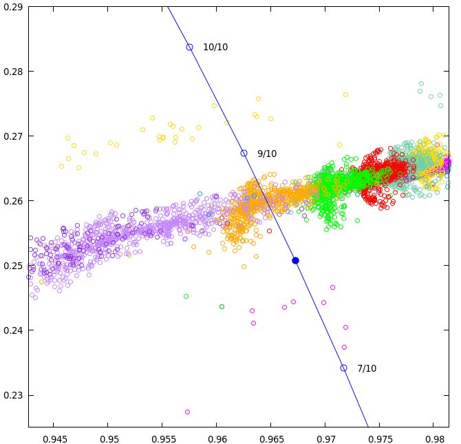
Figure 5: Nodal footprint of the simulated Draconids crossing the ecliptic plane for years of predicted enhanced activity. The
line connects the Earth’s positions at the considered dates.
17The model maximum ZHR profile being about 80 (with a factor 3 uncertainty), we had predicted an activity
not exceeding a few tens of meteors per hour. However, our predictions at the L1 and L2 Lagrange points
suggested storm-level activity at these locations, leading to the temporary re-orientation of the Gaia satellite
(personal communication from Serpell, 2018).
The updated simulated profile for 2018, calibrated using the larger sample of about 22 million particles,
is presented in Figure 4. Compared to our previous work (Egal et al., 2018), we note a slight modification
of the profile shape, but no significant variations of the maximum intensity (90 meteors per hour) or time
(23h45 using the median location method, L = 195.348°). In our simulations, all the particles reaching
Earth belong to the 1953 trail, and have relatively small sizes ([10−3 , 10−2 ] m: 87%, [10−4 , 10−3 ] m: 12%,).
Almost no large particles encountered the Earth.
160
Simulation
IMO/VMBD - rebinned
140 IMO/VMDB
120
100
80
60
40
20
ZHR (met/hr)
0
195.15 195.2 195.25 195.3 195.35 195.4 195.45 195.5 195.55 195.6
120
Simulation
IMO/VMN - rebinned
100 IMO/VMN
80
60
40
20
0
195.15 195.2 195.25 195.3 195.35 195.4 195.45 195.5 195.55 195.6
Solar longitude (o , J2000)
Figure 6: Comparison between the 2018 simulated profile (dark boxes) and preliminary observations released by the Inter-
national Meteor Organization. Visual observations are shown in the top panel & video observations in the bottom panel; the
simulation results are identical in the two panels.
8.2. Observations
At the time of writing, no definitive measurements of the Draconids 2018 have been published. However,
as a preliminary comparison with our predictions, the ZHR profiles issued from the International Meteor
18Organization Visual Meteor Database (IMO/VMDB) and the IMO Video Meteor Network (IMO/VMN)3
were superimposed on the simulation results in Figure 6. The black solid curves represent the original
measurements, and the light boxes the data re-binned in time steps consistent with the simulated profile
(dark boxes). We observe that the length of the simulated profile matches well both sets of observations
and that the peak time estimate is accurate to within a half an hour of uncertainty (depending on when the
maximum activity really occurred). The simulated intensity underestimates the real strength of the shower,
but remains correct within a factor of 2. From these preliminary observations, we conclude that despite the
low number of particles involved in the shower simulation, our model led to one of the best predictions of
the 2018 Draconids published (Egal et al., 2018).
9. Future Draconid outbursts
Finally, in an effort to predict Draconid activity over the next decade, we integrated a sample of particles
generated by Model I until the year 2030. In total, 360 000 particles equally spread over our three size bins
([10−4 , 10−3 ] m, [10−3 , 10−2 ] m and [10−2 , 10−1 ] m) were ejected at each apparition of the comet from 1850
to 2030, resulting in a total of about 9.72 million simulated meteoroids. The model predicted overall peak
intensity of the shower covering the period 2020-2030 is presented in Figure 2.
From this annual variation in the predicted shower strength, we estimate enhanced radio activity in 2019
and 2025, as well as a potential minor display in 2029. Comparing to the predictions of other modelers, we
observe that enhanced activity in 2019 and 2025 is also predicted by Ye et al. (2014) and Maslov (2011).
We however do not share the forecast of a low intensity shower in 2021 mentioned in Ye et al. (2014).
9.1. 2019
On October 8 2019, the model predicted that the Earth will face a similar situation to that in 1999 and
encounter the streams ejected by 21P in 1959 and 1966. Our estimated activity profile, presented in Figure
4, is exclusively composed of particles in the size bin [10−4 , 10−3 ] m. As with the radio outburst in 1999, a
small number of unphysically heavy weighted particles belonging to the 1966 trail raised the ZHR maximum
to a storm value of 5000 meteors per hour and have been removed from the analysis.
The low temporal resolution of the simulated profile, typical of our other simulated radio showers,
decreases the precision of the time and intensity predictions compared to strong visual outbursts. We
estimate, however, that the Earth might experience a radio outburst with a maximum ZHR of about 200
(within a factor of 3), and enhanced activity between 5h45 and 15h30 UT on October 8. The peak time is
difficult to assess from the model profile. If the maximum ZHR is reached around 14h35 UT, (L = 194.753°),
the weighted average of the profile has a peak time of 12h UT (L = 194.648°). When considering the date
of the closest approach between the Earth and the median location of a specific stream, we estimate a
maximum activity caused by the 1959 stream around 13h42 UT (L = 194.718°) and a maximum caused
by the 1966 stream at 12h01 UT. The total duration of the shower, among the longest for radio showers in
our simulations, is 9h45.
Simulations performed by other authors differ from our predictions, either in time and intensity. Results
from the MSFC model, differing from Model I mostly on the ejection circumstances and the weighting
process, augurs for noticeable Draconid activity (nearly as strong as in 2018) culminating around 15h06 UT
on October 8 (L = 194.775°) consisting of mainly smaller particles. A secondary peak might be expected
much earlier, around 4h20 the same day (L = 194.332°). According to Maslov (2011), the activity level
from the 1959 trail in 2019 should be about half of that in 1999. Based on the 1999 ZHR estimated by
(Iiyama in Sato, 2003), Maslov expects “a small visual peak not higher than ZHR 5-10, on 2019 October 8
at 14h45m UT”. He however points out that “radio observations could show much higher activity” (Maslov,
2011).
In Jenniskens (2006), no enhanced Draconid activity was predicted by J. Vaubaillon in 2019. However,
some revised predictions are presented in Table 4. The first one points toward a potential storm on October
3 https://www.imo.net/draconids-outburst-on-oct-8-9/ accessed on 15/12/2018
19You can also read