Methane (CH4) sources in Krakow, Poland: insights from isotope analysis - Recent
←
→
Page content transcription
If your browser does not render page correctly, please read the page content below
Atmos. Chem. Phys., 21, 13167–13185, 2021
https://doi.org/10.5194/acp-21-13167-2021
© Author(s) 2021. This work is distributed under
the Creative Commons Attribution 4.0 License.

Methane (CH4) sources in Krakow, Poland:
insights from isotope analysis
Malika Menoud1 , Carina van der Veen1 , Jaroslaw Necki2 , Jakub Bartyzel2 , Barbara Szénási3 , Mila Stanisavljević2 ,
Isabelle Pison3 , Philippe Bousquet3 , and Thomas Röckmann1
1 Institute
          for Marine and Atmospheric research Utrecht (IMAU), Utrecht University, Utrecht, the Netherlands
2 Facultyof Physics and Applied Computer Science, AGH University of Science and Technology, Krakow, Poland
3 Laboratoire des sciences du climat et de l’environnement (LSCE), Université Paris-Saclay,

CEA, CNRS, UVSQ, Gif-sur-Yvette, France

Correspondence: Malika Menoud (m.menoud@uu.nl)

Received: 18 February 2021 – Discussion started: 22 April 2021
Revised: 13 July 2021 – Accepted: 2 August 2021 – Published: 6 September 2021

Abstract. Methane (CH4 ) emissions from human activities            The CHIMERE transport model was used to compute
are a threat to the resilience of our current climate system.    the CH4 and isotopic composition time series in Krakow,
The stable isotopic composition of methane (δ 13 C and δ 2 H)    based on two emission inventories. The magnitude of the
allows us to distinguish between the different CH4 origins.      pollution events is generally underestimated in the model,
A significant part of the European CH4 emissions, 3.6 % in       which suggests that emission rates in the inventories are
2018, comes from coal extraction in Poland, the Upper Sile-      too low. The simulated isotopic source signatures, obtained
sian Coal Basin (USCB) being the main hotspot.                   with Keeling plots on each simulated peak, indicate that
Measurements of CH4 mole fraction (χ(CH4 )), δ 13 C, and         a higher contribution from fuel combustion sources in the
δ 2 H in CH4 in ambient air were performed continuously dur-     EDGAR v5.0 inventory would lead to a better agreement
ing 6 months in 2018 and 2019 at Krakow, Poland, in the east     than when using CAMS-REG-GHG v4.2 (Copernicus Atmo-
of the USCB. In addition, air samples were collected during      sphere Monitoring Service REGional inventory for Air Pol-
parallel mobile campaigns, from multiple CH4 sources in the      lutants and GreenHouse Gases). The isotopic mismatches be-
footprint area of the continuous measurements. The resulting     tween model and observations are mainly caused by uncer-
isotopic signatures from sampled plumes allowed us to dis-       tainties in the assigned isotopic signatures for each source
tinguish between natural gas leaks, coal mine fugitive emis-     category and the way they are classified in the inventory.
sions, landfill and sewage, and ruminants. The use of δ 2 H in   These uncertainties are larger for emissions close to the study
CH4 is crucial to distinguish the fossil fuel emissions in the   site, which are more heterogenous than the ones advected
case of Krakow because their relatively depleted δ 13 C val-     from the USCB coal mines. Our isotope approach proves to
ues overlap with the ones of microbial sources. The observed     be very sensitive in this region, thus helping to evaluate emis-
χ(CH4 ) time series showed regular daily night-time accumu-      sion estimates.
lations, sometimes combined with irregular pollution events
during the day. The isotopic signatures of each peak were
obtained using the Keeling plot method and generally fall
in the range of thermogenic CH4 formation – with δ 13 C be-      1   Introduction
tween −59.3 ‰ and −37.4 ‰ Vienna Pee Dee Belemnite (V-
PDB) and δ 2 H between −291 ‰ and −137 ‰ Vienna Stan-            Atmospheric emissions of greenhouse gases, defined as gas
dard Mean Ocean Water (V-SMOW). They compare well                compounds that absorb and emit thermal infrared radiations
with the signatures measured for gas leaks in Krakow and         from human activities are the main cause of the current
USCB mines.                                                      warming of our Earth’s climate. It is urgent to decrease these
                                                                 emissions in order to minimise the negative consequences

Published by Copernicus Publications on behalf of the European Geosciences Union.
13168                                                              M. Menoud et al.: Methane (CH4 ) sources in Krakow, Poland

of climate change on people and societies (IPCC, 2018).                where most mining activity occurs in Poland, is certainly
The second most important greenhouse gas of anthropogenic              a CH4 emission hotspot in Europe. Atmospheric measure-
origin after carbon dioxide (CO2 ) is methane (CH4 ; IPCC,             ments at the USCB have mostly been performed in recent
2018). CH4 has a global warming potential (GWP; integrated             years (Swolkień, 2020; Luther et al., 2019; Gałkowski et al.,
radiative forcing relative to that of CO2 per kilogram of emis-        2020; Fiehn et al., 2020) and focused on the coal extraction
sion) of 86 over a 20-year time horizon, including carbon              activities. The CH4 emission rates were estimated at the re-
cycle feedbacks (IPCC, 2013). On a global scale, 23 % of               gional scale (Luther et al., 2019; Fiehn et al., 2020), with a
the additional radiative forcing since 1750 is attributed to           relatively good agreement with the inventories (Luther et al.,
CH4 , whereas total CH4 anthropogenic emissions represent              2019; Fiehn et al., 2020; Gałkowski et al., 2020). Swolkień
only 3 % of those of CO2 in term of carbon mass flux (Et-              (2020) performed direct measurements of CH4 fluxes at in-
minan et al., 2016). In recent years, total CH4 emissions              dividual shafts and emphasised the large variability of emis-
have been rising: they increased by 5 % in the period 2008–            sion patterns between different sites. A general isotopic sig-
2017 (and 9 % in 2017), compared to the period 2000–2006               nature from USCB CH4 sources was recently determined
(Saunois et al., 2020). It is not clear which sources caused           by Gałkowski et al. (2020), with values of −50.9 ± 1.1 ‰
these changes, but Saunois et al. (2020) estimated anthro-             for δ 13 C and −224.7 ± 6.6 ‰ for δ 2 H. These values, based
pogenic emissions to represent 60 % of the total emissions of          on aircraft measurements, compare well with previous mea-
the past 10 years. Nisbet et al. (2019) showed that the cur-           surements at individual shafts for δ 13 C but are significantly
rent levels of CH4 emissions are a threat to the adherence of          lower for δ 2 H. The area covered by the USCB includes other
the Paris Agreement goals, but an effective reduction of CH4           sources of methane, such as ruminant farming and waste
emissions requires knowledge of the locations and magni-               degradation. In this study we investigate whether we can use
tudes of the different sources.                                        isotopic signals to distinguish the different sources from a
   Atmospheric measurements of greenhouse gases at sev-                densely populated area like Krakow. We wanted to establish
eral locations have been used to investigate the rates, origins,       the main CH4 sources affecting the city. Finally, we investi-
and variations in emissions. However, for methane, these are           gate whether we can use this tool to put constraints on the
not always in agreement with what is reported in the emis-             emission inventories in order to improve them.
sions inventories (Saunois et al., 2020). Isotopic measure-               To this end, we carried out and investigated quasi-
ments are used to better constrain the sources of methane at           continuous measurement of the CH4 mole fraction and
regional (e.g. Levin et al., 1993; Tarasova et al., 2006; Beck         13 C/12 C and 2 H/1 H isotopic ratios of CH in ambient air
                                                                                                                     4
et al., 2012; Röckmann et al., 2016; Townsend-Small et al.,            during 6 months at a fixed location in Krakow, Poland. Time
2016; Hoheisel et al., 2019; Menoud et al., 2020b) and global          series of these isotopic ratios were also simulated with an at-
scales (e.g. Monteil et al., 2011; Rigby et al., 2012; Schwi-          mospheric transport model, based on two different emission
etzke et al., 2016; Schaefer et al., 2016; Nisbet et al., 2016;        inventories. The local CH4 sources were sampled during sev-
Worden et al., 2017; Turner et al., 2019). Indeed, the differ-         eral mobile measurement campaigns to determine their iso-
ent CH4 generation pathways lead to different isotopic signa-          topic signatures and compare these with the ambient mea-
tures (Milkov and Etiope, 2018; Sherwood et al., 2017; Quay            surements.
et al., 1999). Recently, instruments for continuous measure-
ments of the isotopic composition of CH4 have been devel-
oped (Eyer et al., 2016; Chen et al., 2016; Röckmann et al.,           2     Methods
2016) and used to characterise the main sources of a spe-
cific region (Röckmann et al., 2016; Yacovitch et al., 2020;           2.1    Target region and time period
Menoud et al., 2020b). Using model simulations, the obser-
vations can be used to evaluate the partitioning of the differ-        The region of study is characterised by the presence of a large
ent sources reported in the inventories (Rigby et al., 2012;           coal mining region: the Upper Silesian Coal Basin (USCB).
Szénási, 2020).                                                        It has 20 active coal mines spread over an area of 1100 km2
   Saunois et al. (2020) stated the need for more measure-             (Swolkień, 2020), and the closest shafts are located about
ments in regions where very few observations have been                 40 km west of Krakow (Fig. 1). Other potential CH4 sources
available so far. In Europe, inventories report high CH4 emis-         around Krakow are from waste management and wastewa-
sions from Poland (European Environment Agency, 2019).                 ter treatment facilities, industrial activity, energy production,
In 2018, they represented 10 % of total European Union                 and the natural gas distribution network. Large-scale agricul-
(EU) emissions, with more than 48 Mt CO2 eq. Half of these             ture activities are not characteristic of this area, and only very
are from the energy sector, among which 72 % are due to                few cattle farms could be located.
the exploitation of underground coal mines (National Cen-                 Ambient air measurements were performed from the Fac-
tre for Emission Management (KOBiZe) and Institute of En-              ulty of Physics and Applied Computer Science building, at
vironmental Protection – National Research Institute 2020;             AGH university in Krakow (50◦ 040 01.100 N, 19◦ 540 46.900 E;
Swolkień, 2020). The Upper Silesian Coal Basin (USCB),                Fig. 1). We used a 1/2 in. o.d. Synflex Dekabon air intake

Atmos. Chem. Phys., 21, 13167–13185, 2021                                               https://doi.org/10.5194/acp-21-13167-2021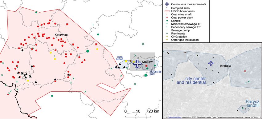
M. Menoud et al.: Methane (CH4 ) sources in Krakow, Poland                                                                            13169

Figure 1. Location of the long-time measurements, sampled sites, and potential anthropogenic methane sources. Note that this is not an
exhaustive list: not all the sewage pumps are reported, and no official information on cattle farms was obtained. Other emissions from mining
activities, coming from processing facilities or waste disposal, are not reported here. No χ(CH4 ) enhancements were measured around
stagnant water bodies, therefore they are not all reported here (TP denotes the treatment plant, and CNG denotes the compressed natural gas).
© OpenStreetMap contributors 2021. Distributed under the Open Data Commons Open Database License (ODbL) v1.0.

line that draws air from the top of a mast on top of the                 If the increase was higher than 200 ppb above background,
building (35 m a.g.l., 255 m a.s.l.) down to the laboratory of           we drove back to the plume and took one to three samples
the Environmental Physics Group. A fraction of the incom-                directly from the outflow of the CH4 analyser, using sam-
ing air was directed via a T-split to the isotope ratio mass             pling bags (Supel™-Inert Multi-Layer Foil, Sigma-Aldrich
spectrometry (IRMS) system in the period from 14 Septem-                 Co. LLC).
ber 2018 to 14 March 2019. To put the CH4 enhance-                          One or two samples were taken where we observed the
ments in perspective, the data were compared with measure-               lowest χ(CH4 ) during each survey day, in order to obtain the
ments of background CH4 made by the KASLAB (high-                        background we can associate with the plumes sampled each
altitude laboratory of greenhouse gas measurement) at the                day in a certain area.
top of at Kasprowy Wierch, a mountain in southern Poland                    The samples collected during the mobile surveys were
(49◦ 130 5700 N, 19◦ 580 5500 E; 1989 m a.s.l.; Necki et al., 2013).     analysed on the same IRMS instrument as the ambient air,
   Individual emission locations of methane were visited in              partly when it was installed in Krakow and partly when it
and around the city of Krakow and in the USCB during mo-                 was installed back at the IMAU lab in Utrecht.
bile surveys. The surveys were performed in May 2018 (from
24th to 29th), February 2019 (from 5th to 7th), and March                2.3   Isotopic measurements
2019 (from 20th to 22th). We visited the following areas,
which are shown on the map in Fig. 1: the Silesian Coal                  The 13 C/12 C and 2 H/1 H isotope ratios in CH4 are expressed
Basin, Barycz landfill, the industrial park, the city centre and         as δ 13 C and δ 2 H (deuterium), respectively, in per mil (‰),
other residential areas, and rural areas west of the city.               relative to the international reference materials, Vienna Pee
                                                                         Dee Belemnite (V-PDB) for δ 13 C and Vienna Standard Mean
2.2   Sampling                                                           Ocean Water (V-SMOW) for δ 2 H.
                                                                            The isotopic composition measurements were performed
The mobile surveys were conducted with an integrated cavity              using an isotope ratio mass spectrometry (IRMS) sys-
output spectroscopy (ICOS) instrument (MGGA – 918, Mi-                   tem, as described in Röckmann et al. (2016) and Menoud
croportable Greenhouse Gas Analyser, Los Gatos Research,                 et al. (2020b). Ambient air or sample air measure-
ABB) onboard a car. An 1/8 in. Parflex inlet line was placed             ments were interspersed with measurements of a refer-
on top of the vehicle’s roof and connected to the analyser.              ence cylinder filled with air with assigned composition
Real-time CH4 mole fractions were read on a tablet screen,               of χ (CH4 ) = 1950.3 ppb, δ 13 C–CH4 = −47.82 ± 0.09 ‰ V-
so that an emission plume could be detected while driving.               PDB, and δ 2 H–CH4 = −92.2 ± 1.8 ‰ V-SMOW. The refer-

https://doi.org/10.5194/acp-21-13167-2021                                               Atmos. Chem. Phys., 21, 13167–13185, 2021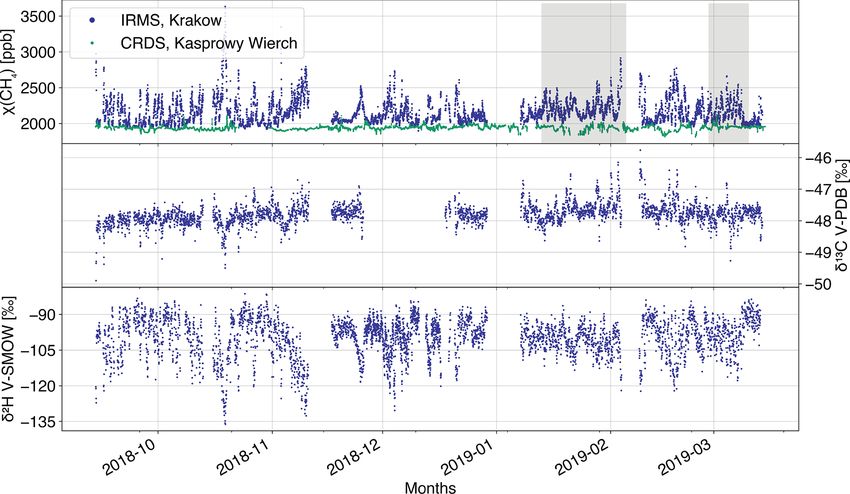
13170                                                               M. Menoud et al.: Methane (CH4 ) sources in Krakow, Poland

ence air bottle was previously calibrated against a reference           Weather Forecast (ECMWF) operational forecast product.
gas measured at the Max Planck Institute in Jena, Germany               The boundary and initial concentrations of χ(CH4 ) were
(Sperlich et al., 2016).                                                taken from the analysis and forecasting system developed
    The extraction and measurement steps are illustrated in             in the Monitoring Atmospheric Composition and Climate
Fig. S1 in the Supplement. Each measurement of either δ 13 C            (MACC) project (Marécal, 2015). They were used to derive
or δ 2 H returned a value of CH4 mole fraction (χ(CH4 )), cal-          the background CH4 mole fractions.
culated from the area of the IRMS peak obtained for the                    The CH4 emission rates over the domain are reported in
sample, compared to the area of air from a reference gas                emission inventories, following a bottom-up approach. We
cylinder filled with air with 1950.3 ppb CH4 . This cylinder            used two anthropogenic emission inventories for this study:
was calibrated against a reference gas measured by the Max              EDGAR v5.0 (Emission Database for Global Atmospheric
Planck Institute for Biogeochemistry, Jena, Germany. The                Research; Crippa et al., 2019) and CAMS-REG-GHG v4.2
reproducibility of our measurements is 16 ppb for χ(CH4 ),              (Copernicus Atmosphere Monitoring Service REGional in-
0.07 ‰ for δ 13 C and 1.7 ‰ for δ 2 H. A δ 13 C–CH4 or δ 2 H–           ventory for Air Pollutants and GreenHouse Gases; Granier
CH4 value in ambient air was obtained on average every                  et al., 2012). We classified the emissions in six anthro-
27 min during the periods of normal operation. In addition to           pogenic source categories based on the European Environ-
unexpected disturbances or failures, the scheduled replace-             ment Agency (EEA) greenhouse gas inventory common re-
ment of several components (oven catalysts, chemical dryer,             porting format (CRF, European Environment Agency, 2019).
fittings, etc.) and the regular flushing and heating of the traps       We considered one additional category for natural wetland
required to stop the measurements for a few hours up to a               emissions, which are obtained from the ORCHIDEE-WET
few days, several times during the study period.                        process model (Ringeval et al., 2011). The classifications
    The air was simultaneously measured by a cavity ring-               used in CHIMERE and the corresponding categories in the
down spectroscopy (CRDS) instrument (G2201-i isotopic                   inventories are summarised in Table 1.
analyser, Picarro) installed in the same lab as the IRMS sys-              The isotopic values at each time t were calculated using
tem and drawing air from the same inlet tube. Time series of            the following formula:
CH4 mole fractions from both instruments were compared
                                                                                  nS
for quality control, but we did not evaluate the isotopic ratios               1X
                                                                        δt =         (cS,i · δS,i ),
from the CRDS. The instrument precision for the CH4 mole                       ct i
fraction is of 6 ppb, as reported by the manufacturer.
                                                                        with ct the total mole fraction from the model at time t, cS
2.4   Meteorological data                                               the modelled mole fraction attributed to the source S, and δS
                                                                        the source signature of each specific source S. In this mass
Data on the hourly wind direction, speed, and temperature               balance, the contribution of the background is treated as a
were obtained from an automatic weather station (Vaisala                source with assigned isotopic composition. All the assigned
WXT520, Vaisala Inc.) installed on the same building as the             source signatures are defined in Table 1.
inlet line (220 m a.s.l.). The station is operated by the En-
vironmental Physics Group, and the data are publicly avail-             2.6    Isotopic signatures assigned to CH4 enhancements
able at http://meteo.ftj.agh.edu.pl/archivalCharts (last access:
21 October 2020) (registration required). Data on PM10 con-             Periods of methane enhancement were identified from the
centrations are also available on the same platform at this             χ(CH4 ) time series using a peak extraction method, based
location.                                                               on the detection of local maxima from comparison with the
                                                                        neighbouring points. The peaks were selected based on two
2.5   Modelling                                                         criteria:

                                                                          – The peak has a minimal amplitude of 100 ppb.
Time series of δ 13 C–CH4 and δ 2 H–CH4 were generated from
simulated CH4 mole fractions using the CHIMERE atmo-                      – The peak is composed of at least three data points, from
spheric transport model (Menut et al., 2013; Mailler et al.,                the maximum to a relative height of 0.6 times the peak
2017), driven by the PYVAR system (Fortems-Cheiney et al.,                  height.
2019). CHIMERE is a three-dimensional Eulerian limited-
area chemistry-transport model for the simulation of regional           In order to define the background more robustly, we included
atmospheric concentrations of gas-phase and aerosol species.            additional data from the 10th lower percentile of χ(CH4 ) in
   The simulations were carried out at a horizontal resolu-             a window of ±24 h around the maximum of each peak. The
tion of 0.1◦ × 0.1◦ in a domain covering Poland and nearby              Keeling plot method was thus applied to the data points in
countries, [46.0–55.9◦ ] in latitude and [12.0–25.9◦ ] in lon-          the peak, together with the neighbouring background data.
gitude. The meteorological data used to drive CHIMERE                      The Keeling plot is a mass balance approach (Keeling,
were obtained from the European Centre for Medium-Range                 1961; Pataki et al., 2003), considering the measured CH4 (m)

Atmos. Chem. Phys., 21, 13167–13185, 2021                                                  https://doi.org/10.5194/acp-21-13167-2021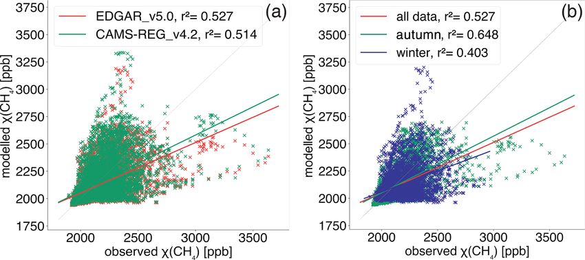
M. Menoud et al.: Methane (CH4 ) sources in Krakow, Poland                                                                                                         13171

Table 1. Methane emission categories considered for this study, with the corresponding classification in the inventories, and the respective
isotopic signature used to compute δ 13 C and δ 2 H time series with CHIMERE. If no references are specified, the assigned isotope values are
derived from the sampling campaigns we carried out in the study area and described in this paper.

  CHIMERE           CRF sectora                             IPCC 2006         EDGAR v5.0                CAMS-REG-GHG v4.2 sector        Assigned δ 13 C   Assigned δ 2 H
  source category                                           code              sector                                                    V-PDB [‰]         V-SMOW [‰]
  Agriculture       3                Agriculture            3A1               Enteric fermentation      K             Agriculture       −61.5             −356
                                                                                                                      – livestock
                                                            3A2               Manure management
                                                            3C1b              Agriculture waste         L             Agriculture
                                                                              burning                                 – other
                                                            3C2, 3C3, 3C4,    Agriculture soils
                                                            3C7
  Waste             5                Waste                  4A, 4B            Solid waste landfills     J             Waste             −51.3             −308
                                                            4C                Solid waste
                                                                              incineration
                                                            4D                Waste water handling
  Fossil fuels      1B               Energy – fugitive      1B1a              Fuel exploitation, coal   D             Fugitives         −50.7             −190
                                     emissions from
                                     fuels
                                                            1bB2bi, 1B2bii    Fuel exploitation, gas                                    −49.3             −195
                                                            1B2aiii2,         Fuel exploitation, oil                                    −49.8             −193
                                                            1B2aiii3
  Non-industrial    1A4,             Energy – other         1A4, 1A5          Energy for buildings      C             Other             −32.1c            −185c
  combustion        1A5              sectors, otherb                                                                  stationary
                                                                                                                      combustion
  Other             1A               Energy – industries    1A1a              Power industry            A             Public power      −49.8             −193
  anthropogenic
                                                            1A1b, 1A1ci,      Oil refineries and
                                                            1A1cii,           transformation industry
                                                            1A5biii,
                                                            1B1b, 1B2aiii6,
                                                            1B2biii3, 1B1c
                    2                Industrial processes   1A2               Combustion for            B             Industry
                                     and product use                          manufacturing
                                                            5B                Fossil fuel fires
                                                            2B                Chemical processes
                                                            2C1, 2C2          Iron and steel
                                                                              production
                                                            2D3, 2E, 2F,      Solvents and products     E             Solvents
                                                            2G                use
                    1A3              Energy – transport     1A3b              Road transportation       F             Road transport
                                                            1A3d              Shipping                  G             Shipping
                                                            1A3a              Aviation                  H             Aviation
                                                            1A3c, 1A3e        Railways, pipelines,      I             Off-road
                                                                              off-road transport
  Wetlands                                                                                                                              −73.2c            −323c
  Background                                                                                                                            −47.8             −89

a European Environment Agency (2019). b Mostly the use of coal for heating households (European Environment Agency, 2019). c Menoud et al. (2020a, b).

in ambient air as the sum of a contribution of CH4 from an                                   We assumed the background mole fraction and isotopic com-
emission source (s) and a background (bg) CH4 , such that                                    position to be stable over the time period of each peak. In
                                                                                             this case, δs is given by the y intercept of the regression line,
cm = cbg + cs                                                                                when plotting δm against 1/cm .
                                                                                                To derive an average source signature for the entire
cm δm = cbg δbg + cs δs ,                                                                    dataset, the Miller–Tans approach was used (Miller and Tans,
with c and δ referring to the mole fraction and isotopic signa-                              2003) because the hypothesis of stable background is vio-
tures of either 13 C or 2 H, respectively. Rearranging the for-                              lated. This method is based on the following formula:
mula leads to

δm = cbg · (δbg − δs )(1/cm ) + δs .                                                         cm δm = δs cm − cbg (δbg − δs ),

https://doi.org/10.5194/acp-21-13167-2021                                                                    Atmos. Chem. Phys., 21, 13167–13185, 2021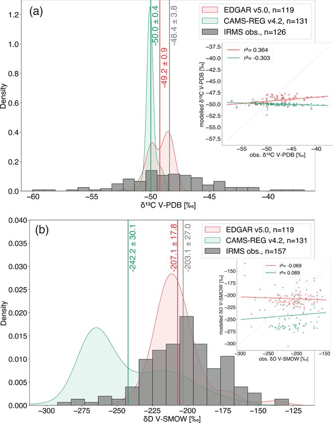
13172                                                              M. Menoud et al.: Methane (CH4 ) sources in Krakow, Poland

Figure 2. Time series of the observed χ (CH4 ) (n = 7886), δ 13 C (n = 3477), and δ 2 H (n = 4389), together with the χ (CH4 ) time series
observed at Kasprowy Wierch (green; n = 21 028). The shaded areas show when there was a mismatch between the IRMS and CRDS
instruments in the mole fractions.

where δs is now given by the slope of the regression line,             3     Results and discussion
when plotting cm · δm against cm .
    An isotopic signature was obtained from the linear regres-         3.1    Observed time series
sions, and the corresponding uncertainty was derived as 1
standard deviation of the estimated parameter (intercept for           The observed time series are shown in Fig. 2, together with
the Keeling plot or slope for the Miller–Tans plot). For all           measurements of CH4 at Kasprowy Wierch. We note that in
Keeling plots, the weighted orthogonal distance regression             the period February–March 2019, we observed a mismatch
(ODR) fitting method (Boggs et al., 1992) was used.                    of about 80 ppb between the IRMS-derived and simultane-
    The method was applied to both δ 13 C and δ 2 H measure-           ous CRDS χ(CH4 ) measurements in the same laboratory
ment results. If two peaks were detected within a 6 h time             (shaded area in Fig. 2). A mismatch in mole fraction can
window in the δ 13 C and δ 2 H time series, they were consid-          potentially affect the Keeling plot intercepts, and we investi-
ered one single peak and the two signatures were allocated to          gated possible artefacts using various attempts for correction.
it. The same method was also used for the modelled χ(CH4 )             We realised that the effect of these corrections on the isotopic
time series, to allow for the comparison of modelled and               source signatures is small compared to the observed range
measured source signatures.                                            (average peak δ 13 C and δ 2 H changed by 0.1 %; different peak
    The Keeling plot method was also used to calculate source          source signatures are shown in Fig. S5b). As no obvious rea-
isotopic signatures for each location where we sampled CH4             son for a malfunction of the IRMS instrument could be de-
enhancements during the mobile surveys. The determined                 tected, we decided to use the original data without correction.
source signatures were accepted if they fulfilled at least two         The peaks in χ(CH4 ), compared to the background measured
of the following criteria for both δ 13 C and δ 2 H: (i) χ(CH4 )       at Kasprowy Wierch, reflect pollution events in Krakow or
above background > 90 ppb, (ii) Pearson’s coefficient r 2 of           advected to the measurement site. The maximum χ(CH4 )
the linear fit > 0.75, and (iii) the standard deviation of the         value was 3634 ppb, measured on 19 October 2018 at 05:30.
y intercept lower than 5 ‰ for δ 13 C and 100 ‰ for δ 2 H re-          Simultaneous changes are visible in the δ 13 C and δ 2 H time
spectively.                                                            series. Increased χ(CH4 ) values were always linked with a
                                                                       lower δ 2 H, but for δ 13 C the measured values could be higher
                                                                       or lower.

Atmos. Chem. Phys., 21, 13167–13185, 2021                                                https://doi.org/10.5194/acp-21-13167-2021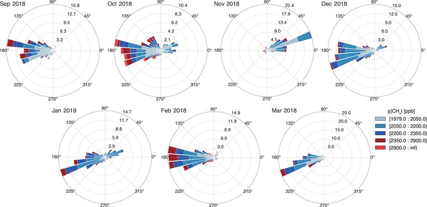
M. Menoud et al.: Methane (CH4 ) sources in Krakow, Poland                                                                        13173

Figure 3. Monthly wind directions during the ambient air measurement period, at the same location. Bar lengths are percentages of records
during the specified month (r axis); colours define the χ (CH4 ) range (legend).

   The general background threshold is 1986.0 ppb, which               the east/north-east direction. March 2019 was characterised
corresponds to the 10th lower percentile of the entire                 by winds from the west only and at particularly strong speeds
dataset. We have found that 70.5 % of the background values            (on average 3.1 m s−1 , compared to 1.8 m s−1 for the other
(χ(CH4 ) < 1986.0 ppb) occurred during daytime. The domi-              months; Fig. S3). The average CH4 diurnal cycle, defined
nant feature in the CH4 time series is indeed the presence of a        as the prominence of night peaks, was on average 334 ppb
diurnal cycle: χ(CH4 ) enhancements regularly occurred dur-            throughout the entire time period but only 195 ppb when the
ing the night. This is due to a lowering of the boundary layer         winds were > 2.5 m s−1 . This decrease in amplitude with
when the temperature gradient decreases in the evening. The            higher wind speeds was not influenced by the direction of
morning and evening variations in χ(CH4 ) were negatively              the wind. During fall, 84 % of the peaks were observed at
correlated with the temperature data we obtained at the study          night and associated with low wind speeds, which suggests
site. In addition, there were isolated pollution events occur-         the influence of local pollution sources and a relatively low
ring on top of the night-time accumulation. Between peaks,             influence of the wind direction.
χ(CH4 ) generally went back to a local background level.                   The average isotopic values of the background were
   The night-time accumulation was particularly visible in             δ 13 C = −47.8 ± 0.1 ‰ and δ 2 H = −89 ± 3 ‰. The CH4 en-
the period 14 September to mid-November 2018 and is                    hancements were associated with consistently more negative
shown in the Supplement (Fig. S2). Similar night-time en-              δ 2 H but varying δ 13 C. This indicates that the sources were
hancements are also visible in the observations of other pol-          sometimes higher in δ 13 C compared to the ambient CH4 (i.e.
lutants such as PM10 at the study location. There was a clear          δ 13 C > −47.8 ‰). In contrast, all CH4 enhancements were
difference in local temperature before and after 15 November           associated with lower δ 2 H during the entire time period.
2018: the average air temperature decreased from 12 ± 5.3 to
2.1 ± 4.4 ◦ C and the dew point temperature from 5.3 ± 3.4 to          3.2   Modelled time series
−3.9 ± 3.4 ◦ C until the end of the measurements. The period
before mid-November will be referred to as autumn through-             The CH4 time series obtained with CHIMERE for the grid
out the paper.                                                         cell containing the observation site are shown in Fig. 4. We
   The wind directions at the study site were combined with            first compared the CH4 mole fractions measured at Krakow
the CH4 measurement data in Fig. 3 and with wind speeds                and modelled by CHIMERE in Fig. 5. They show a poor
in Fig. S3. The spread of the wind directions was similar              correlation (Pearson’s correlation coefficients r 2 = 0.527
for most of the months: mainly from the west (70 %), with a            and r 2 = 0.514, for model calculations using the EDGAR
small contribution (27 %) from the east/north-east. An excep-          v5.0 and CAMS-REG-GHG v4.2 inventories, respectively;
tion was November 2018, when most of the wind was from                 Fig. 5a). The model globally underestimates the measured

https://doi.org/10.5194/acp-21-13167-2021                                             Atmos. Chem. Phys., 21, 13167–13185, 2021
13174                                                           M. Menoud et al.: Methane (CH4 ) sources in Krakow, Poland

Figure 4. Time series of the observed (blue circles) and modelled χ (CH4 ), δ 13 C and δ 2 H, based on the EDGAR v5.0 (red) and CAMS-
REG-GHG v4.2 (green) inventories.

Figure 5. Correlation between observed and modelled χ (CH4 ) values, using (a) the EDGAR v5.0 (red) or the CAMS-REG-GHG v4.2
(green) inventories and (b) different time periods: autumn (14 September to 15 November 2018; green) or winter (15 November 2018 to
15 March 2019; blue) computed using EDGAR v5.0.

χ(CH4 ) significantly, with a root mean square error (RMSE)          2018, using EDGAR v5.0 (r 2 = 0.648; Fig. 5b). As men-
of 164.4 and 173.4 ppb for EDGAR and CAMS, respec-                   tioned in Sect. 3.1, autumn 2018 shows a more regular pat-
tively. Yet we see that modelled χ(CH4 ) can sometimes be            tern of night-time enhancements of relatively similar am-
larger than the observations, which is usually due to a shift        plitudes compared to the winter period. This is better re-
in the timing of a pollution event (Fig. 4). The wind data           produced by the model (Fig. 4). However, the two highest
used in the model are generally in good agreement with the           χ (CH4 ) measurements were observed in this period (18 Oc-
wind measurements at the study site, but small discrepan-            tober, and 3 November 2018) and were not modelled to the
cies can partly explain the differences in the timing of the         same level (points on the lower right, Fig. 5b). These events
peaks. The time series are best reproduced during autumn

Atmos. Chem. Phys., 21, 13167–13185, 2021                                            https://doi.org/10.5194/acp-21-13167-2021
M. Menoud et al.: Methane (CH4 ) sources in Krakow, Poland                                                                  13175

largely contribute to the general model underestimation when       The derived isotopic signatures are in good agreement with
only considering the autumn data.                                  the ranges defined for the different categories in the litera-
   In winter, the χ(CH4 ) enhancements were less regular,          ture (Sherwood et al., 2017). Biogenic sources (a landfill,
with a less consistent diurnal cycle (Fig. S2). The mismatch       three manholes, and a cow barn) correspond to the acetate
in the timing of pollution events caused an overestimation         fermentation pathway, characterised by relatively depleted
by the model (points on the upper left, Fig. 5b). The gen-         δ 13 C (< −50 ‰) and δ 2 H (< −275 ‰; Milkov and Etiope,
eral slope is still lower than 1, and the fit is worse than dur-   2018). The landfill CH4 is isotopically more enriched than
ing fall. There is a general underestimation of the CH4 mole       the cow barn. This can be due to an isotope fractionation
fractions at Krakow by the model. This could be explained          from diffusion and oxidation in the soil layers (De Visscher,
by the model time series being hourly averages, compared           2004; Bakkaloglu et al., 2021). The fossil fuel CH4 emissions
to the observations of sampled air. To account for this bias,      we sampled were from coal exploitation and use of natural
we compared the model data with observations that are also         gas. The natural gas distribution network was sampled out-
averaged over a 1 h window and/or interpolated to the mod-         side of compressor stations, close to gas stations and sup-
elled times. This had no effect on the correlation coefficients,   ply valves in residential areas. The results ranged between
suggesting a minor impact of the temporal representation er-       [−52.3, −44.4] ‰ for δ 13 C and [−225, −177] ‰ for δ 2 H.
ror. Another reason for the underestimation of χ(CH4 ) in          To check for temporal variations, four plumes were sampled
CHIMERE could be the presence of potential CH4 sources             at an interval of 6 weeks, on 5 February and 19 March 2019.
in the close surroundings of the laboratory. Such emissions        The δ 13 C results were about 4.7 ‰ more depleted, and the
could affect the measurements but not the model, where they        δ 2 H results were 27 ‰ more depleted in March compared to
are diluted over the 11 km grid cell. The misfit between mod-      February. One sample was directly taken from the gas sup-
elled and observed χ(CH4 ) could also be due to some errors        ply pipe at the AGH lab in March 2019. The pure gas was
in the transport modelling or insufficient emissions in the in-    3.6 ‰ and 14 ‰ more depleted in δ 13 C and δ 2 H, respec-
ventories. Szénási (2020) identified the emission inventories      tively, than the average from accidental leaks (signature in
as the main source of discrepancies between CHIMERE re-            brackets in Table 2), which indicates that the isotopic com-
sults and measured time series at two other European loca-         position of the city gas in March is relatively depleted com-
tions. The implications on the two inventories are discussed       pared to February. The network gas composition can change
in detail in Sect. 3.4.                                            in time because the proportions of gas from several origins
   Time series of δ 13 C and δ 2 H in CH4 show negative or pos-    vary. Gas migrating in the distribution network can undergo
itive excursions relative to the background and are linked to      secondary processes. For example CH4 oxidation into CO2
χ(CH4 ) peaks (Fig. 4). When using CAMS-REG-GHG v4.2,              influences the isotopic signatures, usually towards more en-
δ 13 C and δ 2 H are always negatively correlated with χ(CH4 ).    riched values. Isotopic variations among network gas leaks
But when using the EDGAR v5.0 inventory, δ 13 C values are         were also observed previously in other cities (Zazzeri et al.,
closer to the background. The isotopic discrepancies will be       2017; Maazallahi et al., 2020; Defratyka et al., 2021). The
analysed in detail in relation to the source partitioning in the   isotopic signature of the pure gas we sampled still falls in the
inventories and the signatures we assigned to each source in       same range as the sampled leaks.
Sect. 3.4.                                                             CH4 emissions from manholes were often observed in the
                                                                   Krakow urban area. The resulting isotopic signatures do not
3.3     Isotopic source signatures                                 indicate one clear origin and were divided in two groups
                                                                   with distinct δ 2 H (Table 2). While the isotopically depleted
A total of 126 and 157 peaks were identified in the δ 13 C and     signatures observed at three locations likely come from the
δ 2 H time series, respectively, and 114 peaks were measured       sewage system, with a δ 2 H < −300 ‰, the five others con-
commonly by both isotope lines. From the Keeling plot ap-          tain CH4 with particularly enriched δ 2 H (between −202 ‰
plied to each of the peaks, we obtained the source signatures      and −146 ‰), not typical of microbial fermentation pro-
of the corresponding accumulation events. They can be com-         cesses (Fig. S5a). We hypothesise that this indicates leakage
pared with the determined isotope signatures of the sources        of natural gas from the distribution pipes to the sewage net-
sampled in the surrounding area (Fig. 6a).                         work, which is sometimes further oxidised, leading to even
                                                                   more enriched isotope signatures.
3.3.1    Isotopic characterisation of the surrounding                  For most emission plumes, we could not visually identify
         sources during mobile surveys                             an obvious CH4 source. The isotopic signatures of these “un-
                                                                   known” sources range from −58.2 ‰ to −34.9 ‰ V-PDB
The results from 55 individual sites are presented in Table 2      for δ 13 C and from −285 ‰ to −142 ‰ V-SMOW for δ 2 H.
and shown in detail in the Supplement (Table S1 in the Sup-        These large ranges in δ 13 C and δ 2 H indicated the presence
plement and Fig. S5a). The maximal χ(CH4 ) sampled at each         of both fossil fuel and biogenic sources. The average δ 2 H
location varied between 93 ppb above background and 95 %           is > 200 ‰, suggesting a major influence from fossil fuel
(pure gas), with a median of 1480 ppb above background.            sources. The δ 13 C is in good agreement with the signature

https://doi.org/10.5194/acp-21-13167-2021                                        Atmos. Chem. Phys., 21, 13167–13185, 2021
13176 M. Menoud et al.: Methane (CH4 ) sources in Krakow, Poland
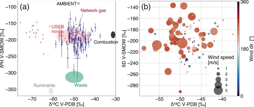
Figure 6. Dual isotope plots of the resulting source signatures from the CH4 peaks identified in the time series. (a) Dark blue: source
signatures with their associated 1σ uncertainties. Coloured areas: ranges of source signatures obtained from the collected samples. If based
on one location (ruminants and combustion), the size of the ellipse is 1 order of magnitude of the precision of our isotopic measurements. Red
dots: source signatures of USCB coal gas derived from Kotarba (2001), Kotarba and Pluta (2009), and Kedzior et al. (2013). The combustion
source signature is from coal waste burning samples reported in Menoud et al. (2020a). (b) Source signatures labelled by the average wind
direction (colour) and speed (size) measured during the pollution event.
Table 2. Isotope signatures of the different sources sampled in the region surrounding the study site. The values were used as input in the
CHIMERE model.
Source type Number of sites Mean δ 13 C V-PDB [‰] 1σ Mean δ 2 H V-SMOW [‰] 1σ
Coal mine 14 −50.7 7.5 −190 24
Cow barn 1 −61.5 −356
Landfill 2 −55.0 1.5 −277 24
Manholea 8 (5/3) −44.9 (−42.5/ − 48.9) 9.0 (10.8/3.1) −234 (−177/ − 328) 80 (23/11)
Network gas 7 (1) −49.3 (−52.0) 3.3 (–) −195 (−205) 18 (–)
Unknown 22 −48.0 4.8 −201 34
a Any hole in a road covered by a metal plate that can usually be removed.
found for natural gas (Table 2 and Fig. S5a), and since most from these shafts to the atmosphere. The very depleted δ 13 C
of these locations were close to roads and urban settlements, values obtained in these previous studies confirm the pres-
it is likely that they were natural gas leaks. ence of purely microbial gas reservoirs in the USCB coal de-
The isotope signatures from coal mine ventilation shafts posits, but our results show that thermogenic gas represents
and residential gas leaks sampled in this study fall in the same a larger part of the fugitive emissions from mining activities
range (Table 2 and Fig. 6a): δ 13 C between −59.8 ‰ and in this area than indicated by Kotarba (2001; Fig. 6a). The
−28.1 ‰ V-PDB and δ 2 H between −254 ‰ and −152 ‰ heterogeneity of isotopic signatures from coal mining activ-
V-SMOW, although coal CH4 has a wider isotopic range. ities in the USCB reflects the geological complexity of the
Values of δ 13 C < −60 ‰ reported in the literature (Ko- area. Secondary processes (desorption, diffusion or oxida-
tarba, 2001; Kotarba and Pluta, 2009; Kedzior et al., 2013; tion) also influence the CH4 isotopic composition and depend
Fig. S5a) confirmed the presence of microbial gas in the on external parameters such as physical characteristics of the
USCB. Most δ 13 C values from coal mines in this study were coal reservoirs and the soil layers (Niemann and Whiticar,
between −58 ‰ and −45 ‰, which also indicates a contri- 2017). These represent additional difficulties which have to
bution from microbial gas sources, although in our measure- be taken into account in the isotopic characterisation of coal-
ments all δ 13 C signatures from time series peaks and sam- associated CH4 emissions.
pled shafts were > −60 ‰. Some of the locations sampled The δ 2 H signatures allow us to identify the CH4 emissions
in by Kotarba (2001) were revisited in this study. However, from microbial fermentation: values below −250 ‰ are in-
their method used direct sampling of CH4 from different dicative of the anaerobic fermentation pathway, such as in
coal layers, aiming at representing the variety in the origin the rumen of cows or during waste degradation. Except for
of the gas reservoirs. Our approach was to sample outside one shaft with δ 2 H = −254 ± 1 ‰ (possibly very early ma-
the shafts, to obtain the isotopic signature of CH4 emissions ture thermogenic gas in deep formations or a late stage of
Atmos. Chem. Phys., 21, 13167–13185, 2021 https://doi.org/10.5194/acp-21-13167-2021M. Menoud et al.: Methane (CH4 ) sources in Krakow, Poland 13177
biodegradation if close to the surface; Milkov and Etiope, ing and waste management. These are biogenic sources, with
2018), both literature data and our sampled shafts have a isotopic signatures representative of the microbial fermenta-
δ 2 H > −250 ‰. This is also true for emissions from the nat- tion origin. CH4 of fossil fuel origin had a minor contribution
ural gas network, confirming their fossil fuel origin. In the there, which contrasts a lot with the results from Krakow.
USCB region, δ 2 H signatures seem to be more suitable than Such drastic differences in the isotopic signals of the same
δ 13 C values for source apportionment, similar to recent stud- trace gas show how a region-specific analysis is crucial to
ies made in European cities (in Hamburg by Maazallahi et al., effectively constraining atmospheric emissions.
2020, and in Bucharest by Fernandez et al., 2021). In Fig. 7, the results of CH4 mole fraction, peak source
signatures, and wind speed and direction are shown in more
3.3.2 Isotopic characterisation of CH4 in ambient air detail for 8 d in November 2018 and 7 d in February 2019, to-
gether with model results using EDGAR v5.0. As mentioned
The isotopic signatures of the CH4 pollution events observed previously, eastern winds generally advected CH4 with a rel-
in Krakow during the study period are shown in Fig. 6. atively enriched δ 13 C: 60 % were higher than the background
δ 13 C varied between −59.3 ‰ and −37.4 ‰ V-PDB and δ 13 C, and all but one were > −50 ‰ V-PDB. In November,
δ 2 H between −291 ‰ and −137 ‰ V-SMOW. As mentioned the wind was mostly coming from the east (Fig. 3), but en-
above, the observed δ 13 C either increased or decreased with hancements were observed at low wind speed (Fig. 7a, peaks
higher χ (CH4 ), indicating source signatures either lower 4 to 7). These pollution events reflect the general signature of
or higher than the background value. Yet δ 13 C signatures the CH4 emitted in the Krakow urban area and are unlikely
stayed within ±8 ‰ from the background, thus never reach- to come from coal mines. In Fig. 7a, the modelled peaks C,
ing extreme values. There was 40.5 % of CH4 peaks with D, E, and G show a large contribution from the natural gas
a δ 13 C more enriched than the background of −47.8 ‰. In and from the “other anthropogenic” category. The latter rep-
contrast, the observed δ 2 H values were always more de- resents mainly the power generation and transportation sec-
pleted than ambient. The overall source signatures resulting tors, as well as the manufacture, chemical, and metal indus-
from the Miller–Tans analysis using all the data points were tries. The main contribution is the energy production from
δ 13 C = −48.7±0.0 ‰ and δ 2 H = −205±0 ‰ (Fig. S4). The fossil fuels, and we assigned a δ 13 C signature correspond-
comparison with typical signatures of the different CH4 for- ing to fossil fuel CH4 to this category (Table 1). The mod-
mation processes indicates that most of these events were elled results for these peaks are generally similar to the mea-
from thermogenic sources (Fig. S5b). When compared with sured ones. The magnitude of the χ (CH4 ) enhancements also
isotope signatures of the surrounding sources (Fig. 6a), the matches the observations relatively well: modelled peaks C,
source signatures from the long-term time series match the D, and E were 79, 23, and 14 ppb larger than the observed
range of coal mine and natural gas emissions the best. Fig- peaks 3, 4, and 5, respectively. Yet for peak C (observed
ure 6b shows that most pollution events associated with peak 3), the model δ 13 C signature is 2.8 ‰ lower than the
strong winds fall in the range of more depleted δ 13 C sig- one from the measurements and showed a majority of emis-
natures. They were also all advected from west of Krakow, sions from “other anthropogenic” sources (37 %). Part of
where the USCB is located (Fig. 1). In fact, the δ 2 H sig- these emissions can be from the incomplete combustion of
natures exclude a large contribution from potential biogenic CH4 , and such combustion-related emissions have a more en-
sources and point towards the emissions from coal mines riched δ 13 C signature than fossil fuel CH4 (Fig. 6a). Results
in Silesia. CH4 sources with the most enriched δ 13 C mostly from mobile surveys in Paris identified fuel-based residen-
originated from the east, where the city centre and industrial tial heating systems as urban CH4 sources, with a slightly
areas are (Fig. 6b). The Miller–Tans plots were also applied more enriched isotopic composition than the local gas leaks
on the time series divided per wind sector (north-east, south- (Defratyka et al., 2021). Therefore, either the proportion of
east, south-west, and north-west; Fig. S4). The δ 13 C source emissions in the “non-industrial combustion” category or the
signature from north-east is more enriched compared to the δ 13 C signature assigned to the “other anthropogenic” emis-
other directions, with a value of −46.3 ± 0.3 ‰, and con- sion category was underestimated. We note that we could
firms the relative enrichment in δ 13 C of CH4 sources east of not characterise this source category by sampling. Uncertain-
the study site. ties in the assigned signature are unavoidable when a given
In Röckmann et al. (2016) and Menoud et al. (2020b), category is a combination of different sources; not only do
CH4 mole fractions, and δ 13 C and δ 2 H isotopic signatures the processes have different isotopic signatures, but the con-
in ambient air were measured at two locations in the Nether- tribution from the different sources could change from one
lands. The time series covered 5 months in 2014–2015 and pollution event to another. For δ 2 H, the agreement between
2016–2017, at Cabauw and Lutjewad, respectively. The aver- observed and modelled signatures for these November night
age isotopic signatures were −60.8±0.2 ‰ and −298±1 ‰ peaks is good. All fossil fuel and pyrogenic δ 2 H signatures
at Cabauw and −59.5 ± 0.1 ‰ and −287 ± 1 ‰ at Lutjewad, used in this study are relatively close to each other (Table 1)
for δ 13 C and δ 2 H respectively. The main sources contribut- and to the average peak δ 2 H source signature. Thus, the δ 2 H
ing to the CH4 emissions in the Netherlands are cattle farm-
https://doi.org/10.5194/acp-21-13167-2021 Atmos. Chem. Phys., 21, 13167–13185, 202113178 M. Menoud et al.: Methane (CH4 ) sources in Krakow, Poland signatures do not allow for a distinction between these two They represent isolated pollution events, disconnected from processes. the daily cycle and not particularly related to a certain wind Some peaks advected at low wind speeds during the night direction. There could be occasionally larger biogenic emis- are also visible in Fig. 7b (peaks 9 to 11) and show simi- sions such as from a waste facility that are advected to the larly enriched δ 13 C signatures. The wind direction was dif- measurement site. In Fig. 7b, a depleted δ 2 H signature was ferent for these night peaks between February and Novem- derived from a small peak (12a). The χ(CH4 ) enhancement ber, but the low wind speeds again indicate that this repre- was not significant in the time series of δ 13 C, which suggests sents the local emission mix. The model time series showed a very short pollution event. It still correlated with a short- peaks that occurred simultaneously to the measured ones (K term change in wind direction towards a more north/north- and L in Fig. 7b) although with different χ(CH4 ) maxima west origin. Such abrupt changes are not visible in the model than the measurements (−115, −339, and +203 ppb, respec- wind data because of its coarser temporal resolution. Based tively). For peaks K and L, the source partitioning from the on its clearly biogenic isotopic signal, as well as the wind di- inventory is similar to the other night peaks shown in Fig. 7a. rection, this event might reflect the contribution from the two The δ 13 C signatures of these urban emissions are however large waste treatment facilities located north-west of Krakow underestimated in the model and so are the CH4 mole frac- (Fig. 1). This needs to be confirmed by observations at higher tions, in particular for peak 11 (corresponding to peak L in mole fractions to reduce the uncertainty in the source signa- the model time series). We suggest that at a close distance ture and to be able to derive a signature for δ 13 C, as we are east of the study site, the share of emissions from the com- reaching our detection limit here. Further measurements at bustion sources is likely underestimated. These additional this location would be useful to specifically characterise this emissions could be from residential heating or the energy source. production sector. The δ 2 H signature of peak 11 (L) also In addition to the night-time accumulations of CH4 , we differs significantly between the model and measurements. observed occasional χ (CH4 ) peaks during the day, not linked This further indicates that the missing CH4 emissions must to the night-time lowering of the boundary layer. CH4 emis- be mostly combustion-related because of the relatively en- sions coming from a specific location and advected by strong riched δ 13 C and δ 2 H we observed (−44.2 ± 0.1 ‰ V-PDB winds to the measurement site resulted in sharp peaks, such and −198 ± 3 ‰ V-SMOW, respectively, for peak 11). as peak 2 in Fig. 7a, that are separate from the daily cycle. An The δ 13 C signatures shifted towards being more depleted increase in wind speed (from 0.7 to 2.2 m s−1 ) and constant in heavy isotopes values after 19 February. δ 13 C went from wind direction of 251◦ caused a sharp increase in χ(CH4 ) −44.2 ± 0.1 ‰ for peak 11 to −49.8 ± 0.1 ‰ for peak 13. by 1360 ppb, over only 3 h. The peak was reproduced by Peaks 12 and 13 (respectively M and N in the model) were the model (peak A) but with a lower magnitude, which can advected by strong westerly winds. The share of coal-related be explained by the differences in the wind data. The ob- emissions reported in the inventory increased from peak M served source signatures were δ 2 H = −190 ± 9 ‰, indicat- compared to peaks K and L and is supported by the de- ing fossil-fuel-related emissions, and δ 13 C = −49.3±0.5 ‰, crease in δ 13 C, also in the modelled signatures. This con- corresponding to localised coal mine fugitive emissions. The firms a source shift from urban to coal activities further west isotope signatures from the model using the EDGAR inven- of Krakow from 19 February 2019. Whenever the EDGAR tory differ significantly from the observed ones, even though inventory reported large contributions from coal mine emis- coal extraction is still indicated as the main source. The in- sions, such as for peaks F, H, K, M, and N (corresponding to put source signatures in the model represent all coal-related 6a, 8, 10a, 12, and 13, respectively), the model wind direc- emissions and therefore might fail in reproducing the signa- tion corresponds to the USCB. The associated isotopic sig- ture of emissions at the scale of individual sites. natures were in relatively good agreement for peaks H, M, and N, where coal emissions represented > 50 % of the to- 3.4 CH4 source partitioning in the inventories linked to tal. Small discrepancies (within 3 ‰ in δ 13 C) are explained isotopic composition by the heterogeneity of isotopic signatures from the different mine shafts. This confirms that the average isotopic signa- The CH4 emissions for each source category from the inven- tures for this category are well characterised in this study. tories over the studied domain and the simulated CH4 mole For peaks F and K, δ 13 C values are at least 2 ‰ lower than fractions in the grid cell of the measurements’ location are the observations (peaks 6a and 10a). The share of emissions presented in Table 3. from the USCB are therefore likely overestimated in these The modelled isotopic signatures when using the CAMS- two cases. REG-GHG v4.2 inventory show that the CH4 sources are Seven peaks in the entire dataset showed a δ 2 H < −255 ‰ always more isotopically depleted in δ 13 C than when us- V-SMOW, suggesting a larger contribution from biogenic ing EDGAR v5.0 (Sect. 3.2, Fig. 4). When looking at the sources (Fig. 6a). They are associated with large uncertain- source partitioning between the two inventories, this can be ties because the peak magnitudes were low. These peaks explained by the much higher contribution from waste emis- were not modelled by CHIMERE, using either inventory. sions when using the CAMS inventory (Table 3). These emis- Atmos. Chem. Phys., 21, 13167–13185, 2021 https://doi.org/10.5194/acp-21-13167-2021
M. Menoud et al.: Methane (CH4 ) sources in Krakow, Poland                                                                            13179

Figure 7. Detailed analysis of two subsets of the dataset: (a) from 2 to 10 November 2018 and (b) from 15 to 22 February 2019. Top panels:
observed (grey) and modelled (red) mole fractions and relative source contributions from the EDGAR v5.0 inventory. FF denotes fossil fuel,
and non-ind. C denotes non-industrial combustion. Middle panels: δ 13 C and δ 2 H source signatures of individual peaks of the observed (grey,
from peak 1 to 13) and modelled (red, from peak A to N) time series. Box heights represent ±1σ of each peak isotopic signature. Bottom
panels: wind speed and direction measured simultaneously at the study site (pointing up) and used for the CHIMERE simulations (pointing
down).

sions have a particularly large influence at our study site              of domestic waste or waste collection facilities in this area.
(43.8 % of total added mole fraction), whereas the share in              The Silesia and Krakow regions report comparable amounts
the emissions is not so large over the entire domain (26.2 %             of municipal waste per inhabitants and in the same range as
of total emissions). The emissions maps of both inventories              other regions of Poland (Statistics Poland, 2018). However,
are shown in Fig. S6. The higher waste emissions in CAMS-                there is 5 times more waste from mining activities reported in
REG-GHG v4.2 are indeed coming from the Silesia region                   Silesia than the other Polish regions (Statistics Poland, 2018).
(Fig. S6). There is no evidence of particularly large amounts            The emissions reported by CAMS are therefore associated

https://doi.org/10.5194/acp-21-13167-2021                                                Atmos. Chem. Phys., 21, 13167–13185, 2021
13180                                                              M. Menoud et al.: Methane (CH4 ) sources in Krakow, Poland

Figure 8. Distribution of source signatures of all peaks and in the inset the correlation between modelled and observed ones. The vertical
lines show the average values of each distribution (±1σ ). (a) δ 13 C signatures in the observed time series (grey, n = 126), modelled using
EDGAR v5.0 (red, n = 119), and modelled using CAMS-REG-GHG v4.2 (green, n = 131) time series. (b) δ 2 H signatures in the observed
time series (grey, n = 157), modelled using EDGAR v5.0 (red, n = 119), and modelled using CAMS-REG-GHG v4.2 (green, n = 131) time
series.

with coal mining activities, especially mineral washing in              2019). But in the EDGAR inventory, emissions categorised
the coal preparation plants. In our approach of distinguish-            as being from coal mining include fugitive emissions from
ing sources based on their isotopic signature, these emissions          the extraction and all the processing steps prior to combus-
should be considered as being fossil-fuel-related. However,             tion (CRF sector 1.B.1.a, European Environment Agency,
in the CAMS inventory they are combined with waste emis-                2019). They were therefore associated with the same sig-
sions from the fermentation of organic substrate, which have            nature as the coal extraction itself, which results in a better
a distinctly depleted isotope signature (Table 2, Fig. 6a). The         match with the observations than when using CAMS-REG-
emissions from on-site energy use for coal mining and for the           GHG v4.2.
manufacture of secondary and tertiary products from coal are               The isotopic signatures per peak obtained from the model
included in the “other anthropogenic” category in both inven-           are compared with the ones from the observations in Fig. 8.
tories (CRF sector 1.B.1.c, European Environment Agency,                The histograms show the distribution of isotopic signatures

Atmos. Chem. Phys., 21, 13167–13185, 2021                                                 https://doi.org/10.5194/acp-21-13167-2021
You can also read