MOBILE ROBOT LOCALIZATION USING SONAR RANGING AND WLAN INTENSITY MAPS
←
→
Page content transcription
If your browser does not render page correctly, please read the page content below
LAPPEENRANTA UNIVERSITY OF TECHNOLOGY
DEPARTMENT OF INFORMATION TECHNOLOGY

MOBILE ROBOT LOCALIZATION USING
SONAR RANGING
AND WLAN INTENSITY MAPS

Bachelor’s thesis
Supervisor: D.Sc. Ville Kyrki

Lappeenranta, February 21, 2007

Janne Laaksonen
Janne.Laaksonen@lut.fi
ABSTRACT

Lappeenranta University of Technology
Department of Information Technology
Janne Laaksonen
Mobile robot localization using sonar ranging
and WLAN intensity maps
Bachelor’s thesis
2007
50 pages, 19 figures, 2 tables and 1 appendix.
Supervisor: D.Sc. Ville Kyrki
Keywords: Mobile, Robot, Localization, MCL, WLAN

Main goal of this thesis was to implement a localization system which uses sonars and
WLAN intensity maps to localize an indoor mobile robot. A probabilistic localization
method, Monte Carlo Localization is used in localization. Also the theory behind prob-
abilistic localization is explained. Two main problems in mobile robotics, path tracking
and global localization, are solved in this thesis.

Implemented system can achieve acceptable performance in path tracking. Global lo-
calization using WLAN received signal strength information is shown to provide good
results, which can be used to localize the robot accurately, but also some bad results,
which are no use when trying to localize the robot to the correct place. Main goal of
solving ambiguity in office like environment is achieved in many test cases.

                                            ii
TIIVISTELMÄ
Lappeenrannan teknillinen yliopisto
Tietotekniikan osasto
Janne Laaksonen
Mobile Robot Localization using sonar ranging and WLAN intensity maps
Kandidaatintyön loppuraportti
2007
50 sivua, 19 kuvaa, 2 taulukkoa ja 1 liite.
Ohjaaja: TkT Ville Kyrki
Hakusanat: Mobiili, Robotti, Paikannus, MCL, WLAN
Tämän projektin päätarkoitus oli toteuttaa paikannusjärjestelmä, joka käyttää hyväksi
kaikuluotaimia sekä WLAN-kuuluvuuskarttoja. Paikannusjärjestelmää käyttää sisätiloissa
toimiva mobiilirobotti. Todennäköisyyteen perustuva menetelmä, Monte Carlo paikannus
tulee toimimaan paikannusmenetelmänä. Teoria tämän menetelmän takana tullaan myös
selvittämään. Kaksi pääongelmaa mobiilirobottien paikannuksessa, lokaali ja globaali
paikannus, tullaan ratkaisemaan tässä projektissa.
Toteutettu järjestelmä pystyy ratkaisemaan lokaalin pakannuksen ongelman hyväksyt-
tävästi. Globaali paikannus, jossa käytetään hyväksi WLAN-signaalin tasoinformaatiota,
antaa hyviä mutta myös joitain huonojakin tuloksia. Hyviä tuloksia voidaan käyttää
tarkasti paikantamaan robotti, mutta huonoilla tuloksilla näin ei voida tehdä. Toimistoym-
päristössä globaali paikannus pystyy kuitenkin erottamaan eri alueet toisistaan useissa
tapauksissa.
iiiContents
1 INTRODUCTION 1
1.1 Background . . . . . . . . . . . . . . . . . . . . . . . . . . . . . . . . . 1
1.2 Objectives and Restrictions . . . . . . . . . . . . . . . . . . . . . . . . . 1
1.3 Structure of the Thesis . . . . . . . . . . . . . . . . . . . . . . . . . . . 2
2 INTRODUCTION TO MOBILE ROBOTS 3
2.1 Overview of Mobile Robots . . . . . . . . . . . . . . . . . . . . . . . . 3
2.1.1 Mobile Robot Locomotion . . . . . . . . . . . . . . . . . . . . . 3
2.1.2 Mobile Robot Sensors . . . . . . . . . . . . . . . . . . . . . . . 4
2.2 Localization of Mobile Robots . . . . . . . . . . . . . . . . . . . . . . . 4
2.2.1 Terminology . . . . . . . . . . . . . . . . . . . . . . . . . . . . 5
2.2.2 Odometry . . . . . . . . . . . . . . . . . . . . . . . . . . . . . . 5
2.2.3 Maps . . . . . . . . . . . . . . . . . . . . . . . . . . . . . . . . 6
2.2.4 Localization techniques . . . . . . . . . . . . . . . . . . . . . . 6
2.2.5 Fundamental problems of localization . . . . . . . . . . . . . . . 7
3 PROBABILISTIC ROBOT LOCALIZATION 8
3.1 Probabilistic Framework for Localization of Mobile Robots . . . . . . . . 8
3.1.1 Bayes filter . . . . . . . . . . . . . . . . . . . . . . . . . . . . . 8
3.1.2 Gaussian filters . . . . . . . . . . . . . . . . . . . . . . . . . . . 9
3.1.3 Nonparametric filters . . . . . . . . . . . . . . . . . . . . . . . . 10
3.2 Monte Carlo Localization . . . . . . . . . . . . . . . . . . . . . . . . . . 11
3.2.1 Movement models . . . . . . . . . . . . . . . . . . . . . . . . . 12
3.2.2 Measurement models . . . . . . . . . . . . . . . . . . . . . . . . 14
4 PRACTICAL WORK 19
4.1 System . . . . . . . . . . . . . . . . . . . . . . . . . . . . . . . . . . . . 19
4.1.1 Hardware . . . . . . . . . . . . . . . . . . . . . . . . . . . . . . 19
4.1.2 Software . . . . . . . . . . . . . . . . . . . . . . . . . . . . . . 20
4.2 Implementation . . . . . . . . . . . . . . . . . . . . . . . . . . . . . . . 23
4.2.1 General overview . . . . . . . . . . . . . . . . . . . . . . . . . . 23
4.2.2 Class structure . . . . . . . . . . . . . . . . . . . . . . . . . . . 25
4.2.3 Functionality of Localization library . . . . . . . . . . . . . . . . 27
4.2.4 Documentation . . . . . . . . . . . . . . . . . . . . . . . . . . . 29
4.2.5 Instructions . . . . . . . . . . . . . . . . . . . . . . . . . . . . . 29
iv5 EXPERIMENTS 32
5.1 Algorithmic testing . . . . . . . . . . . . . . . . . . . . . . . . . . . . . 32
5.2 Tests with real robot . . . . . . . . . . . . . . . . . . . . . . . . . . . . . 33
6 CONCLUSIONS 36
REFERENCES 37
APPENDIX 1. Test cases
vABBREVIATIONS AND SYMBOLS
IDE Integrated Development Environment
MCL Monte Carlo Localization
SIP Server Information Packet
RSS Received Signal Strength
WLAN Wireless Local Area Network
η Normalizing factor
vi1 INTRODUCTION
This section introduces background and objectives for this thesis’. Also the structure of
the entire thesis is explained.
1.1 Background
This thesis would not be possible without a mobile robot. Robot used in this case is
Pioneer 3-DX. This robot offers opportunities to study different fields found within mobile
robotics. This thesis concentrates on localization of a robot.
Pioneer 3-DX comes with its own navigation and localization system, SONARNL. How-
ever it is closed source and does not allow any other sensors than the sonars on the robot
to be used with the localization. Use of common WLAN(Wireless Local Area Network)
to provide information for the robot is also one of the focus points of this thesis. So to be
able to study WLAN as a sensor for the robot, implementing a new localization system is
necessary.
1.2 Objectives and Restrictions
First objective is to implement an equivalent open system to the closed SONARNL lo-
calization system, which uses the sonars on the Pioneer 3-DX robot. This system uses a
2D line map of the environment where the Pioneer 3-DX robot can move. With this, the
system is limited to work on a 2D plane. On a 2D plane a robot can have 3 degrees of
freedom, (x, y, θ), where x, y are the coordinates in the plane and θ is the orientation of
the robot.
Second objective is to implement global localization in the localization system using
WLAN RSS(Received Signal Strength) maps. An earlier project handled the collection
of the data needed for the global localization[2].
Furthermore, one of the key objectives is to study how can a system, like localization,
be built for Pioneer 3-DX robot. Software that comes with Pioneer 3-DX robot is quite
complex and requires extensive study of the existing libararies and their functions.
1The localization system is based on Monte Carlo Localization. This method was selected
because of its ease of implementation and its ability to update multiple pose hypothesis.
This is crucial in global localization as multiple locations may look the same from the
perpective of the robot sonars.
The system is restricted to work in a 2D environment, which is suitable for office envi-
ronments. A map of the Lappeenranta University of Technology, phase 6, floor 5 is used
as a test map, this area is combined office and laboratory environment.
C++-language will be used to implement the system. This is because ARIA software
library, which is used as an interface to Pioneer 3-DX robot, is also implemented in C++.
1.3 Structure of the Thesis
Section 2 presents an introduction to the field of mobile robots. It also give motivation
why different localization methods are needed in conjunction with mobile robots.
Section 3 explains the theory behind localization techniques that rely on probability mod-
els. Focus is on Monte Carlo localization as it forms the basis for the method used in
practical implementation.
Section 4 presents the system on which the localization system is built. Both hardware and
software aspects are considered. Section 4 also describes the implemented localization
system.
In Section 5, experiments and the results from the experiments are explained in detail.
The results are also interpreted to explain their meaning for the localization system.
This thesis ends in conclusion, which can be found in section 6. Further development of
the localization system and related work is discussed.
22 INTRODUCTION TO MOBILE ROBOTS
In this section, different kinds of mobile robots are discussed as well as mobile robot
locomotion and the kinds of sensors used to sense the environment. An introduction to
localization of mobile robots will also be given. Different techniques and problems will
be described.
2.1 Overview of Mobile Robots
Robots have been used in industry since 1961. First industrial robot was Unimate[3], this
robot was simply an arm which was used in welding cars and moving hot die-castings.
Today industrial robots are used widely in repetitive and accuracy demanding tasks, such
as welding cars or placing components on printed circuit boards. However these robots
are immobile.
Mobile robots can be used for exploration and transportation. This expands the use of
robots considerably. However mobility itself causes problems for mobile robots. Immo-
bile robots do not need to localize as the robot is always at the same place. A mobile robot,
on the other hand, must know its correct position in the real world to be able to make ra-
tional decisions about its actions, for example reaching a certain location. Fulfilling this
demand is one of the key problems in the field of mobile robots.
2.1.1 Mobile Robot Locomotion
There are three basic forms of robot locomotion on the ground: wheeled, legged or
tracked. This thesis will concentrate on the wheeled locomotion as the Pioneer 3-DX
is a wheeled robot. There are many different configurations for a wheeled robot[4, pp.
34-36]. Wheeled robots work best on a flat surface where a wheel is efficient. It also easy
to calculate how much a wheel has traveled on this kind of surface. On the other hand,
wheeled locomotion is not as effective on rough surfaces, where elevation and texture of
the ground changes constantly, which can cause wheel slip. This is where a legged robot
is more suitable. Configurations for legged robots vary from one leg upwards, although
six-legged robots are popular as they provide static stability, which means they are stable
even when moving[4, pp. 21-30]. The downside is that legged robots are not as efficient
3on flat surfaces as wheeled robots. Tracked robots offer better mobility on rough terrain
than wheeled robots and treads are more efficient on a flat surface than legs. Problems
with tracked robots arise from the fact that the treads slip when the robot turns, making it
difficult to predict the orientation and position of the robot after movement[4, p. 42].
2.1.2 Mobile Robot Sensors
To be able to sense the environment, a mobile robot needs some kind of sensors. Sensors
can be divided to active and passive sensors as well as proprioceptive and exteroceptive
sensors[4, p. 89]. An active sensor sends a signal and waits for it to deflect back from
obstacles. After this it can determine the distance of the obstacle by measuring the time
difference between sending the signal and receiving it.
Mobile robots often use sonars or lasers as active sensors, which emit sound or light,
respectively. Both of these sensors have advantages and disadvantages compared to each
other, but the main advantage for laser is its accuracy and sonar’s advantage is its price
compared to laser.
Passive sensors only receive signals from the environment. There are many kinds of
passive sensors which are used with mobile robots. A camera is a good example of a
passive sensor, but there are also many other types of passive sensors, for example passive
sonars.
Proprioceptive sensors measure data from the robot. This data can come from variety
of sources such as the battery or motors. Exteroceptive sensors collect data from the
environment and extract features from the data received, for example distance from an
object if the sensor is a sonar.[4, p. 89]
2.2 Localization of Mobile Robots
This section presents an introduction to the field of mobile robot localization. Different lo-
calization methods are explained and fundamental problems of localization are discussed.
42.2.1 Terminology
Next, we define some terminology for robot localization. A pose describes the position
and the orientation of the mobile robot. In this thesis we will be dealing with poses in the
form of (x, y, θ), where x, y describe the position of the robot in 2D plane and θ describes
the orientation of the robot. This means that there are 3 degrees of freedom or DOF.
Degrees of freedom is another term used in robotics and it tells in how many ways the
robot can move. For example, the robot presented in this thesis is capable of travelling in a
2D plane to any point, which is 2 DOF and is capable also to orient itself to any orientation
in any position. This together forms a 3 DOF system. Belief is also one important concept
used in localization. Belief represents the pose or poses where the robot thinks it is, which
is not the true pose in the real world. Belief leads us to the concept of hypothesis, which is
used also in statistics. In this context hypothesis means possible pose of the robot that we
are localizing. There can be multiple or just a single hypothesis depending on the method
used. [4, pp. 194-200]
2.2.2 Odometry
The most basic way for a robot to know its position is to use some kind of measurement
of how the robot moves. An analogue for this is how a human can calculate distances
by measuring his or her step distance and then calculating how many steps the trip took.
With this we can see a problem, the step distance is not always the same and over a long
distance small error in step distance is cumulative. This same problem occurs with robots,
there is always noise in the sensors which measure the distance from the motors that run
the robot, and thus we cannot be sure where the robot is after traveling a long distance.
This is one of the key reasons why localization systems are needed.
Wheeled robots use rotary encoders to measure the distance traveled by each wheel. This
is called odometry and with odometry the position and the orientation of the robot can
be calculated. Odometry is fine for short distances and is often used as a base for further
calculations in localizing the robot.[5, p. 23]
As discussed above, odometry does not provide reliable information on location over
long distances. Localization has been researched quite intensively in the last decade[4, p.
181], and there are many different methods of localization, which work under different
assumptions and in different environments.
52.2.3 Maps
Localization methods require a map. Without a map, no meaningfull localization can
be done. Even though odometry can be used to calculate pose of the robot in relation
to its starting position, but without a map, the real world position cannot be deducted.
The same is true for GPS-like(Global Positioning System) systems. They provide the
real world position, but without map this position has no use, as the position does not
describe the environment. There are multiple types of maps, which are suitable for use
with different methods of localization.
Two of the common types are feature-based maps and occupancy grid maps. Feature-
based maps contain the features of the map, usually these maps contain lines and points
to describe walls and other features found in the environment that the map depicts. Occu-
pancy grid maps have a different approach, instead of just having the features, i.e. walls,
the map is divided into a grid over the whole map, and the cells of the grid are marked
either occupied or free.[4, pp. 200-210]
Advantage of the feature map compared to the occupancy grid are that it only contains the
needed features. Occupancy grid however has the advantage that it shows immediately
if a certain location on the map is accessible and free. For example a position inside the
wall is occupied, so the robot cannot be in such a location. With feature maps, some extra
processing is needed to get same kind of information out of the map and into use.
2.2.4 Localization techniques
One of the most successful localization methods has been probabilistic localization[5].
Main reason why it has been successful is, that it does not require any changes to the
environment where the robot moves and it is able to handle the uncertainty which is
always present in real world such as unpredictable environments and noisy sensors[5, p.
4]. Details of probabilistic localization will be discussed later on as this thesis uses one
of the methods found within probabilistic localization, Monte Carlo localization.
One class of localization methods is based on beacons or landmarks[4, p. 245,248]. Com-
mon factor here is that they both require modifications to the environment. Beacons are
usually active, which means that they emit signals into the environment from a well known
location. When a robot receives these signals from multiple beacons, it can determine its
6location in the environment. GPS(Global Positioning System) can be considered a bea-
con system as the satellites send signals and the signal is received on Earth. GPS can be
used in outdoor mobile robot systems where the signal can be used. GPS signal is too
inaccurate to be used in indoor localization. When using a single GPS receiver, accuracy
of the received position is within 1 to 10 meters from the real position.[6]. This is not ac-
ceptable in indoor environments. With landmarks, the modifications to the environment
can be quite extensive as the robot can only localize where there are landmarks visible
to the robot’s sensors[4, p. 245]. Of course it is possible to combine this method to the
previously mentioned probabilistic localization[5, p. 260] but triangulation is also used
[7],[8].
Route-based localization is an inflexible way of localizing a robot, but it is still used in
industry[9]. It is basically equivalent to a railway system, where the rails are marked with
something that the robot can detect. Rails can be physical rails or they can be painted
pathways or hidden wires which the robot can detect with its sensors. The advantage for
this kind of localization is that the position of the robot is well-known, because it follows
the route. The downside for this method is that the robot can only move by following the
fixed route. [4, p. 249]
2.2.5 Fundamental problems of localization
All abovementioned methods are different solutions to the problems which robot local-
ization presents. There are three main problems in the field of robot localization: position
tracking, global localization and kidnapped robot problem [5, pp. 193-194]. Position
tracking is the easiest of these problems and kidnapped robot problem is the most diffi-
cult. In position tracking the initial pose of the robot is known and the goal is to track
the position of the robot while the robot moves. In global localization the initial posi-
tion is not known and it must be determined by the robot before it can move back to the
path tracking problem which is much simpler. Kidnapped robot problem is similar to the
global localization but in addition it includes the problem of detecting the kidnapping and,
after the kidnapping has been detected, using global localization to localize the robot to
correct pose. Kidnapping in this context usually means that the robot is moved so that it
cannot detect the movement, for example with odometry.
73 PROBABILISTIC ROBOT LOCALIZATION
In this section motivation for using probabilistic localization will be given and different
methods based on probabilistic localization are explained, especially Monte Carlo local-
ization. Previous robot localization systems which are based on probabilistic localization
will also be described.
3.1 Probabilistic Framework for Localization of Mobile Robots
As mentioned in the section 2.2, probabilistic methods for localization have been quite
successful in many applications, [10], [11], [12], [13]. One of the underlying reasons for
the success of probabilistic localization is that it can tolerate the uncertainties of the real
world, which is a direct result of using statistical techniques which operate on probabili-
ties.
3.1.1 Bayes filter
One of the most important concepts found in probabilistic robot localization is the Bayes
filter. Almost all the probabilistic methods used in localization are derivates of the Bayes
filter[5, pp. 26-27] and are approximates of it.
1: Algorithm Bayes_filter(bel(xt−1 ), ut , zt ):
2: for all xt do R
3: bel(xt ) = p(xt |ut , xt−1 )bel(xt−1 )dxt−1
4: bel(xt ) = η p(zt |xt )bel(xt )
5: end for
6: return bel(xt )
Figure 1: Bayes filter[5, p. 27]
In figure 1 we can see the algorithm for Bayes filter update rule. Bayes filter update rule
algorithm has three parameters. bel(xt−1 ) is the belief from previous time step, ut is the
control, which updates the belief state and finally zt , which is the measurement from the
environment. This algorithm has two steps in it: control update and measurement update.
Control update step can be seen in line 3. It updates the belief by using the previous belief
and the control parameter. When we have the new belief state from the control update
step, we can use the measurement update step in line 4 to calculate weights for the belief
8state. η is simply a normalizing constant to force the weight between [0, 1]. After this, the
new belief state has been calculated and it can be returned.
The update rule is only a single iteration of the Bayes filter. Bayes filter is run recursively
as the result of the previous calculation is used in the next and this continues as time goes
on. This same mechanism can also be seen in the derivates of the Bayes filter.
It is also important to mention that most of the localization methods based on the Bayes
filter assume that each time step is independent of each other. This assumption is called
the Markov assumption. These assumptions are not always true in the real world. For
example, people around the robot may cause different measurements than were expected
for multiple sensors. This means that the measurements are not independent, neither
spatially nor temporally. However Bayes filter can tolerate these violations quite well,
which means that all the possible disruptions need not to be modelled.[5, p. 33]
There are two kinds of filters which are based on the Bayes filter, gaussian filters and
nonparametric filters. Gaussian filters represent beliefs as normal distributions. This is
good for position tracking, where prior knowledge of the robot position is available but for
global localization gaussian filters cannot be used as effectively as they cannot represent
arbitrary distributions. However, Gaussian filters are popular in probabilistic robotics.
Methods such as Kalman filtering are based on this type of filter.[5, pp. 39-40,85]
Nonparametric filters are more suitable for situations like global localization where the
distribution of hypotheses cannot be represented by normal distributions. This is done by
approximating the distribution of the hypotheses by a finite amount of elements, which
allows representing of any kind of distribution. Nonparametric filters allow to choose
between computation time and accuracy of the approximation by changing the amount of
elements used.[5, pp. 85-86]
3.1.2 Gaussian filters
As mentioned above, one popular Gaussian filter method is the Kalman filter[5, p. 61].
Basic Kalman filter has been modified in many ways. Extended Kalman filter and un-
scented Kalman filter are examples of this. Kalman filter was invented by Swerling[14]
and Kalman[15] in the end of 1950’s. When using Kalman filter methods for localization,
they use mean µt and covariance Σt of a Gaussian to represent the belief at each time step.
Thus Kalman filter cannot represent more than one hypothesis at a time. However there
91: Algorithm Particle_filter(Xt−1 , ut , zt ):
2: X t = Xt = ∅
3: for m = 1 to M do
[m] [m]
4: sample xt p(xt |ut , xt−1 )
[m] [m]
5: wt = p(zt |x Dt ) E
[m] [m]
6: X t = X t + xt , wt
7: end for
8: for m = 1 to M do
[i]
9: draw i with probability ∝ wt
[i]
10: add xt to Xt
11: end for
12: return Xt
Figure 2: Particle filter[5, p. 98]
are modifications to the extended Kalman filter, which allow the use of multiple Gaussians
to represent more than one hypothesis at a time in localization[5, pp. 218-219].
Extended Kalman filter is used in localization, because it has important changes to it
compared to the Kalman filter. Kalman filter requires linear transforms which is not the
case when using a robot, except in trivial cases. Extended Kalman filter is changed so that
it does not require linear transforms and it can be used in localization.[5, p. 54] Unscented
Kalman filter can also be used in localization of mobile robots[5, p. 220].
3.1.3 Nonparametric filters
Particle filter is one of the nonparametric filters. It is used in the practical work of this
thesis as it forms the basis for the Monte Carlo Localization. Particle filter was first
introduced by Metropolis and Ulam[16] and it is used in many fields including artificial
intelligence and computer vision[5, p. 115]. The algorithm for particle filter can be seen
in figure 2. In practice the particle filter algorithm is easy to implement, which can be
seen from the algorithm of Monte Carlo localization, which will be introduced in section
3.2.
As can be seen from the figure 2, the algorithm follows the Bayes filter structure. First
in line 4 the controls ut , given as a parameter, are processed. After that the weights
from the measurements zt are calculated in line 5. In particle filter algorithm the belief
bel(xt−1 ) from Bayes filter is represented by particles which are denoted by Xt . Control
and measurement updates are done for each particle individually.
10However starting from line 8, the particle filter algorithm does something which cannot
be seen in the Bayes filter. This is called resampling. Resampling is a very integral part
of this algorithm as it favors the particles with high weights, which in the context of robot
localization would mean that the particles near the correct pose of the robot are weighted
more, which of course is the desired outcome. Resampling takes the particles from the set
X t and places the particles with high weights into the set Xt , which can then be returned.
Histogram filter is also one of the nonparametric filters. It functions as a histogram, but
instead of 1D histogram commonly found with image analysis, it represents the state
space by regions, each of which has a single probability value. Dimensions of the regions
correspond to the DOF of the system. This discretizes the state space and this is called
discretized Bayes filter[5, p. 86].
3.2 Monte Carlo Localization
Monte Carlo localization(MCL) was first developed by Dellaert et al.[11] and Fox et
al.[10]. They took the particle filter method used in other areas such as computer vision
and applied the method to localization of mobile robots[11]. Monte Carlo localization
has become one of the most popular methods in localization, because it offers solutions
to wide variety of problems in localization[5, p. 250]. Global localization has especially
been one of the key points with MCL, which is something that Kalman filter methods
cannot do as easily, because they are Gaussian filter methods.
1: Algorithm MCL(Xt−1 , ut , zt , m):
2: X t = Xt = ∅
3: for m = 1 to M do
[m] [m]
4: xt =sample_motion_model(ut , xt−1 )
[m] [m]
5: wt =sample_measurement_model(z
D E t , xt , m)
[m] [m]
6: X t = X t + xt , wt
7: end for
8: for m = 1 to M do
[i]
9: draw i with probability α wt
[i]
10: add xt to Xt
11: end for
12: return Xt
Figure 3: Monte Carlo Localization[5, p. 252]
The algorithm for Monte Carlo localization can be seen in figure 3. It almost identical
11with the particle filter algorithm from figure 2. The only things that have changed are
the lines 4 and 5 and the use of map m in the algorithm which ties the particle filter with
localization. The use of motion and measurement models also make the particle filter
more concrete, because they can be calculated with the data from the robot movement
and sensors.
MCL has also been in use in many robot systems[17], [18], [19] after it was published
in 1999. The basic MCL has been modified in many ways. One of these modifications
to MCL is adding random samples, which gives better results[5, pp. 256-261]. This
method has also been implemented in the practical system of this thesis. Method of
adapting sample set size within MCL is called KLD-Sampling[5, pp. 263-267], this also
improves the localization result and lessens the computation by statistically calculating
error in localization and keeping the error within defined limits. Other modifications
include Uniform MCL[17] and Extended MCL[19].
3.2.1 Movement models
The movement model used in the lpractical localization system is based on the odometry
of the robot and the model is called odometry motion model. Another motion model,
based on the translational and rotational velocities of the robot, is called the velocity
motion model. Odometry model is usually more accurate[5, p. 121], which is why it was
chosen in for the localization system. Motion model corresponds to the control update
found in the Bayes filter in figure 1. Motion models process the control ut and output the
posterior probability p(xt |ut , xt−1 ).
In figure 4 we can see the odometry model. It uses two rotations, δrot1 and δrot2 , and one
translation, δtrans , to describe the motion between any two points[5, p. 134]. Algorithm
for implementing the odometry motion model can be seen in figure 5. This algorithm
is based on sampling from the distribution instead of calculating the probability for a
sample. So instead of giving the whole posterior probability distribution, this algorithm
gives a sample from the posterior probability distribution.
Sample_motion_model_odometry algorithm is divided into three logical parts. The first
part is in lines 2-4. This part calculates the variables δrot1 , δrot2 and δtrans from the control
0
0 0
ut . ut in this case contains a vector (xt−1 xt )T , where xt−1 = (x y θ) and xt = (x y θ ).
The vector contains the poses estimated by the internal odometry of the robot from previ-
12Figure 4: Odometry model
1: Algorithm sample_motion_model_odometry(ut , xt−1 ):
0 0
2: δrot1 = yp− y, x − x) − θ
0 0
3: δtrans = (x − x )2 + (y − y )2
0
4: δrot2 = θ − θ − δrot1
5: δ̂rot1 = δrot1 −sample(α1 |δrot1 | + α2 δtrans )
6: δ̂trans = δtrans −sample(α3 |δtrans | + α4 (|δrot1 | + |δrot2 |))
7: δ̂rot2 = δrot2 −sample(α1 |δrot2 | + α2 δtrans )
0
8: x = x + δ̂trans cos(θ + δ̂rot1 )
0
9: y = y + δ̂trans sin(θ + δ̂rot1 )
0
10: θ = θ + δ̂rot1 + δ̂rot2
0 0 0
11: return xt = (x , y , θ )T
Figure 5: Odometry motion model algorithm[5, p. 136]
ous time step and current timestep.[5, p. 136]
Second part is in lines 5-7. This part adds noise to the variables δrot1 , δrot2 and δtrans . This
is done because we do not assume that measurements done by the robot are noise free,
which is true in practical applications. The noise is calculated using a distribution with
zero mean. Variance of the noise is dependent on the parameters α1 , α2 , α3 and α4 . α1
and α2 affect the noise in rotation and α3 and α4 affect the noise in translation. These
parameters are robot specific and they have to be estimated.
The final part, found in lines 8-10, apply the noisy translation and rotations from δ̂rot1 ,
δ̂trans and δ̂rot2 . The end result is that the sample position is distributed around the original
pose, which was taken from the robot’s internal odometry. When this model is used on
multiple samples, we get a cluster of samples representing the probability distribution.
133.2.2 Measurement models
The measurement model for sonar used in the localization system is called the beam range
finder model. This model uses the difference of measured distance and the distance calcu-
lated from the map m to assign a probability for each measurement from the robot sensors,
either from laser or sonar. Figure 6 shows the algorithm. Base for the algorithm has been
proposed by Thrun et al.[5, p. 158], but it has been modified slightly, the modification can
be seen in lines 4-7.
1: Algorithm beam_range_finder_model(zt , xt , m):
2: q=1
3: for k = 1 to K do
4: compute ztk∗ for the measurement ztk using ray casting
5: if ztk∗ 6= maximum beam range then
6: p = zhit ·phit (ztk |xt , m)+zshort ·pshort (ztk |xt , m)+zmax ·pmax (ztk |xt , m)+zrand ·
prand (ztk |xt , m)
7: else
8: p = zshort · pshort (ztk |xt , m) + (1 − zshort − zrand ) · pmax (ztk |xt , m) + zrand ·
prand (ztk |xt , m)
9: end if
10: q=q*p
11: end for
12: return q
Figure 6: Beam range finder model algorithm
In the beam range finder model algorithm, the parameters contain the sensor readings, zt ,
a pose, xt and the map m, the map is in this case a feature based map. K in line 3 denotes
the number of sensor readings in zt , so the body of the loop is applied for each individual
sensor reading. In line 4, the artificial distance ztk∗ from the pose, xt , is calculated using
ray casting. This is done by taking the pose and casting a ray from it to same direction
where the real sensor reading ztk was obtained. Then using the map m, we can calculate
where the ray intersects with the map. This way we get the distance from the ray origin
to the map. If ztk∗ is at maximum beam range, it is considered as a special case. Effect of
this is that we expect a maximum range reading from ztk . This lowers the probability of
readings that were not at maximum range. This is called negative information[5, p. 231]
as the model can use the readings that were not correct, instead of just readings that were
correct.
The probability of the measurement is calculated by using 4 different probability distri-
butions, phit , pshort , pmax and prand . Distribution phit is defined by:
14(
η N (ztk ; ztk∗ , σhit
2
) if 0 ≤ ztk ≤ zmax
phit (ztk |zt , m) =
0 otherwise
While ztk remains between 0 and maximum beam range zmax , probability phit (ztk |zt , m)
is defined by Gaussian distribution:
(z −z k k∗ )2
1 − 21 t 2 t
N (ztk ; ztk∗ , σhit
2
) =p 2
e σ
hit
2πσhit
The normalizing factor η is defined by the integral of the Gaussian distribution:
Z zmax 2
η= N (ztk ; ztk∗ , σhit
2
) dztk
0
This distribution models the inherent sensor noise of the measurements. It is used to give
high probability to correct ranges measured from the map.
Distribution pshort is an exponential distribution:
( k
η λshort e−λshort zt if 0 ≤ ztk ≤ ztk∗
pshort (ztk |zt , m) =
0 otherwise
Normalizing factor η is once again defined by the integral of the distribution. When
derived, it is in following form:
1
η= k∗
1− eλshort zt
Probability distribution pshort models unexpected objects which are not visible in the map
m. These could be people or other moveable objects. Unexpected objects can only cause
measurements which are shorter than expected. This can be seen from the definition of
the distribution as it only gives probabilities when the measured distance ztk is smaller
than the distance ztk∗ obtained by ray casting.
15Distribution pmax is a point distribution defined by:
(
1 if z = zmax
pmax (ztk |zt , m) =
0 otherwise
This point distribution is for failed sensor measurements. This means that the beam emit-
ted from the sensor has deflected from objects, like walls, in a way that the beam is not
received by the sensor, giving maximum range of the sensor as a result. This means that
the measurement could be right, even though the range received from the sensor is not.
This phenomen is modeled by the point distribution.
Finally the distribution for prand is given by:
(
1
if 0 ≤ ztk < zmax
prand (ztk |zt , m) = zmax
0 otherwise
This uniformly distributed probability distribution is for random readings. This simply
means that this distribution models all the other phenomena which are not covered by the
other 3 distributions.
Variables σ and λ for Gaussian distribution phit and exponential distribution pnear can be
selected freely. However setting the variables require knowledge of the environment and
robot, so that the variables are chosen properly. In this case, σ controls how much noise
the robot and environment causes to the sensor readings and λ tells how static or dynamic
the map is, for example if the environment is heavily populated. The final probability
distribution is shown in figure 7.
Figure 7: Beam range finder model probability distribution
16Algorithm in figure 6 is used with beam type of sensors, sonars or lasers for example.
However the other part of this thesis was to study how the WLAN intensity, or RSS, maps
could be used in conjunction with the sonar localization. For that a new algorithm was
designed. The algorithm can be seen in figure 8. The algorithm was designed after the
beam range finder model algorithm, but changed so that the characteristics of WLAN can
be used inside the algorithm.
1: Algorithm WLAN_model(zt , xt , m):
2: q=1
3: for k = 1 to K do
4: calculate ztk∗ for the measurement ztk using m
5: p = zhit · phit (ztk |xt , m) + znear · pnear (ztk |xt , m) + zrand · prand (ztk |xt , m)
6: q=q*p
7: end for
8: return q
Figure 8: WLAN model algorithm
Much of the algorithm in figure 8 is still similar to the algorithm in figure 6. Most signif-
icant difference is that ztk∗ is not calculated by ray casting, instead the difference between
the measured value ztk and ztk∗ is used as the map m contains the values directly. Other
difference is that the algorithm uses only 3 distributions, phit , pnear and prand .
Only pnear distribution is different from the beam_range_finder_model algorithm. This
distribution is Rayleigh distribution which has been found approriate with the use of
WLAN RSS measurements, when a human is blocking the signal from WLAN access
point[20]. This kind of event is quite common in an office environment. pnear distribution
is defined by:
−(ztk −ztk∗ )2
(ztk −ztk∗ ) e 2σ 2
prand (ztk |zt , m) = η σ2
if 0 ≤ ztk < ztk∗
0 otherwise
Normalizing factor η in this case is defined as:
−(zmax −ztk∗ )2
η =1−e 2
the same problem of choosing the proper parameter values for different distributions oc-
curs with the WLAN model. In this case σ in phit has the same effect as with beam range
17finder model, it controls how much noise the system can tolerate, either from the envi-
ronment, like multi-path effect, or from the sensor itself. σ in pnear handles how much
degration in RSS can still be considered as a correct measurements. Usually this kind
of degration comes from people, who move around and absorb the signal emitted from
the WLAN access points. So by adjusting this parameter, we can take into account the
density of people disrupting the WLAN signal in the robot environment. Again the final
WlanModel probability distribution is shown in figure 9.
Figure 9: Wlan model probability distribution
184 PRACTICAL WORK
In this section, description of the actual localization system that was implemented will be
given. Also different components that the system was built on will be explained in detail.
4.1 System
The overall system which was used in this thesis consists of hardware and software work-
ing together. Both hardware and software had multiple components which had to be fitted
together.
4.1.1 Hardware
Hardware of the system is comprised of 3 distinctive elements, these elements can be seen
in figure 10. First there is the robot, Pioneer 3-DX(P3-DX) model which is manufactured
by ActivMedia(MobileRobots Inc)[21].The P3-DX is a differential drive robot, with two
motored wheels with 16.5 cm diameter and one castor wheel. Robot measures the trav-
eled distance using encoders on both wheels. Encoders have 500 ticks, meaning that the
angular accuracy of the encoders is 0.72 degrees. This means that the smallest distance
that can be measured is approximately 1.037 mm. The robot has 16 sonars at different an-
gles, 4 of the sonars point perpendicular to the robot’s current heading. Sonars are divided
into 2 banks, each with 8 sonars. Sonars in each of the banks fire with 40 ms intervals.
Time that it takes to get readings from all 16 sonars is 320 ms. Configuration of the sonars
can be seen in figure 11. Inside the robot, there is an operating system called ARCOS,
which handles low level functionality of the robot. This includes, for example, operating
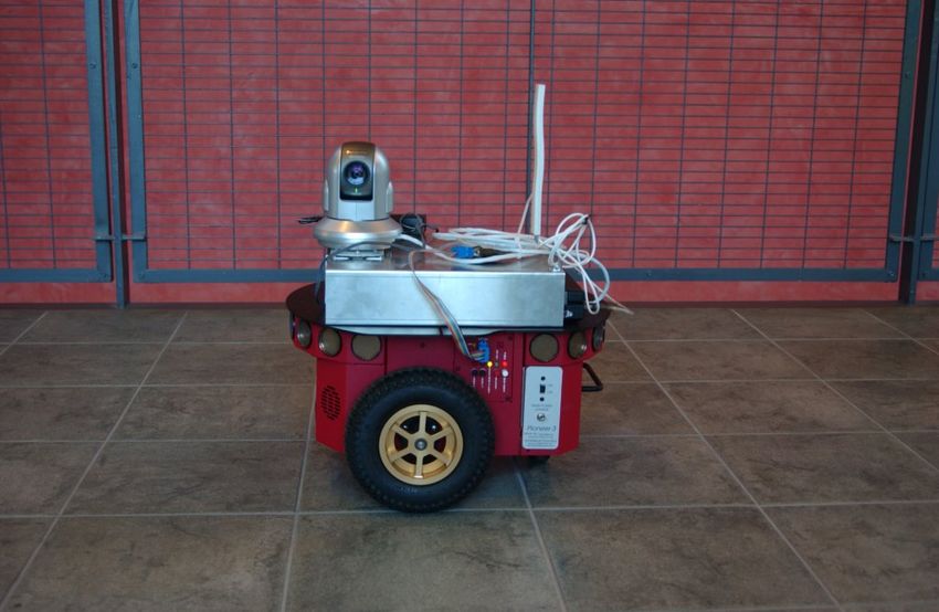
the motors and sonars. P3-DX robot can be seen in figure 12 with a mounted camera
and a WLAN omnidirectional antenna. The camera was not used as a part of localization
system.
Another critical component of the hardware system was the laptop. The laptop used in
conjunction of the robot was a IBM ThinkPad with 1.6 GHz Pentium M processor and
512 MB of memory and Debian Linux as the operating system. The laptop is connected
to the robot using USB converter which converts the data from the laptop USB port to
RS-232 port found in the robot. Default communication interval between the robot and
19Figure 10: Hardware configuration
the laptop running the software is 100 ms. During this time the robot collects data from
sonars and drives the motors according to the instructions from the software. The laptop
is usually hidden in the metal cage seen in figure 12.
Final component used is the WLAN antenna and a PCMCIA WLAN interface card, which
is used with the laptop and the antenna is plugged into the card. This enabled the use of
WLAN measurements in localization while the robot is moving in the environment. The
WLAN interface card is the same that was used in collecting the WLAN RSS maps, what
was done independently from this thesis. This is done to make sure that the RSS maps
match the measurements. Measurements from six different WLAN access points were
used in localization.
4.1.2 Software
On the software side we have software library, which helped in developing the localization
system and the interface to the robot, which is called ARIA. ARIA is a C++-library, which
helps in developing software for the robot and it also includes all the functionality that
the robot needs to be autonomous. Details of the ARIA library will be exlained more
thoroughly in section 4.2.
20Figure 11: Configuration of sonars on P3-DX
Probably the most important tool that was used, was the MobileSim robot simulator,
which allowed development of the localization software without using the robot. This
accelerated the development considerably. Simulator was supplied by the robot manu-
facturer, ActivMedia, LLC. The simulator does not fully represent the real robot, mainly
there are differences with sonar behaviour. The simulator returns always valid readings
from sonars, even though with real sonar the signal could be deflected in a way that it
would not return back to the sensor. Also all of the sonars have new readings after each
communication cycle, which is not the case with real robot as explained before in sec-
tion 4.1.1. This meant that additional steps had to be taken to ensure that localization
works with the real robot as well as the simulator.
Another important tool is Kismet[22], which is a WLAN sniffer. It can detect and mea-
sure RSS from every WLAN client and access point that it can hear through the WLAN
interface. In this thesis, Kismet was used to measure RSS data from access points, which
were previously used in collecting the data for the RSS maps. Kismet itself is only a
server which provides information through it’s TCP server to a client. This was sufficient
functionality. More information about the Kismet server is provided in section 4.2 along
with client implementation.
On the programming side the tool that was used was thr Eclipse IDE[23] as the program-
ming environment. It was chosen, because it provided integrated CVS(Concurrent Ver-
21Figure 12: P3-DX robot
sions System)[24] functionality, and the use of CVS was mandatory. CVS is a SCM(Source
Configuration Management) tool. Although Eclipse was originally developed for Java de-
velopment, it has a plugin, CDT, which enables C++ development.
224.2 Implementation
The implemented software will be explained in the following sections. They cover the
internal structure of the implemented software as well as instructions on how to use the
localization system that was implemented. One of the key points of this section is to
provide information on how the system works so that it can be understood and possibly
modified and expanded in the future. Most important sections considering this are sections
4.2.2 and 4.2.3. The implemented software is currently compatible only with Linux
operating system.
4.2.1 General overview
At first it is useful to get to know the internal structure of the software. A coarse overview
of the entire software can be seen in figure 13. This figure depicts the different software
components that had to be implemented. Arrows show the direction of communication.
The dotted lines represent boundaries between local and remote components. Compo-
nents, which start with the letters "Ar" were already implemented in the ARIA library.
Also it was not necessary to implement the user interface as a suitable user interface "Mo-
bileEyes" was already available from the manufacturer of the robot. This leaves 3 separate
components to be implemented.
Figure 13: Overview of the software implementation
ArRobot component is the most critical component of this system and the Localization
component would not work without it. Basic operation of ArRobot is to send control
commands and receive sensor data(odometry, sonar) from the robot. Tasks which the Ar-
Robot component runs are shown in figure 14. As can be seen from the figure, tasks form
a tree like structure. Server Information Packet(SIP) handler is run first and it invokes the
whole tree as SIPs come from the robot itself. This causes that the entire task tree with
23it’s tasks is run. Default time interval for SIP is 100 ms, meaning that all tasks which are
on the tree should not run for more than 100 ms when running times are combined. This
has had some impact on the design of the Localization component. Order of execution in
the tree is determined by first task type, i.e. the branch. After that the tasks have priority
level ranging from 1 to 100 in individual branches. Figure shows only three branches but
in reality there are two more branches in the tree. These branches are action handling and
state reflection. Action handling handles the internal actions which can be added to this
branch and state reflection updates the robot’s internal information. These two branches
are between the sensor interpretation task and user task branches shown in figure 14.[25]
Figure 14: ArRobot task tree
Different parameters required by the measurement models were estimated by using data
from test runs. Beam range finder model, found in section 3.2.2, parameters were evalu-
ated with a straight run along an office corridor. Ranging data from the sensors was then
evaluated, based on knowledge of approximate width of the corridor. After this, approx-
imate parameters were inputted to the system. WLAN sensor data was collected from a
standstill position using the WLAN antenna on the robot. Data was then evaluated and
parameters, mainly the variance of the Gaussian distribution, were chosen.
244.2.2 Class structure
As the Localization component from figure 13 is by far the most important component, a
simplified class diagram of this component is depicted in figure 15. This diagram shows
the relations between different classes inside the Localization component. Localization
component was implemented as library so that it could be easily put into use independent
of other functions. Each of the classes that were implemented in this component will be
described next, so that their meaning and function is clear.
Most important class of all is the Localization class. Its main functions are to gather data
from various sources, in this case sonar and WLAN data, and to initialize all other classes.
Also it runs each iteration of the MCL at defined time intervals and makes decisions
about the condition of the localization, e.g. if the robot is lost and needs to use global
localization. Localization-class itself has been derived from ArAsyncTask class, which
is provided with the ARIA library. Classes inherited from the ArAsyncTask class can be
run asynchronously, which is the required functionality that the localization of the robot
can run independent of any other component. When created, Localization class adds a
callback function task to the ArRobot task tree. This enables Localization class to read
sensor data(odometry, sonar) from the actual robot each time ArRobot class receives a
SIP from the robot.
ServerInfoLocalization and ServerHandleLocalization classes handle requests from the
user interface. ServerInfoLocalization provides information about the localization, for
example, state and location of the particles used in MCL. ServerHandleLocalization han-
dles change of pose given by user through user interface. This means that that the user can
re-localize the robot at any time and the localization system can handle this by resetting
the robot to the desired position.
ISensorModel and IMotionModel classes in figure 15 are interfaces. Actual models for
MCL can be inherited from these interfaces, motion models from IMotionModel class
and measurement models from ISensorModel. Interfaces use tightly-coupled strategy
design pattern to accommodate future models based on different sensors which are not
used in this thesis. OdometryModel class was inherited from the MotionModel, which
implements the odometry model from section 3.2. Two classes were inherited from the
SensorModel class, BeamRangeFinderModel, for sonar measurement model, and Wlan-
Model, for WLAN RSS model. Explanations for these models can be found in section 3.2.
Methods inside the interface can be called from Localization class when needed for the
25Figure 15: Class diagram of Localization component
MCL algorithm.
PoseSample class is inherited from ArPose class provided within the ARIA library. It
is used to be able to save sample probability along with the pose of the sample. This
helps considerably in communicating between the models and Localization class. Motion
models require the pose of the sample, i.e. hypotesis of the robot pose. Measurement
models require both the pose and probability of the pose so that probability for each
sample can be assigned and accessed in the Localization class.
KismetTCPClient class handles the communication to the Kismet[22] server. The server
offers simple text data to clients. Client can send a text string to the server to request
different types of data. In this system all that was needed was the access points’ MAC
address, its channel and the signal strength from the basestation. KismetTCPClient col-
lects this data and the data can be requested from Localization class to be forwarded to
WlanModel, which is the end user of the data collected from Kismet.
SweepMap class takes the map used in localization and creates a map which covers the
inside of the map. Using this class, Localization class can generate new samples inside the
map, this does not "waste" samples as the robot can only move inside the map. Generating
new samples happens when robot loses localization and needs to use global localization
26or when localization adds new random samples.
LocalizationParameters class handles parameters. Parameters critical to the localization
can be changed from a file and then the parameters are read to the LocalizationParameters
class and then the Localization class can use these values to set parameters for different
models and inside the Localization class itself.
4.2.3 Functionality of Localization library
Flow digrams of the localization component can be seen in figures 16 and 17. Figure 16
shows how the localization component is initialized and figure 17 shows how iterations of
the localization system are carried out. Using these diagrams along with the source code
should help to understand how the localization operates.
Figure 16: Flow chart of initializing localization
The order of operations can be seen from the figure 17. It shows what kind of operations
are used in different conditions. The most important condition is localization success or
failure. At the moment, this condition is triggered, if the amount of samples in the speci-
27Figure 17: Flow chart of localization iteration round
fied zone, more about this zone in section 4.2.5, is less than 10% of the total samples. This
allows multiple, even completely different, robot poses to be kept "alive". The diagram
shows that after 10 failed localization, i.e. 10 failed iterations, WLAN localization is used
on completely new samples, which are distributed randomly inside the map. The num-
ber of new samples is 3000 samples, which gives enough coverage on the map. WLAN
localization assigns probabilities to each of these samples according to the WlanModel
algorithm in figure 8. After this, the samples are resampled to 500 samples, so that only
viable samples are left for the next iteration.
The normal iteration round is simple, the sonar measurement model is used to calculate
sample probabilities and the samples are resampled. After this, a new robot position is
calculated and the robot’s internal state is updated to this acquired pose. However, if the
robot has not moved during the last iteration, the models are not run. Time between the
28iterations has been set to 1 second. This was found suitable to provide good localization
results. More detailed view of the process can be found from the source code. Here the
most important class method is calculating new pose for the robot. This method also
determines if localization has failed or not. It also returns the new pose of the robot. The
pose of the robot is calculated by using the highest probability pose and an average pose
calculated from all the samples inside the zone. Final position is the average between
these poses and the orientation is taken from the average pose. This reduces large sudden
movements of the robot pose.
4.2.4 Documentation
The implemented software was documented with the help of Doxygen[26]. Main features
of Doxygen is that it does not require any external files, only the source files. Documenta-
tion is added to the source files by special comment markings which the Doxygen reads.
Doxygen then adds the comments automatically to the classes. This kind of operation
enables fast documenting of the source code, for example classes and methods, as the
comments can be done at the same time as something new is implemented in the source
files.
Doxygen can create the documentation in many different fileformats, such as Adobe’s
PDF(Portable Document File) through LaTeX files, RTF(Rich Text Format) or HTML(HyperText
Markup Language). Only HTML was used as it can be read using only a web browser.
Documentation can be created using doxygen Doxyfile command from the main
directory, naviloc/localization. The documentation appears under doc/html
directory. Documentation can be then found on each individual class and their individual
methods and variables.
4.2.5 Instructions
Examples of functioning servers for the robot can be found under examples directory.
This directory contains two examples, testServer.cc and testServer2.cc. The
latter example is more complete and offers users the option to relocate the robot. Most
of the example has been taken from ARIA example, guiServer.cpp. Changes have
been made so that it takes into use the implemented software, i.e. Localization library,
29also the navigation functionality has been removed, because SONARNL navigation does
not work without SONARNL localization. Localization functionality is done on lines
120, 265 and 266. On line 120 the Localization object is initialized. On lines 265 and
266 ServerInfoLocalization and ServerHandleLocalization objects are initialized which
connects the server to the localization. Only Localization object is mandatory, but no
information can be passed to UI without ServerInfoLocalization and without ServerHan-
dleLocalization, user cannot control the localization. After the Localization component
has been initialized in the program, it runs without any input from the user.
Compiling the library Localization and the examples can be done by executing
make on the top level directory of localization component, naviloc/localization.
Localization library must be available when example servers are compiled or exe-
cuted.
WLAN localization requires the WLAN RSS maps under naviloc/localization/maps.
The maps have to be grayscale (0-255) PNG(Portable Network Graphics) images. The
names of the images have to be in the following format: "xx_xx_xx_xx_xx_xx.png". The
x’s denote the MAC address of the WLAN access point. If these conditions are fulfilled,
the rest of the process is automated.
Under directory params there is a file called localization.p. This file controls
some of the important localization parameters. There are currently 17 parameters. Next,
all the parameters and their effect on localization will be explained. Parameter names are
written with fixed-width font.
NumSamples controls the amount of samples used in localization. More samples mean
better localization result, but it also increases computing time. ZoneSize controls the
size of the zone which is placed on top of the most probable sample after each itera-
tion. If enough samples are within the zone the localization is considered successful.
ZoneSize parameter defines half of the width of a square, side of the square is 2 times
ZoneSize. Parameter wFast defines coefficient for calculating short-term average re-
sult of the localization. Parameter wSlow in the otherhand defines coefficient for cal-
culating long-term average result of the localization. These two last parameters have
relation wF ast >> wSlow ≥ 0. All these parameters control general behaviour of the
localization system.
Next parameters affect the Odometry model of the localization system. Alpha1, Alpha2,
Alpha3 and Alpha4 correspond to the α1 , α2 , α3 and α4 parameters in the algorithm 5.
30You can also read