Modeling Natural Images Using Gated MRFs
←
→
Page content transcription
If your browser does not render page correctly, please read the page content below
JOURNAL OF PAMI, VOL. ?, NO. ?, JANUARY 20??                                                                                                 1

    Modeling Natural Images Using Gated MRFs
              Marc’Aurelio Ranzato, Volodymyr Mnih, Joshua M. Susskind, Geoffrey E. Hinton

      Abstract—This paper describes a Markov Random Field for real-valued image modeling that has two sets of latent variables.
      One set is used to gate the interactions between all pairs of pixels while the second set determines the mean intensities of each
      pixel. This is a powerful model with a conditional distribution over the input that is Gaussian with both mean and covariance
      determined by the configuration of latent variables, which is unlike previous models that were restricted to use Gaussians with
      either a fixed mean or a diagonal covariance matrix. Thanks to the increased flexibility, this gated MRF can generate more realistic
      samples after training on an unconstrained distribution of high-resolution natural images. Furthermore, the latent variables of
      the model can be inferred efficiently and can be used as very effective descriptors in recognition tasks. Both generation and
      discrimination drastically improve as layers of binary latent variables are added to the model, yielding a hierarchical model called
      a Deep Belief Network.

      Index Terms—gated MRF, natural images, deep learning, unsupervised learning, density estimation, energy-based model,
      Boltzmann machine, factored 3-way model, generative model, object recognition, denoising, facial expression recognition

                                                                       F

1    I NTRODUCTION                                                         that can be used for image restoration tasks [10], [11],
                                                                           [12]. Thanks to their generative ability, probabilistic models
T    HE   study of the statistical properties of natural images
     has a long history and has influenced many fields, from
image processing to computational neuroscience [1]. In
                                                                           can cope more naturally with ambiguities in the sensory
                                                                           inputs and have the potential to produce more robust
computer vision, for instance, ideas and principles derived                features. Devising good models of natural images, however,
from image statistics and from studying the processing                     is a challenging task [1], [12], [13], because images are
stages of the human visual system have had a significant                   continuous, high-dimensional and very highly structured.
impact on the design of descriptors that are useful for                       Recent studies have tried to capture high-order dependen-
discrimination. A common paradigm has emerged over the                     cies by using hierarchical models that extract highly non-
past few years in object and scene recognition systems.                    linear representations of the input [14], [15]. In particular,
Most methods [2] start by applying some well-engineered                    deep learning methods construct hierarchies composed of
features, like SIFT [3], HoG [4], SURF [5], or PHoG [6], to                multiple layers by greedily training each layer separately
describe image patches, and then aggregating these features                using unsupervised algorithms [8], [16], [17], [18]. These
at different spatial resolutions and on different parts of the             methods are appealing because 1) they adapt to the input
image to produce a feature vector which is subsequently fed                data; 2) they recursively build hierarchies using unsu-
into a general purpose classifier, such as a Support Vector                pervised algorithms, breaking up the difficult problem of
Machine (SVM). Although very successful, these methods                     learning hierarchical non-linear systems into a sequence
rely heavily on human design of good patch descriptors                     of simpler learning tasks that use only unlabeled data; 3)
and ways to aggregate them. Given the large and growing                    they have demonstrated good performance on a variety
amount of easily available image data and continued ad-                    of domains, from generic object recognition to action
vances in machine learning, it should be possible to exploit               recognition in video sequences [17], [18], [19].
the statistical properties of natural images more efficiently                 In this paper we propose a probabilistic generative
by learning better patch descriptors and better ways of                    model of images that can be used as the front-end of a
aggregating them. This will be particularly significant for                standard deep architecture, called a Deep Belief Network
data where human expertise is limited such as microscopic,                 (DBN) [20]. We test both the generative ability of this
radiographic or hyper-spectral imagery.                                    model and the usefulness of the representations that it learns
   In this paper, we focus on probabilistic models of natural              for applications such as object recognition, facial expression
images which are useful not only for extracting represen-                  recognition and image denoising, and we demonstrate state-
tations that can subsequently be used for discriminative                   of-the-art performance for several different tasks involving
tasks [7], [8], [9], but also for providing adaptive priors                several different types of image.
                                                                              Our probabilistic model is called a gated Markov Ran-
• M. Ranzato, V. Mnih and G.E. Hinton are with the Department of           dom Field (MRF) because it uses one of its two sets of
  Computer Science, University of Toronto, Toronto, ON, M5S 3G4,           latent variables to create an image-specific energy function
  CANADA.
  E-mail: see http://www.cs.toronto.edu/˜ranzato
                                                                           that models the covariance structure of the pixels by switch-
• J.M. Susskind is with Machine Perception Laboratory, University of       ing in sets of pairwise interactions. It uses its other set of
  California San Diego, La Jolla, 92093, U.S.A.                            latent variables to model the intensities of the pixels [13].
                                                                           The DBN then uses several further layers of Bernoulli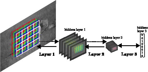
JOURNAL OF PAMI, VOL. ?, NO. ?, JANUARY 20??                                                                                         2

latent variables to model the statistical structure in the       x2                       x2                     x2
hidden activities of the two sets of latent variables of the
gated MRF. By replicating features in the lower layers it
is possible to learn a very good generative model of high-
resolution images and to use this as a principled framework            PCA                     PPCA                   FA
for learning adaptive descriptors that turn out to be very                           x1                     x1                      x1
useful for discriminative tasks.                                 x2                       x2                     x2
   In the reminder of this paper, we first discuss our new
contributions with respect to our previous published work
and then describe the model in detail. In sec. 2 we review
other popular generative models of images and motivate                                         PoT                    mPoT
                                                                       SC
the need for the model we propose, the gated MRF. In
sec. 3, we describe the learning algorithm as well as the                           x1                     x1                     x1
inference procedure for the gated MRF. In order to capture       Fig. 1. Toy illustration to compare different models. x-axis is the
                                                                 first pixel, y-axis is the second pixel of two-pixel images. Blue dots
the dependencies between the latent variables of the gated       are a dataset of two-pixel images. The red dot is the data point we
MRF, several other layers of latent variables can be added,      want to represent. The green dot is its (mean) reconstruction. The
yielding a DBN with many layers, as described in sec. 4.         models are: Principal Component Analysis, Probabilistic PCA, Factor
                                                                 Analysis, Sparse Coding, Product of Student’s t and mean PoT.
Such models cannot be scaled in a simple way to deal with
high-resolution images because the number of parameters
scales quadratically with the dimensionality of the input at     underlying assumptions limit their modeling abilities. This
each layer. Therefore, in sec. 5 an efficient and effective      motivates the introduction of the model we propose. After
weight-sharing scheme is introduced. The key idea is to          describing our basic model and its learning and inference
replicate parameters across local neighborhoods that do          procedures, we show how we can make it hierarchical and
not overlap in order to accomplish a twofold goal: exploit       how we can scale it up using parameter-sharing to deal with
stationarity of images while limiting the redundancy of          high-resolution images.
latent variables encoding features at nearby image locations.
Finally, we present a thorough validation of the model in
sec. 6 with comparisons to other models on a variety of          2.1    Relation to Other Probabilistic Models
image types and tasks.                                           Natural images live in a very high dimensional space that
                                                                 has as many dimensions as number of pixels, easily in the
1.1 Contributions                                                order of millions and more. Yet it is believed that they
This paper is a coherent synthesis of previously unpublished     occupy a tiny fraction of that space, due to the structure
results with the authors’ previous work on gated MRFs [21],      of the world, encompassing a much lower dimensional
[9], [13], [22] that has appeared in several recent conference   yet highly non-linear manifold [23]. The ultimate goal of
papers and is intended to serve as the main reference on the     unsupervised learning is to discover representations that pa-
topic, describing in a more organized and consistent way         rameterize such a manifold, and hence, capture the intrinsic
the major ideas behind this probabilistic model, clarifying      structure of the input data. This structure is represented
the relationship between the mPoT and mcRBM models               through features, also called latent variables in probabilistic
described below, and providing more details (including           models.
pseudo-code) about the learning algorithms and the exper-           One simple way to check whether a model extracts
imental evaluations. We have included a subsection on the        features that retain information about the input, is by recon-
relation to other classical probabilistic models that should     structing the input itself from the features. If reconstruction
help the reader better understand the advantages of the          errors of inputs similar to training samples is lower than
gated MRF and the similarities to other well-known models.       reconstruction errors of other input data points, then the
The paper includes empirical evaluations of the model on         model must have learned interesting regularities [24]. In
an unusually large variety of tasks, not only on an image        PCA, for instance, the mapping into feature space is a linear
denoising and generation tasks that are standard ways to         projection into the leading principal components and the
evaluate probabilistic generative models of natural images,      reconstruction is performed by another linear projection.
but also on three very different recognition tasks (scenes,      The reconstruction is perfect only for those data points that
generic object recognition, and facial expressions under         lie in the linear subspace spanned by the leading principal
occlusion). The paper demonstrates that the gated MRF can        components. The principal components are the structure
be used for a wide range of different vision tasks, and it       captured by this model.
should suggest many other tasks that can benefit from the           Also in a probabilistic framework we have a mapping
generative power of the model.                                   into feature, or latent variable, space and back to image
                                                                 space. The former is obtained by using the posterior
2    T HE G ATED MRF                                             distribution over the latent variables, p(h|x) where x is
In this section, we first review some of the most popu-          the input and h the latent variables, the latter through the
lar probabilistic models of images and discuss how their         conditional distribution over the input, p(x|h).
JOURNAL OF PAMI, VOL. ?, NO. ?, JANUARY 20?? 3
As in PCA one would reconstruct the input from the
features in order to assess the quality of the encoding,
while in a probabilistic setting we can analyze and compare
different models in terms of their conditional p(x|h). We
can sample the latent variables, h̄ ∼ p(h|x̄) given an input
image x̄, and then look at how well the image x̄ can be
reconstructed using p(x|h̄). Reconstructions produced in
this way are typically much more like real data than true
samples from the underlying generative model because the
latent variables are sampled from their posterior distribu-
tion, p(h|x̄), rather than from their prior, p(h), but the
reconstructions do provide insight into how much of the
information in the image is preserved in the sampled values
of the latent variables.
As shown in fig. 1, most models such as Probabilistic
Principal Component Analysis (PPCA) [25], Factor Analy-
sis (FA) [26], Independent Component Analysis (ICA) [27], Fig. 2. In the first column, each image is zero mean. In the
Sparse Coding (SC) [28], and Gaussian Restricted Boltz- second column, the whole data set is centered but each image
mann Machines (GRBM) [29], assume that the conditional can have non-zero mean. First row: 8x8 natural image patches and
contours of the empirical distribution of (tiny) two-pixel images (the
distribution of the pixels p(x|h) is Gaussian with a mean x-axis being the first pixel and the y-axis the second pixel). Second
determined by the latent variables and a fixed, image- row: images generated by a model that does not account for mean
independent covariance matrix. In PPCA the mean of intensity with plots of how such model could fit the distribution of
two-pixel images using mixture of Gaussians with components that
the distribution lies along the directions of the leading can choose between two covariances. Third row: images generated
eigenvectors while in SC it is along a linear combination by a model that has both “mean” and “covariance” hidden units and
of a very small number of basis vectors (represented by toy-illustration of how such model can fit the distribution of two-pixel
images discovering the manifold of structured images (along the anti-
black arrows in the figure). From a generative point of view, diagonal) using a mixture of Gaussians with arbitrary mean and only
these are rather poor assumptions for modeling natural two covariances.
images because much of the interesting structure of natural
images lies in the fact that the covariance structure of the
tied parameters.
pixels varies considerably from image to image. A vertical
occluding edge, for example, eliminates the typical strong
correlation between pixels on opposite sides of the edge. 2.2 Motivation
This limitation is addressed by models like Product of A Product of Student’s t (PoT) model [31] can be viewed as
Student’s t (PoT) [30], covariance Restricted Boltzmann modelling image-specific, pair-wise relationships between
Machine (cRBM) [21] and the model proposed by Karklin pixel values by using the states of its latent variables. It
and Lewicki [14] each of which instead assume a Gaussian is very good at representing the fact that two pixels have
conditional distribution with a fixed mean but with a full very similar intensities and no good at all at modelling what
covariance determined by the states of the latent vari- these intensities are. Failure to model the mean also leads
ables. Latent variables explicitly account for the correlation to impoverished modelling of the covariances when the
patterns of the input pixels, avoiding interpolation across input images have non-zero mean intensity. The covariance
edges while smoothing within uniform regions. The mean, RBM (cRBM) [21] is another model that shares the same
however, is fixed to the average of the input data vectors limitation since it only differs from PoT in the distribution
across the whole dataset. As shown in the next section, of its latent variables: The posterior over the latent variables
this can yield very poor conditional models of the input p(h|x) is a product of Bernoulli distributions instead of
distribution. Gamma distributions as in PoT.
In this work, we extend these two classes of models with We explain the fundamental limitation of these models
a new model whose conditional distribution over the input by using a simple toy example: Modelling two-pixel images
has both a mean and a covariance matrix determined by using a cRBM with only one binary latent variable (see
latent variables. We will introduce two such models, namely fig. 2). This cRBM assumes that the conditional distribution
the mean PoT (mPoT) [13] and the mean-covariance RBM over the input p(x|h) is a zero-mean Gaussian with a
(mcRBM) [9], which differ only in the choice of their covariance that is determined by the state of the latent
distribution over latent variables. We refer to these models variable. Since the latent variable is binary, the cRBM can
as gated MRF’s because they are pair-wise Markov Random be viewed as a mixture of two zero-mean full covariance
Fields (MRFs) with latent variables gating the couplings Gaussians. The latent variable uses the pairwise relationship
between input variables. Their marginal distribution can between pixels to decide which of the two covariance
be interpreted as a mixture of Gaussians with an infinite matrices should be used to model each image. When the
(mPoT) or exponential (mcRBM) number of components, input data is pre-processed by making each image have zero
each with non-zero mean and full covariance matrix and mean intensity (the plot of the empirical histogram is shownJOURNAL OF PAMI, VOL. ?, NO. ?, JANUARY 20?? 4
in the first row and first column), most images lie near the latent variables are denoted by the vector hp ∈ {0, 1}N .
origin because most of the times nearby pixels are strongly First, we consider a pair-wise MRF defined in terms of
correlated. Less frequently we encounter edge images that an energy function E. The probability density function is
exhibit strong anti-correlation between the pixels, as shown related to E by: p(x, hp ) = exp(−E(x, hp ))/Z, where Z
by the long tails along the anti-diagonal line. A cRBM is an (intractable) normalization constant which is called
could model this data by using two Gaussians (second row the partition function. The energy is:
and first column): one that is spherical and tight at the origin 1X
for smooth images and another one that has a covariance E(x, hp ) = tijk xi xj hpk (1)
2
elongated along the anti-diagonal for structured images. i,j,k
If, however, the whole set of images is normalized The states of the latent variables, called precision hidden
by subtracting from every pixel the mean value of all units, modulate the pair-wise interactions tijk between all
pixels over all images (first row and second column), the pairs of input variables xi and xj , with i, j = 1..D. Sim-
cRBM fails at modelling structured images (second row ilarly to Sejnowski [32], the energy function is defined in
and second column). It can fit a Gaussian to the smooth terms of 3-way multiplicative interactions. Unlike previous
images by discovering the direction of strong correlation work by Memisevic and Hinton [33] on modeling image
along the main diagonal, but it is very likely to fail to transformations, here we use this energy function to model
discover the direction of anti-correlation, which is crucial the joint distribution of the variables within the vector x.
to represent discontinuities, because structured images with This way of allowing hidden units to modulate inter-
different mean intensity appear to be evenly spread over the actions between input units has far too many parameters.
whole input space. For real images we expect the required lateral interactions
If the model has another set of latent variables that to have a lot of regular structure. A hidden unit that
can change the means of the Gaussian distributions in the represents a vertical occluding edge, for example, needs
mixture (as explained more formally below and yielding to modulate the lateral interactions so as to eliminate
the mPoT and mcRBM models), then the model can rep- horizontal interpolation of intensities in the region of the
resent both changes of mean intensity and the correlational edge. This regular structure can be approximated by writing
structure of pixels (see last row). The mean latent variables the 3-dimensional tensor of parameters t as a sum of outer
P (1) (2)
effectively subtract off the relevant mean from each data- products: tijk = f Cif Cjf Pf k , where f is an index
point, letting the covariance latent variable capture the over F deterministic factors, C (1) and C (2) ∈ RD×F , and
covariance structure of the data. As before, the covariance P ∈ RF ×N . Since the factors are connected twice to the
latent variable needs only to select between two covariance same image through matrices C (1) and C (2) , it is natural to
matrices. tie their weights further reducing the number Pof parameters,
In fact, experiments on real 8x8 image patches confirm yielding the final parameterization tijk = f Cif Cjf Pf k .
these conjectures. Fig. 2 shows samples drawn from PoT Thus, taking into account also the hidden biases, eq. 1
and mPoT. The mPoT model (and similarly mcRBM [9]) becomes:
is better at modelling zero mean images and much better F N D N
1X X X X
at modelling images that have non-zero mean intensity. E(x, hp ) = ( Pf k hpk )( Cif xi )2 − bpk hpk (2)
This will be particularly relevant when we introduce a 2 i=1
f =1 k=1 k=1
convolutional extension of the model to represent spatially which can be written more compactly in matrix form as:
stationary high-resolution images (as opposed to small im-
1
age patches), since it will not be possible to independently E(x, hp ) = xT Cdiag(P hp )C T x − bp T hp (3)
normalize overlapping image patches. 2
As we shall see in sec. 6.1, models that do not account where diag(v) is a diagonal matrix with diagonal entries
for mean intensity cannot generate realistic samples of given by the elements of vector v. This model can be
natural images since samples drawn from the conditional interpreted as an instance of an RBM modeling pair-
distribution over the input have expected intensity that is wise interactions between the input pixels1 and we dub it
constant everywhere regardless of the value of the latent covariance RBM (cRBM) [21], [9]2 since it models the
variables. In the model we propose instead there is a set covariance structure of the input through the “precision”
of latent variables whose role is to bias the average mean latent variables hp .
intensity differently in different regions of the input image. The hidden units remain conditionally independent given
Combined with the correlational structure provided by the the states of the input units and their binary states can be
covariance latent variables, this produces smooth images sampled using:
that have sharp boundaries between regions of different
1X
F X D
mean intensity. p(hpk = 1|x) = σ − Pf k ( Cif xi )2 + bpk (4)
2 i=1
f =1
2.3 Energy Functions 1. More precisely, this is an instance of a semi-restricted Boltzmann
machine [34], [35], since only hidden units are “restricted”, i.e. lack lateral
We start the discussion assuming the input is a small interactions.
vectorized image patch, denoted by x ∈ RD , and the 2. This model should not be confused with the conditional RBM [36].JOURNAL OF PAMI, VOL. ?, NO. ?, JANUARY 20?? 5
where σ is the logistic function σ(v) = 1/ 1 + exp(−v) . precision
factors mean units
units
Given the states of the hidden units, the input units form pixels
an MRF in which the effective
P P pairwise interaction weight
between xi and xj is 21 f k Pf k hpk Cif Cjf . Therefore, N F M
the conditional distribution over the input is:
p(x|hp ) = N (0, Σ), with Σ−1 = Cdiag(P hp )C T (5) Fig. 3. Graphical model representation (with only three input
variables): There are two sets of latent variables (the mean and the
Notice that the covariance matrix is not fixed, but is a precision units) that are conditionally independent given the input
function of the states of the precision latent variables hp . pixels and a set of deterministic factor nodes that connect triplets of
In order to guarantee positive definiteness of the covariance variables (pairs of input variables and one precision unit).
matrix we need to constrain P to be non-negative and add a
small quadratic regularization term to the energy function3 ,
here ignored for clarity of presentation.
As described in sec. 2.2, we want the conditional dis-
tribution over the pixels to be a Gaussian with not only
its covariance but also its mean depending on the states of
the latent variables. Since the product of a full covariance Fig. 4. A) Input image patch. B) Reconstruction performed using
Gaussian (like the one in eq. 5) with a spherical non- only mean hiddens (i.e. W hm + bx ) (top) and both mean and preci-
zero mean Gaussian is a non-zero mean full covariance sion hiddens (bottom) (that is multiplying the patch on the top by the
−1
image-specific covariance Σ = Cdiag(P hp )C T + I , see mean
Gaussian, we simply add the energy function of cRBM in of Gaussian in eq. 7). C) Reconstructions produced by combining the
eq. 3 to the energy function of a GRBM [29], yielding: correct image-specific covariance as above with the incorrect, hand-
specified pixel intensities shown in the top row. Knowledge about
1 T
E(x, hm , hp ) = x Cdiag(P hp )C T x − bp T hp pair-wise dependencies allows a blob of high or low intensity to be
spread out over the appropriate region. D) Reconstructions produced
2
1 like in C) showing that precision hiddens do not account for polarity
+ xT x − hm W T x − bm T hm − bx T x (6) (nor for the exact intensity values of regions) but only for correlations.
2
where hm ∈ {0, 1}M are called “mean” latent variables be-
cause they contribute to control the mean of the conditional For instance, it knows that the pixels in the lower part of
distribution over the input: the image in fig. 4-A are strongly correlated; these pixels
are likely to take the same value, but the precision latent
p(x|hm , hp ) = N Σ(W hm + bx ), Σ , (7) variables do not carry any information about which value
this is. Then, very noisy information about the values of the
with Σ−1 = Cdiag(P hp )C T + I individual pixels in the lower part of the image, as those
where I is the identity matrix, W ∈ RD×M is a matrix of provided by the mean latent variables, would be sufficient
trainable parameters and bx ∈ RD is a vector of trainable to reconstruct the whole region quite well, since the model
biases for the input variables. The posterior distribution knows which values can be smoothed. Mathematically, the
over the mean latent variables is4 : interaction between mean and precision latent variables
is expressed by the product between Σ (which depends
D
X only on hp ) and W hm + bx in the mean of the Gaussian
p(hm
k = 1|x) = σ( Wik xi + bm
k ) (8)
distribution of eq. 7. We can repeat the same argument
i=1
for the pixels in the top right corner and for those in the
The overall model, whose joint probability
density function middle part of the image as well. Fig. 4-C illustrates this
is proportional to exp(−E x, hm , hp ) , is called a mean concept, while fig. 4-D shows that flipping the sign of
covariance RBM (mcRBM) [9] and is represented in fig. 3. the reconstruction of the mean latent variables flips the
sign of the overall reconstruction as expected. Information
The demonstration in fig. 4 is designed to illustrate about intensity is propagated over each region thanks to the
how the mean and precision latent variables cooperate to pair-wise dependencies captured by the precision hidden
represent the input. Through the precision latent variables units. Fig. 4-B shows the same using the actual mean
the model knows about pair-wise correlations in the image. intensity produced by the mean hidden units (top). The
reconstruction produced by the model using the whole set
3. In practice, this term is not needed when the dimensionality of hp
is larger than x. of hidden units is very close to the input image, as can be
4. Notice how the mean latent variables compute a non-linear projection seen in the bottom part of fig. 4-B.
of a linear filter bank, akin to the most simplified “simple-cell” model In a mcRBM the posterior distribution over the latent
of area V1 of the visual cortex, while the precision units perform an
operation similar to the “complex-cell” model because rectified (squared) variables p(h|x) is a product of Bernoullis as shown in
filter outputs are non-linearly pooled to produce their response. In this eq. 8 and 4. This distribution is particularly easy to use
model, simple and complex cells perform their operations in parallel (not in a standard DBN [20] where each layer is trained using
sequentially). If, however, we equate the factors used by the precision
units to simple cells, we recover the standard model in which simple cells a binary-binary RBM. Binary latent variables, however,
send their squared outputs to complex cells. are not very good at representing different real-values ofJOURNAL OF PAMI, VOL. ?, NO. ?, JANUARY 20?? 6
the mean intensity or different levels of contrast across an quadratic in the filter output value. This leads to sparse
edge. A binary latent variable can represent a probability filter outputs that are usually close to zero but occasionally
of 0.71 that a binary feature is present, but this is not at much larger. By default hidden units are all “on” because
all the same as representing that a real-valued intensity the input is not typically aligned with the oriented filters,
is 0.71 and definitely not 0.70 or 0.72. In our previous but when an input x matches a filter, the corresponding
work [21] we showed that by combining many binary hidden unit turns “off” thus representing the violation of a
variables with shared weights and offset biases we can smoothness constraint.
closely approximate continuous Gamma units, however. In other words, images are assumed to be almost always
This issue can be addressed in several other ways, by either smooth, but rare violations of this constraint are allowed
normalizing the input data x, or by normalizing the input by using auxiliary (latent) variables that act like switches.
in the energy function [9], or by changing the distribution This idea was first proposed by Geman and Geman [39] and
of the latent variables. later revisited by many others [40], [41]. Like the Gaussian
In our experiments, we tried a few distributions5 and Scale Mixture model [10], our model uses hidden variables
found that Bernoulli variables for the mean hiddens and that control the modeled covariance between pixels, but
Gamma variables for the precision hiddens gave the best our inference process is simpler because the model is
generative model. The resulting model, dubbed mean PoT undirected. Also, all parameters of our model are learned.
(mPoT), is a slight modification of mcRBM. The energy
is: 2.5 Notes on the Modelling Choice
1 As stated in sec. 2.2, the main motivation for the model
E(x, hm , hp ) = xT Cdiag(P hp )C T x + 1T (hp + we propose is to define a conditional distribution over the
2
1 T input p(x|hm , hp ) which is a multivariate Gaussian with
(1 − γ) log h ) + x x − hm W T x − bm T hm − bx T x (9)
p
both mean and covariance determined by the state of latent
2
variables. In order to achieve this, we have defined an
where 1 is a vector of 1’s, γ ∈ R+ and hp is a positive
energy function of the type: E = 21 xT Σ−1 hp x + Wh x,
m
vector of real valued variables [31]. In mPoT the posterior
where we denote with Σh and Wh matrices that depend
p m
distribution over the precision hiddens is:
on hp and hm , respectively. Two questions naturally arise.
1X X First, would the model work as well if we tie the set of
p(hpj |x) = Γ(γ, 1 + Pf j ( Cif xi )2 ) (10)
2 latent variables that control the mean and covariance? And
f i
second, are there other formulations of energy functions
where Γ is the Gamma distribution with expected value: that define multivariate Gaussian conditional distributions?
γ The answer to the first question is negative for a model
E[hpj |x] = (11) of natural images since the statistics of the covariance
1 + 12 f Pf j ( i Cif xi )2
P P
structure is heavy tailed (nearby pixels are almost always
Compared to eq. 4, we see that the operations required strongly correlated) while the statistics of the mean in-
to compute the expectations are very similar, except for tensity is not. This affects the statistics of the mean and
the non-linear transformation on the pooled squared filter covariance latent variables as well. The former is typically
outputs. much sparser than the latter, therefore, tying both sets of
latent variables would constrain the model in an unnatural
2.4 Relation to Line Processes and Sparse Cod- way.
ing The answer to the second question is positive instead.
The alternative would be the following energy function:
Let us consider the energy function of eq. 2 assuming
E = 21 (x − Whm )T Σ−1 hp (x − Wh ). The advantage of this
m
that P is set to identity and the biases are all large and
formulation is that the parameters defining the mean are
positive. The energy penalizes those images x that yield
defined in the image domain and, therefore, are much easier
large filter responses (because of the positive sign of the
to interpret. The mean parameters directly define the mean
energy function) [37]. Without latent variables that have
of the Gaussian distribution, while in our formulation the
the possibility of turning off, the model would discover the
mean of the Gaussian distribution is given by a product,
minor components of the data [38], i.e. the filter weights
Σhp Whm , see eq. 7. The fundamental disadvantage of this
would represent the directions of the minor components or
formulation is that inference of the latent variables becomes
linear combinations of those directions. The introduction of
inefficient since the energy function has multiplicative
latent variables makes the model highly non-linear, causing
interactions between latent variables which make them
it to learn filters with heavy-tailed output distributions. In
conditionally dependent given the input. Lengthy iterative
the rare event of a non-smooth image (e.g., an edge in a
procedures would be required to compute a sample from
certain location and orientation), a large filter output will
p(hm |x) and p(hp |x).
cause the corresponding latent variable to turn off so that
the increase in energy is equal to the bias rather than 3 L EARNING A LGORITHM
5. An extensive evaluation of different choices of latent variable distri- The models described in the previous section can be re-
butions is not explored here, and it is subject of future study. formulated by integrating out the latent variables over theirJOURNAL OF PAMI, VOL. ?, NO. ?, JANUARY 20?? 7
def train_DBN():
domain. In the case of mPoT,
R forPinstance, we have that the # loop from bottom to top layer
free energy F(x) = − log hp hm exp(−E(x, hm , hp )) for k in range(number_of_layers):
W[k] = random_init()
is: Wf[k] = 0 # fast weights used by FPCD
neg_batch = random_init() # init. samples from model
N F D D # sweep over data divided into minibatches
X 1X X X 1 2
F(x) = log(1 + Pf j ( Cif xi )2 ) + x for epoch in range(number_of_epochs):
j=1
2 i=1 i=1
2 i for batch in range(number_of_minibatches):
f =1 g1 = compute_dFdW(batch,W[k])
D M neg_batch = draw_sample(neg_batch,W[k]+Wf[k],k)
Wik xi +bm
X X P
g2 = compute_dFdW(neg_batch,W[k]+Wf[k])
− bxi xi − log(1 + e i k ) (12) W[k] = W[k] - (learn_rate/epoch)*(g1-g2 + decay*W[k])
i=1 k=1 Wf[k] = 19/20*Wf[k] - learn_rate*(g1-g2)
# make minibatches for layer above by computing E[h|x]
making the marginal distribution, p(x) ∝ exp(−F(x)), a generate_data_using_posterior(batches,W[k])
product of experts [42].
Let us denote a generic parameter of the model with def draw_sample(datainit,param,layer): # only 1 M.C. step
if layer == 1: # 1st layer: do 1 step of HMC
θ ∈ {C, P, γ, W, bx , bm }. We learn the parameters by velocity = randn()
stochastic gradient ascent in the log likelihood. We can tot_energy1 = .5*velocityˆ2 + compute_F(datainit,param)
data = datainit
write the likelihood in terms of the joint energy E or in velocity = velocity - eps * compute_dFdX(data,param)/2
terms of the free energy F. In both cases, maximum like- for iter in range(20): # 20 leap-frog steps
data = data + eps * velocity
lihood requires us to compute expectations over the model if iter != 19:
distributions. These can be approximated with Monte Carlo velocity = velocity - eps * compute_dFdX(data,param)
velocity = velocity - eps * compute_dFdX(data,param)
sampling algorithms. When using E the most natural sam- tot_energy2 = .5*velocityˆ2 + compute_F(data,param)
pling algorithm is Gibbs sampling (alternating the sampling if rand() < exp(tot_energy1 - tot_energy2):
return data # accept sample
from p(hm |x) and p(hp |x) to p(x|hm , hp )), while Hybrid else:
Monte Carlo (HMC) [43] is a better sampling algorithm return datainit # reject sample
else: # higher layers: do 1 step of Gibbs
when using F since x ∈ RD and F is differentiable. It hiddens = sample_posterior(datainit,param) # p(h|x)
is beyond the scope of this work to analyze and compare return sample_inputs(hiddens,param) # p(x|h)
different sampling methods. Our preliminary experiments Fig. 5. Pseudo-code of learning algorithm for DBN using FPCD.
showed that training with HMC yielded models that pro- Energy function given by eq. 12.
duce better visually looking samples, and therefore, we will
now describe the algorithm in terms F only.
The update rule for gradient ascent in the likelihood is: running HMC for just one set of 20 leap-frog steps (using
the slightly perturbed parameter vector in the free energy
∂F ∂F
θ ←θ+η < > −< > (13) function), (3) it computes < ∂F
∂θ > at the negative samples,
∂θ model ∂θ data and (4) it updates the parameters using eq. 13 (see algorithm
where denotes expectation over samples from the in fig. 5).
model or the training data. While it is straightforward to
compute the value and the gradient of the free energy with
respect to θ, computing the expectations over the model 4 L EARNING A DBN
distribution is intractable because we would need to run the In their work, Hinton et al. [20] trained DBNs using a
HMC sampler for a very long time, discarding and reinitial- greedy layer-wise procedure, proving that this method, if
izing the momentum auxiliary variables many times [43]. done properly, creates a sequence of lower bounds on the
We approximate that with Fast Persistent Contrastive Di- log likelihood of the data, each of which is better than the
vergence (FPCD) [44]. We run the sampler for only one previous bound. Here, we follow a similar procedure. First,
step6 starting at the previous sample drawn from the model we train a gated MRF to fit the distribution of the input.
and using as parameters the sum of the original parameters Then, we use it to compute the expectation of the first layer
and a small perturbation vector which adapts rapidly but latent variables conditioned on the input training images.
also decays towards zero rapidly. The perturbation vector Second, we use these expected values as input to train the
repels the system from its current state by raising the second layer of latent variables7 . Once the second layer is
energy of that state and it therefore encourages samples trained, we use it to compute expectations of the second
to explore the input space rapidly even when the learning layer latent variables conditioned on the second layer input
rate for the model parameters is very small (see [44] for to provide inputs to the third layer, and so on. The difficult
more details). The learning algorithm loops over batches problem of learning a hierarchical model with several layers
of training samples and: (1) it computes < ∂F ∂θ > at the
training samples, (2) it generates “negative” samples by 7. It would be more correct to use stochastically sampled values as
the “data”, but using the expectations reduces noise in the learning and
6. One step of HMC is composed of a randomly chosen initial mo- works almost as well. Also, the second layer RBM expects input values
mentum and 20 “leap-frog steps” that follow a dynamical simulation. If in the interval [0, 1] when using the expectations of Bernoulli variables.
the sum of the kinetic and potential energy rises by ∆ due to inaccurate Therefore, when we use the precision units of mPoT, we divide the
simulation of the dynamics, the system is returned to the initial state with expectation of eq. 11 by γ. A more elegant solution is to change the
probability 1 − exp(−∆). The step size of the simulation is adjusted to conditional distribution in the second layer RBM to Gamma. However,
keep the rejection rate at 10%. the simple rescaling worked well in our experiments.JOURNAL OF PAMI, VOL. ?, NO. ?, JANUARY 20?? 8
of latent variables is thus decomposed into a sequence of
much simpler learning tasks.
Let us consider the i-th layer of the deep model in
isolation. Let us assume that the input to that layer consists
of a binary vector denoted by hi−1 ∈ {0, 1}Ni−1 . This is
modeled by a binary RBM which is also defined in terms
of an energy function:
T T T
E(hi−1 , hi ) = −hi−1 W i hi − bi−1 hi−1 − bi hi (14)
where W i ∈ RNi−1 ×Ni is the i-th layer parameter matrix Fig. 6. Outline of a deep generative model composed of three
and bi ∈ RNi is the i-th layer vector of biases. In a RBM, layers. The first layer applies filters that tile the input image with
different offsets (squares of different color are filters with different
all input variables are conditionally independent given the parameters). The filters of this layer are learned on natural images.
latent variables and vice versa; so: Afterwards, a second layer is added using as input the expectation
Ni−1
of the first layer latent variables. This layer is trained to fit the
X
i i−1
distribution of its input. The procedure is repeated again for the third
p(hik i−1
= 1|h ) = σ( Wjk hj + bik ), k = 1..Ni (15) layer. After training, inference of the top level representation is well
j=1 approximated by propagating the expectation of the latent variables
given their input starting from the input image (see dashed arrows).
Ni
X Generation is performed by first using a Monte Carlo method to
p(hji−1 = 1|hi ) = σ( i i
Wjk hk + bi−1
j ), j = 1..Ni−1 (16) sample from the “layer-3” model, and then using the conditional over
k=1 the input at each layer given the sample at the layer above to back-
project in image space (see continuous line arrows).
Therefore, in the higher layers both computing the posterior
distribution over the latent variables and computing the
conditional distribution over the input variables is very the learning ensures that it works well. Referring to the
simple and it can be done in parallel. deep model in fig. 6, we perform inference by computing
Learning higher layer RBMs is done using the FPCD p(hm |x) and p(hp |x), followed by p(h2 |hm , hp ), followed
algorithm as before, except that HMC is replaced with by p(h3 |h2 ). Notice that all these distributions are factorial
Gibbs sampling (i.e. samples from the model are updated and can be computed without any iteration (see eq. 8, 10
by sampling from p(hi |hi−1 ) followed by p(hi−1 |hi )). The and 15).
pseudo-code of the overall algorithm is given in fig. 5.
Once the model has been trained it can be used to
generate samples. The correct sampling procedure [20] 5 S CALING TO H IGH -R ESOLUTION I MAGES
consists of generating a sample from the topmost RBM,
followed by back-projection to image space through the The gated MRF described in the previous sections does not
chain of conditional distributions for each layer given the scale well to high-resolution images because each latent
layer above. For instance, in the model shown in fig. 6 one variable is connected to all input pixels. Since the number
generates from the top RBM by running a Gibbs sampler of latent variables scales as the number of input variables,
that alternates between sampling h2 and h3 . In order to the number of parameters subject to learning scales quadrat-
draw an unbiased sample from the deep model, we then ically with the size of the input making learning infeasibly
map the second layer sample produced in this way through slow. We can limit the number of parameters by making
the conditional distributions p(hm |h2 ) and p(hp |h2 ) to use of the fact that correlations between pixels usually
sample the mean and precision latent variables. These decay rapidly with distance [45]. In practice, gated MRFs
sampled values then determine the mean and covariance that learn filters on large image patches discover spatially
of a Gaussian distribution over the pixels, p(x|hm , hp ). localized patterns. This suggests the use of local filters
Given an image, an inexact but fairly accurate way to that connect each latent variable to only a small set of
infer the posterior distribution of the latent variables in the nearby pixels, typically a small square image patch. Both
deep model consists of propagating the input through the “precision” filters C and “mean” filters W can benefit from
chain of posterior distributions for each of the greedily locality, and P can also be made local by connecting each
learned individual models (i.e. the mPoT or the subse- latent variable to only a small local subset of filter outputs.
quent RBMs). For each of these models separately, this In addition to locality, we can exploit stationarity to
corresponds to exact inference because, for each separate further reduce the number of parameters since (on average)
model, the latent variables are conditionally independent different locations in images have the same statistical
given the “data” variables used for that individual model so properties. This suggests that we should parameterize by
no iteration is required. Unfortunately, when the individual replicating each learned filter across all possible locations.
models are composed to form a deep belief net, this This dramatically reduces the number of parameters but,
way of inferring the lower level variables is no longer unfortunately, it makes the values of the latent variables
correct, as explained in [20]. Fortunately, however, the highly redundant. Convolutional models [46], [11] typically
variational bound on the likelihood that is improved as each extract highly overcomplete representations. If k different
layer is added assumes this form of incorrect inference so local filters are replicated over all possible integer positionsJOURNAL OF PAMI, VOL. ?, NO. ?, JANUARY 20?? 9
input variables (2 channels)
input variables cross-correlations among mean and precision units at the
y ch
an
ch
an latent variables y (1 channel) latent variables
ne ne
l2 (1 channel) (2 channels) first hidden layer.
1st offset
l1
2nd offset
1st
tile same
location
6 E XPERIMENTS
channels 2n different
dt locations channels
ile
In this section we first evaluate the mPoT gated MRF as
x x a generative model by: a) interpreting the filters learned
Fig. 7. A toy illustration of how units are combined across layers. after training on an unconstrained distribution of natural
Squares are filters, gray planes are channels and circles are latent
variables. Left: illustration of how input channels are combined into a
images, b) by drawing samples from the model and c) by
single output channel. Input variables at the same spatial location using the model on a denoising task9 . Second, we show
across different channels contribute to determine the state of the that the generative model can be used as a way of learning
same latent variable. Input units falling into different tiles (without
overlap) determine the state of nearby units in the hidden layer (here,
features by interpreting the expected values of its latent
we have only two spatial locations). Right: illustration of how filters variables as features representing the input. In both cases,
that overlap with an offset contribute to hidden units that are at generation and feature extraction, the performance of the
the same output spatial location but in different hidden channels. In
practice, the deep model combines these two methods at each layer
model is significantly improved by adding layers of binary
to map the input channels into the output channels. latent variables on the top of mPoT latent variables. Finally,
we show that the generative ability of the model can be used
to fill in occluded pixels in images before recognition. This
in the image, the representation will be about k times is a difficult task which cannot be handled well without a
overcomplete8 . good generative model of the input data.
Like other recent papers [47], [48], we propose an
intermediate solution that yields a better trade-off between 6.1 Modeling Natural Images
compactness of the parameterization and compactness of
We generated a dataset of 500,000 color images by picking,
the latent representation: Tiling [13], [22]. Each local filter
at random locations, patches of size 16x16 pixels from
is replicated so that it tiles the image without overlaps
images of the Berkeley segmentation dataset10 . Images
with itself (i. e. it uses a stride that is equal to the
were preprocessed by PCA whitening retaining 99% of
diameter of the filter). This reduces the spatial redundancy
variance, for a total of 105 projections11 . We trained a
of the latent variables and allows the input images to have
model with 1024 factors, 1024 precision hiddens and 256
arbitrary size without increasing the number of parameters.
mean hiddens using filters of the same size as the input.
To reduce tiling artifacts, different filters typically have
P was initialized with a sparse connectivity inducing a
different spatial phases so the borders of the different local
two-dimensional topography when filters in C are laid out
filters do not all align. In our experiments, we divide the
on a grid, as shown in fig. 8. Each hidden unit takes
filters into sets with different phases. Filters in the same set
as input a neighborhood of filter outputs that learn to
are applied to the same image locations (to tile the image),
extract similar features. Nearby hidden units in the grid
while filters in different sets have a fixed diagonal offset, as
use neighborhoods that overlap. Therefore, each precision
shown in fig. 6. In our experiments we only experimented
hidden unit is not only invariant to the sign of the input,
with diagonal offsets but presumably better schemes could
because filter outputs are squared, but also it is invariant
be employed, where the whole image is evenly tiled but at
to a whole subspace of local distortions (that are learned
the same time the number of overlaps between filter borders
since both C and P are learned). Roughly 90% of the
is minimized.
filters learn to be balanced in the R, G, and B channels
At any given layer, the model produces a three-
even though they were randomly initialized. They could be
dimensional tensor of values of its latent variables. Two
described by localized, orientation-tuned Gabor functions.
dimensions of this tensor are the dimensions of the 2-D
The colored filters generally have lower spatial frequency
image and the third dimension, which we call a “channel”
and they naturally cluster together in large blobs.
corresponds to filters with different parameters. The left
The figure also shows some of the filters representing
panel of fig. 7 shows how each unit is connected to
the mean intensities (columns of matrix W ). These features
all patches centered at its location, across different input
are more complex, with color Gabor filters and on-center
channels. The right panel of fig. 7 shows instead that output
off-surround patterns. These features have different effects
channels are generated by stacking filter outputs produced
than the precision filters (see also fig. 4). For instance, a
by different filters at nearby locations.
precision filter that resembles an even Gabor is responsible
When computing the first layer hidden units we stack
for encouraging interpolation of pixel values along the edge
the precision and the mean hidden units in such a way
and discouraging interpolation across the edge, while a
that units taking input at the same image locations are
placed at the same output location but in different channels. 9. Code available at:
Therefore, each second layer RBM hidden unit models www.cs.toronto.edu/˜ranzato/publications/mPoT/mPoT.html
10. Available at: www.cs.berkeley.edu/projects/vision/grouping/segbench/
1
8. In the statistics literature, a convolutional weight-sharing scheme is 11. The linear transform is: S − 2 U , where S is a diagonal matrix with
called a homogeneous field while a locally connected one that does not tie eigenvalues on the diagonal entries and U is a matrix whose rows are the
the parameters of filters at every location is called inhomogeneous field. leading eigenvectors.JOURNAL OF PAMI, VOL. ?, NO. ?, JANUARY 20?? 10
More quantitatively, we have compared the different
models in terms of their log-probability on a hold out
dataset of test image patches using a technique called
annealed importance sampling [50]. Tab. 1 shows great
improvements of mPoT over both GRBM and PoT. How-
ever, the estimated log-probability is lower than a mixture
of Gaussians (MoG) with diagonal covariances and the
same number of parameters as the other models. This is
consistent with previous work by Theis et al.[51]. We
interpret this result with caution since the estimates for
GRBM, PoT and mPoT can have a large variance due to the
noise introduced by the samplers, while the log-probability
of the MoG is calculated exactly. This conjecture is con-
firmed by the results reported in the rightmost column
showing the exact log-probability ratio between the same
test images and Gaussian noise with the same covariance12 .
This ratio is indeed larger for mPoT than MoG suggesting
inaccuracies in the former estimation. The table also reports
results of mPoT models trained by using cheaper but
less accurate approximations to the maximum likelihood
gradient, namely Contrastive Divergence [52] and Persistent
Contrastive Divergence [53]. The model trained with FPCD
yields a higher likelihood ratio as expected [44].
We repeated the same data generation experiment us-
ing the extension of mPoT to high-resolution images, by
training on large patches (of size 238x238 pixels) picked
at random locations from a dataset of 16,000 gray-scale
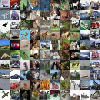
Fig. 8. Top: Precision filters (matrix C) of size 16x16 pixels learned
on color image patches of the same size. Matrix P was initialized with natural images that were taken from ImageNet [54]13 . The
a local connectivity inducing a two dimensional topographic map. model was trained using 8x8 filters divided into four sets
This makes nearby filters in the map learn similar features. Bottom with different spatial phases. Each set tiles the image with
left: Random subset of mean filters (matrix W ). Bottom right (from
top to bottom): independent samples drawn from the training data, a diagonal offset of two pixels from the previous set. Each
mPoT, GRBM and PoT. set consists of 64 covariance filters and 16 mean filters.
Parameters were learned using the algorithm described in
TABLE 1 sec. 3, but setting P to identity.
Log-probability estimates of test natural images x, and exact The first two rows of fig. 9 compare samples drawn
log-probability ratios between the same test images x and random from PoT with samples drawn from mPoT and show that
images n. the latter ones exhibit strong structure with smooth regions
separated by sharp edges while the former ones lack any
Model log p(x) log p(x)/p(n)
MoG -85 68
sort of long range structure. Yet, mPoT samples still look
GRBM FPCD -152 -3 rather artificial because the structure is fairly primitive and
PoT FPCD -101 65 repetitive. We then made the model deeper by adding two
mPoT CD -109 82
mPoT PCD -92 98 layers on the top of mPoT.
mPoT FPCD -94 102 All layers are trained by using FPCD but, as training pro-
ceeds, the number of Markov chain steps between weight
updates is increased from 1 to 100 at the topmost layer
mean filter resembling a similar Gabor specifies the initial in order to obtain a better approximation to the maximum
intensity values before the interpolation. likelihood gradient. The second hidden layer has filters of
The most intuitive way to test a generative model is to size 3x3 that also tile the image with a diagonal offset of
draw samples from it [49]. After training, we then run HMC one. There are 512 filters in each set. Finally, the third
for a very long time starting from a random image. The layer has filters of size 2x2 and it uses a diagonal offset
bottom right part of Fig. 8 shows that mPoT is actually of one; there are 2048 filters in each set. Every layer
able to generate samples that look much more like natural performs spatial subsampling by a factor equal to the size
images than samples generated by a PoT model, which of the filters used. This is compensated by an increase in
only models the pair-wise dependencies between pixels or a the number of channels which take contributions from the
GRBM model, which only models the mean intensities. The
mPoT model succeeds in generating noisy texture patches, 12. The log probability ratio is exact since the intractable partition
function cancels out. This quantity is equal to the difference of energies.
smooth patches, and patches with long elongated structures 13. Categories are: tree, dog, cat, vessel, office furniture, floor lamp,
that cover the whole image. desk, room, building, tower, bridge, fabric, shore, beach and crater.JOURNAL OF PAMI, VOL. ?, NO. ?, JANUARY 20?? 11
TABLE 2
Denoising performance using σ = 20 (PSNR=22.1dB).
Barb. Boats Fgpt. House Lena Peprs.
mPoT 28.0 30.0 27.6 32.2 31.9 30.7
mPoT+A 29.2 30.2 28.4 32.4 32.0 30.7
mPoT+A+NLM 30.7 30.4 28.6 32.9 32.4 31.0
FoE [11] 28.3 29.8 - 32.3 31.9 30.6
NLM [55] 30.5 29.8 27.8 32.4 32.0 30.3
GSM [56] 30.3 30.4 28.6 32.4 32.7 30.3
BM3D [57] 31.8 30.9 - 33.8 33.1 31.3
LSSC [58] 31.6 30.9 28.8 34.2 32.9 31.4
6.2 Denoising
The most commonly used task to quantitatively validate
a generative model of natural images is image denoising,
assuming homogeneous additive Gaussian noise of known
variance [10], [11], [37], [58], [12]. We restore images
by maximum a-posteriori (MAP) estimation. In the log
domain, this amounts to solving the following optimization
problem: arg minx λ||y − x||2 + F(x; θ), where y is the
observed noisy image, F(x; θ) is the mPoT energy function
(see eq. 12), λ is an hyper-parameter which is inversely
proportional to the noise variance and x is an estimate of
the clean image. In our experiments, the optimization is
performed by gradient descent.
For images with repetitive texture, generic prior models
usually offer only modest denoising performance compared
Fig. 9. Top row: Three representative samples generated by PoT to non-parametric models [45], such as non-local means
after training on an unconstrained distribution of high-resolution gray- (NLM) [55] and BM3D [57] which exploit “image self-
scale natural images. Second row: Representative samples gener- similarity” in order to denoise. The key idea is to compute
ated by mPoT. Third row: Samples generated by a DBN with three
hidden layers, whose first hidden layer is the gated MRF used for the a weighted average of all the patches within the test
second row. Bottom row: as in the third row, but samples (scanned image that are similar to the patch that surrounds the
from left to right) are taken at intervals of 50,000 iterations from pixel whose value is being estimated, and the current state-
the same Markov chain. All samples have approximate resolution
of 300x300 pixels. of-the-art method for image denoising [58] adapts sparse
coding to take that weighted average into account. Here,
we adapt the generic prior learned by mPoT in two simple
ways: 1) first we adapt the parameters to the denoised
filters that are applied with a different offset, see fig. 7. test image (mPoT+A) and 2) we add to the denoising
This implies that at the top hidden layer each latent variable loss an extra quadratic term pulling the estimate close to
receives input from a very large patch in the input image. the denoising result of the non-local means algorithm [55]
With this choice of filter sizes and strides, each unit at the (mPoT+A+NLM). The first approach is inspired by a large
topmost layer affects a patch of size 70x70 pixels. Nearby body of literature on sparse coding [59], [58] and consists
units in the top layer represent very large (overlapping) of a) using the parameters learned on a generic dataset of
spatial neighborhoods in the input image. natural images to denoise the test image and b) further
After training, we generate from the model by perform- adapting the parameters of the model using only the test
ing 100,000 steps of blocked Gibbs sampling in the topmost image denoised at the previous step. The second approach
RBM (using eq. 15 and 16) and then projecting the samples simply consists of adding an additional quadratic term
down to image space as described in sec. 4. Representative to the function subject to minimization, which becomes
samples are shown in the third row of fig. 9. The extra λ||y − x||2 + F(x; θ) + γ||xN LM − x||2 , where xN LM
hidden layers do indeed make the samples look more is the solution of NLM algorithm.
“natural”: not only are there smooth regions and fairly sharp Table 2 summarizes the results of these methods compar-
boundaries, but also there is a generally increased variety of ing them to the current state-of-the-art methods on widely
structures that can cover a large extent of the image. These used benchmark images at an intermediate level of noise.
are among the most realistic samples drawn from models At lower noise levels the difference between these methods
trained on an unconstrained distribution of high-resolution becomes negligible while at higher noise levels parametric
natural images. Finally, the last row of fig. 9 shows the methods start outperforming non-parametric ones.
evolution of the sampler. Typically, Markov chains slowly First, we observe that adapting the parameters and taking
and smoothly evolve morphing one structure into another. into account image self-similarity improves performanceYou can also read