Modelling the Evolution of COVID-19 in High-Incidence European Countries and Regions: Estimated Number of Infections and Impact of Past and Future ...
←
→
Page content transcription
If your browser does not render page correctly, please read the page content below
Journal of
           Clinical Medicine

Article
Modelling the Evolution of COVID-19 in
High-Incidence European Countries and Regions:
Estimated Number of Infections and Impact of Past
and Future Intervention Measures
Juan Fernández-Recio
 Instituto de Ciencias de la Vid y del Vino (ICVV), CSIC-Universidad de La Rioja-Gobierno de La Rioja,
 Ctra. Burgos Km 6, 26007 Logroño, Spain; juan.fernandezrecio@icvv.es; Tel.: +34-941-894980

 Received: 18 May 2020; Accepted: 8 June 2020; Published: 11 June 2020

 Abstract: A previously developed mechanistic model of COVID-19 transmission has been adapted
 and applied here to study the evolution of the disease and the effect of intervention measures in some
 European countries and territories where the disease has had a major impact. A clear impact of the
 major intervention measures on the reproduction number (Rt ) has been found in all studied countries
 and territories, as already suggested by the drop in the number of deaths over time. Interestingly,
 the impact of such major intervention measures seems to be the same in most of these countries.
 The model has also provided realistic estimates of the total number of infections, active cases and
 future outcomes. While the predictive capabilities of the model are much more uncertain before
 the peak of the outbreak, we could still reliably predict the evolution of the disease after a major
 intervention by assuming the subsequent reproduction number from the current study. A greater
 challenge is to foresee the long-term impact of softer intervention measures, but this model can
 estimate the outcome of different scenarios and help to plan changes for the implementation of control
 measures in a given country or region.

 Keywords: COVID-19; virus; epidemiology; disease transmission model; intervention measures

1. Introduction
     The ongoing pandemic expansion of the new SARS-CoV-2 virus has caused over 3,500,000
detected cases of coronavirus disease 2019 (COVID-19) and claimed over 240,000 lives worldwide
as of 5 May 2020 [1]. Since the first epidemic wave has dramatically hit a large number of countries,
we can learn from all available epidemiological data to understand the evolution of the disease in
order to better prepare the healthcare capacities for future pandemic waves. A recent model of
SARS-CoV-2 transmission based on estimates of seasonality, immunity and cross-immunity from past
virus pandemic data indicates the high risk of recurrent outbreaks in the coming years, according
to different scenarios [2]. Before the availability of effective vaccines and pharmaceutical treatments,
the transmission of the disease can only be controlled by prevention measures, like personal hygiene
habits, social distancing, case detection and isolation, or by contact tracing. Strict social distancing
enforced by the authorities has been the strategy of choice by the majority of countries in this first
epidemic outbreak, implemented as different measures in each country (imposing or encouraging home
confinement, closing schools and workplaces and banning assemblies and gatherings, among others).
Given that this usually involves a strong economic and behavioral impact in a society, it is urgently
necessary to understand the evolution of the disease in each country or territory and to estimate the
effect of implementing such control measures. A major problem is that in most countries, only a small
portion of the infected individuals is detected, and as a consequence, undetected contagious patients

J. Clin. Med. 2020, 9, 1825; doi:10.3390/jcm9061825                                  www.mdpi.com/journal/jcm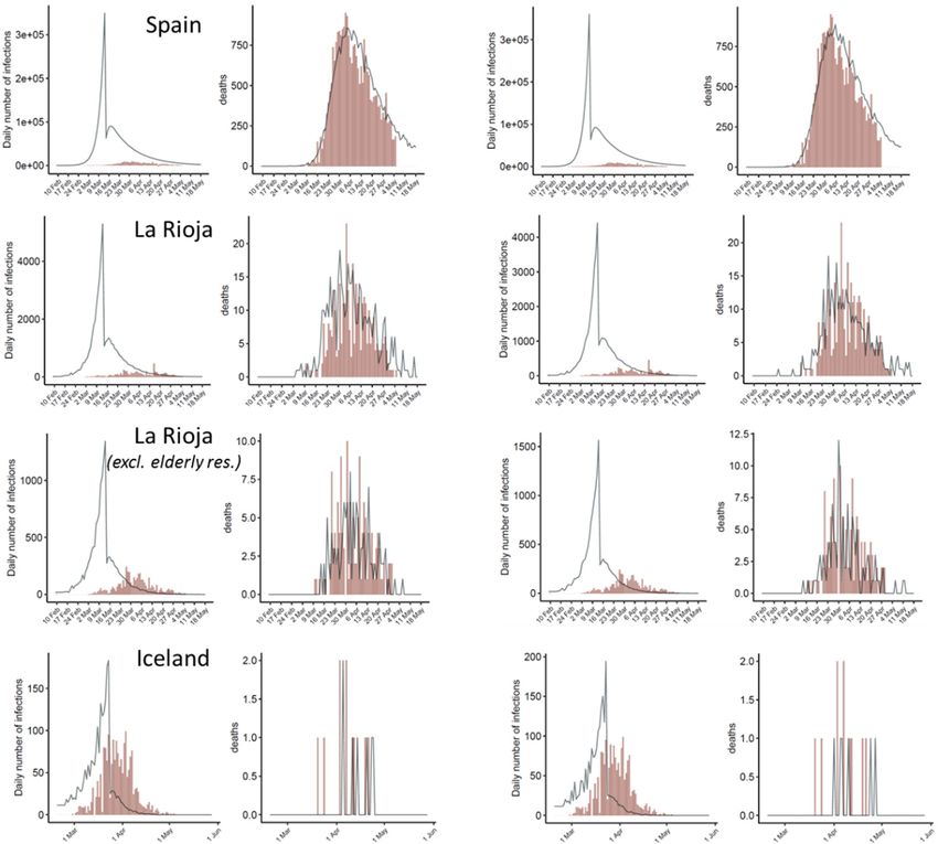
J. Clin. Med. 2020, 9, 1825                                                                         2 of 17

are the major cause of the expansion of the disease, which is the main limitation in foreseeing the effect
of intervention measures. In the absence of large-scale detection tests able to be applied to an entire
country population, mathematical modeling can help to estimate the dynamics of infections based on
available epidemiological data. Indeed, a recent networked dynamic metapopulation model using
Bayesian inference and based on reported infections and mobility data suggests a high proportion of
undocumented infections in the first SARS-CoV-2 outbreak in China [3]. That model compared the
initial transmission dynamics with those after greater control measures were introduced, showing a
clear reduction in the transmission rate and the effective reproduction number. However, the specific
impact of the different control measures was difficult to analyze at that time.
      In this context, a Bayesian mechanistic model was recently proposed to estimate the effects of
specific intervention measures on the reproduction number in 11 countries by inferring the number of
infections from the observed deaths over time [4], assuming an infection fatality ratio (IFR) that was
different for each country, adjusted to the age distribution of their population. A major assumption of
that study was that the intervention measures had the same relative effect in all countries, which is not
necessary true. For instance, according to large-scale mobile phone data [5], the effect of lockdown
measures on the mobility of the population was clearly different in each country. The level of isolation
of transmitting cases not only depends on the intervention to the general population, but also on the
percentage of detected patients, which might make the isolation of such patients more or less effective.
      Another limitation of the mentioned study [4] is that, at that moment, the pandemic was in the
early stages of its evolution. Since the peak of the outbreak had not yet been reached in the studied
countries, the impact of intervention could be followed based solely on small changes in the slope of
the growth of reported deaths over time, with a large degree of uncertainty. Moreover, for some of the
intervention measures, an insufficient time had passed to see a real impact on the number of deaths.
As a consequence, the impact of the intervention measures of most of the countries were probably
underestimated, and the forecast anticipated a larger number of expected infections and deaths than
those found in the following weeks.
      Here, a new study has been performed by using current data on the five European countries with
the highest number of total cases (Spain, Italy, UK, France and Germany), in which the disease has
significantly evolved and seems to have overpassed the outbreak peak. In this work, the analysis
has also included Iceland and the Spanish region of La Rioja, with comparable populations, in which
the number of reported cases in proportion to their population is among the highest ones in Europe.
The model has been adapted by fitting it individually to each country, and by simplifying the number
of intervention measures to evaluate. The result is a model that nicely explains the evolution of
the disease and that can describe the effective impact of the intervention measures and estimate the
outcome of future interventions.

2. Methods

2.1. Data Collection
     Daily real-time death data was gathered from the ECDC (European Centre of Disease Control).
Table 1 shows the up-to-date (5 May 2020) detected cases and reported deaths for high-incidence
countries (Spain, Italy, United Kingdom, Germany, France, Iceland), as well as for La Rioja, the region
in Spain with the highest number of incidences relative to its population. In the latter, the model is
also applied to the data after excluding the population from elderly retirement homes with reported
cases. The high incidence of cases in elderly retirement homes in European countries suggests that
transmission of the disease has followed different patterns in these cases, and the impact of general
lockdown measures might not be the same as in the general population. Since this data is available for
this work only in the case of La Rioja, it has been considered worthy of inclusion in the analysis.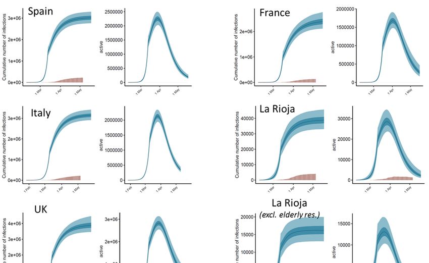
J.J. Clin.
Clin. Med. 2020, 9,
Med. 2020, 9, 1825
x FOR PEER REVIEW 33 of
of 17
16
Table 1. Reported COVID-19 cases per country/region (updated 5 May 2020).
Table 1. Reported COVID-19 cases per country/region (updated 5 May 2020).
Country/Region Total Detected Cases Cases per 100 k People Total Reported Deaths
Country/Region Total Detected Cases Cases per 100 k People Total Reported Deaths
Spain 219,329 469 25,613
Spain 219,329 469 25,613
Italy 211,938 351 29,079
Italy 211,938 351 29,079
UK UK 190,584
190,584 287
287 28,734
28,734
Germany
Germany 163,860
163,860 198
198 68316831
France
France 131,863
131,863 197
197 25,201
25,201
La Rioja
La Rioja (Spain)
(Spain) 3969
3969 1256
1256 336336
La Rioja (Spain) 1 2988 952 143
La Rioja (Spain) 1 2988 952 143
Iceland 1799 509 10
1
Iceland 1799 509 10
Excluding data from elderly retirement homes with reported cases. Reported deaths (excluding those in elderly
1 Excluding data from elderly retirement homes with reported cases. Reported deaths (excluding
retirement homes) correspond to 5 May 2020, but detected cases outside elderly retirement homes have been
extrapolated from data
those in elderly on 15 May
retirement 2020. correspond to 5 May 2020, but detected cases outside elderly
homes)
retirement homes have been extrapolated from data on 15 May 2020.
2.2. Estimating New Infections and Deaths over Time
2.2. Estimating New Infections and Deaths over Time
The major details of the model have been described elsewhere [4]. Basically, the expected number
The D
of deaths major detailsday
i in a given of ithe
is amodel
functionhave been
of the numberdescribed elsewhere
of infections [4]. Basically,
Ij occurring j=1
the expected
in the previous
.number
. . i−1 days,
of deaths Di intoaa given
according day icalculated
previously is a function of the number(ITD)
infection-to-death of infections Ij occurring
probability inand
distribution the
previous
an j = 1…i−1
estimated days,
infection according
fatality to afor
ratio (IFR) previously
each country calculated infection-to-death
(Equation (1)). (ITD) probability
distribution and an estimated infection fatality ratio (IFR) for each country (Equation (1)).
Xi−1
Di = I j ·IFR·ITDi−j (1)
= j=1 ∙ ∙ (1)
The
The infection-to-death
infection-to-death (ITD)
(ITD) probability
probability distribution
distribution waswas modelled,
modelled, using
using previous
previous
epidemiological
epidemiological data from the early outbreak in China [6,7], by adding up two distributions:
data from the early outbreak in China [6,7], by adding up two independent independent
(i) the infection-to-onset
distributions: (incubation period)
(i) the infection-to-onset distribution,
(incubation estimated
period) as a Gamma
distribution, probability
estimated density
as a Gamma
function with mean 5.1 days and a coefficient of variation 0.86; and (ii) the onset-to-death (time
probability density function with mean 5.1 days and a coefficient of variation 0.86; and (ii) the onset- between
onset
to-deathand(time
death) distribution,
between estimated
onset and death)asdistribution,
a Gamma probability
estimated as density function
a Gamma with a mean
probability of
density
18.8 days with
function and aa coefficient
mean of 18.8of variation
days and 0.45 [4]. The of
a coefficient resulting ITD
variation probability
0.45 distribution
[4]. The resulting ITDisprobability
shown in
Figure 1b.
distribution is shown in Figure 1b.
Figure
Figure 1.1. Probability
Probability distributions
distributions used
used in
in this
this work
work for
for (a)
(a) serial
serial interval,
interval, (b)
(b) infection-to-death
infection-to-death and
and
(c) infection-to-recovery.
(c) infection-to-recovery.
The infection fatality ratio (IFR) is the probability of death for an infected case. The values
The infection fatality ratio (IFR) is the probability of death for an infected case. The values used
used here for COVID-19 are derived from previous estimates [8] and are calculated for each country
here for COVID-19 are derived from previous estimates [8] and are calculated for each country
according to the age-distribution population [6,7]. For La Rioja, the same IFR is used as for Spain.
according to the age-distribution population [6,7]. For La Rioja, the same IFR is used as for Spain. For
For Iceland, the general IFR value of 0.657% was initially used, as previously reported by combining
Iceland, the general IFR value of 0.657% was initially used, as previously reported by combining
estimates of case fatality ratios with information on infection prevalence in China [7]. This IFR estimate
estimates of case fatality ratios with information on infection prevalence in China [7]. This IFR
provided an expected number of infected and active cases close to the detected ones. However, the case
estimate provided an expected number of infected and active cases close to the detected ones.
However, the case fatality rate (CFR), an empirical value obtained from the number of deaths over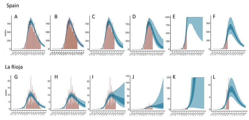
J. Clin. Med. 2020, 9, 1825                                                                                 4 of 17

fatality rate (CFR), an empirical value obtained from the number of deaths over the detected cases,
gives a value of CFR = 0.556% for Iceland, and the true IFR could be even smaller [9], so this CFR
value (0.556%) was finally used as a better estimate of IFR in Iceland. The IFR values used here for the
different countries are shown in Table 2.

                      Table 2. Model parameters (intervention dates and IFR) used in this work.

     Country/Region           Time of Intervention     Days from First 100 Cases to Intervention Time    IFR
           Spain                   14 March                                         11                  0.926%
            Italy                  11 March                                         16                  1.090%
             UK                    24 March                                         18                  0.919%
         Germany                   22 March                                         20                  1.093%
          France                   17 March                                         15                  1.153%
         La Rioja                  14 March                                          5                  0.926%
          Iceland                  24 March                                          8                  0.556%

     In this model, the expected number of new infections Ij occurring in a given day j is a function
of the number of infections Ik in the previous k = 1 . . . j−1 days, according to a serial interval (SI)
distribution, and the reproduction number (Rt ) (Equation (2)).

                                                            j−1
                                                            X
                                                     Ij =          Ik ·Rt ·SI j−k                                (2)
                                                            k =1

     The SI probability distribution was modelled as a Gamma probability density function with a
mean of 6.5 days and a coefficient of variation 0.62 (Equation (2)), as previously described [4], and is
shown in Figure 1a. The reproduction number (Rt ) had an initial constant value R0 (a parameter
that was left to optimize during the fitting of the model independently for each country), and was
assumed to change after an intervention to another value which was kept constant over time until a
new intervention (the new Rt value after a given intervention is also a parameter to optimize during the
model fitting). For simplicity, the entire population was assumed to be susceptible to infection during
model fitting, but for long-term predictions based on the resulting model parameters (see Section 3.5),
the infected cases were assumed to be protected from further infection.

2.3. Model Fitting
      The expected number of deaths obtained from the above described model (Equations (1) and
(2)) were fitted to the observed number of daily deaths, and were assumed to follow a negative
binomial distribution, as previously described [4]. In the case of Iceland, both the observed number
of daily deaths and the cumulative number of observed deaths were fitted, because the observed
daily deaths alone did not provide reliable fitting due to the small size of the sample. Following the
initial procedure [4], the model included only observed deaths from the day after a given country
had cumulatively observed over 10 deaths (d10 ), given that the early stages of the epidemic in a given
country might be dominated by infections that are not local. An exception was made in the case
of small regions or countries with a low number of deaths, such as Iceland and La Rioja, in which
observed deaths were included from the day of the first death (d1 ). Similarly, according to the original
procedure [4], the initial infections of the model were assumed to be 30 days before this d10 (or d1 ) day,
starting with 6 consecutive days with the same number of infections, which was left as a parameter
to be optimized in the fitting procedure. The initial infections for the first 6 days and the R0 and
Rt values after each intervention were defined as parameters to optimize in the model. Fitting was
done in the probabilistic programming language Stan, using an adaptive Hamiltonian Monte Carlo
(HMC) sampler. Eight chains for 4000 iterations, with 2000 iterations of warmup and a thinning
factor 4 were run. Running of 200 sampling iterations with 100 warmup iterations yielded very
similar results in most of the cases, suggesting that convergence was achieved early in the fitting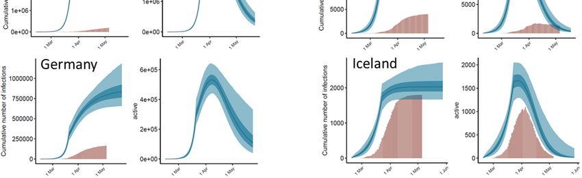
J. Clin. Med. 2020, 9, 1825 5 of 17
process. See more details in the original description of the model [4]. The original code is available at
J. Clin. Med. 2020, 9, x FOR PEER REVIEW 5 of 16
https://github.com/ImperialCollegeLondon/covid19model/releases/tag/v1.0.
In the original
process. See morestudy,details parameters
in the originalwere estimated
description of the simultaneously for 11
model [4]. The original countries,
code but
is available at here
the model was fitted to the data from each country/region
https://github.com/ImperialCollegeLondon/covid19model/releases/tag/v1.0. independently, since the effect of each
intervention on R
In the original
t is notstudy, parameters were estimated simultaneously for 11 countries, but here the of
necessarily the same in all areas. To simplify the model, here the number
interventions
model was were reduced,
fitted to the and
datathe possibility
from of having anindependently,
each country/region end date for any intervention
since the effect ofwaseachadded.
intervention
The inclusion on Rtone
of only is not necessarily was
intervention the same
foundin to
all be
areas. To simplify
sufficient the model,
to explain here while
the data, the number of
the addition
interventions
of further were reduced,
intervention steps didand thesignificantly
not possibility of improve
having antheendfitting.
date for any intervention was added.
The inclusion of only one intervention was found to be sufficient to explain the data, while the
addition of
2.4. Predictive further
Model intervention
from steps
a Given Set did not significantly improve the fitting.
of Parameters
The use of continuous
2.4. Predictive Model from serial
a Giveninterval and infection-to-death probability distributions to estimate
Set of Parameters
the number of deaths from the new infections is needed for the efficiency of the fitting procedure, but in
The use of continuous serial interval and infection-to-death probability distributions to estimate
reality,
thethe deaths
number ofderived from
deaths from thethe
newnewly infected
infections people
is needed foron
thea efficiency
given dayofwill be distributed
the fitting procedure,inbut
specific
days in
in reality,
a discrete manner. The overall discrete distributions will expectedly follow
the deaths derived from the newly infected people on a given day will be distributed in the serial interval
and infection-to-death probability
specific days in a discrete manner. distributions, but the distributions
The overall discrete number of deaths for each set
will expectedly of infections
follow the serial will
happen in a single
interval discrete distribution,
and infection-to-death which
probability will be different
distributions, but the each
number time, especially
of deaths if the
for each setnumber
of
infections will happen in a single discrete distribution, which will be different
of infections is small. In Figure 2 we can compare some random discrete distributions for expected each time, especially
deathsif the number
over time of forinfections
samplesisof small. In Figure
different 2 we
sizes = 1,compare
(n can 10, 100, some random
1000) discrete
according todistributions
the continuous
infection-to-death probability distributions used here vs. several discrete samples derivedtofrom
for expected deaths over time for samples of different sizes (n = 1, 10, 100, 1000) according the the
continuous infection-to-death probability distributions used here vs. several discrete samples derived
same infection-to-death distribution. As the sample size (n) increases, the discrete and continuous
from the same infection-to-death distribution. As the sample size (n) increases, the discrete and
distributions tend to converge, but for small size samples, assuming continuous distribution might not
continuous distributions tend to converge, but for small size samples, assuming continuous
represent a givenmight
distribution instance.
not represent a given instance.
Figure 2. Examples
Figure 2. Examplesof random
of random discrete
discretedistributions
distributions of samplesofofn n
of samples = 10,
= 1, 1, 10,
100,100,
10001000 expected
expected deaths,
deaths,
according
according to the infection-to-death (ITD) probability distribution used in this work. For samples of a of
to the infection-to-death (ITD) probability distribution used in this work. For samples
a small size,
small size,the
thedistribution canbebe
distribution can very
very different
different fromfrom the probability
the probability curveinshown
curve shown in while
Figure 1b, Figure 1b,
whilefor
forsamples
samplesofofa alarger
larger size
size (e.g.,
(e.g., 100100
or or 1000
1000 deaths),
deaths), thethe discrete
discrete distributions
distributions get closer
get closer to theto the
probability
probability distribution
distribution curve.
curve.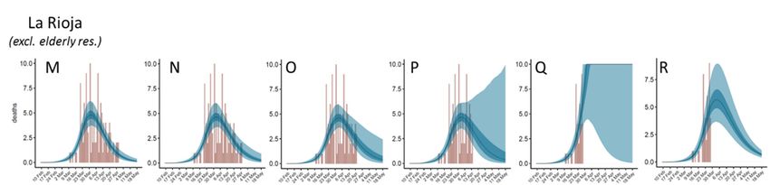
J. Clin. Med. 2020, 9, 1825                                                                         6 of 17

     Therefore, for a better visual comparison between the predictive results of our model and the
set of reported deaths over time (discrete distribution), it is possible to generate instances of discrete
distributions over time of the expected number of new infections and deaths computed with the
parameters obtained during the fitting procedure (usually, from a set of parameters randomly selected
among the ones obtained). These instances can be generated by randomly assigning every case (from
the set of new infections or deaths to be distributed) to a specific day according to the serial interval
and infection-to-death probability distributions.

2.5. Estimating Active Cases from Model Predictions
     Basically, the expected number of recovered cases RECOVi in a given day i is a function of the
number of the estimated new infections Ij occurring in the previous j = 1 . . . i−1 days, according
to a previously calculated infection-to-recovery (ITR) probability distribution, after discounting the
percentage of new infected cases with outcome of death from infection fatality ratio (IFR) (Equation (3)).

                                               i−1
                                               X
                                   RECOVi =           I j ·(1 − IFR)·ITRi− j                           (3)
                                                j=1

     The infection-to-recovery (ITR) probability distribution was modelled by adding up two
independent distributions: (i) the infection-to-onset (incubation period) distribution, estimated
as a Gamma probability density function with mean 5.1 days and a coefficient of variation 0.86; and (ii)
the onset-to-recovery (time between onset and recovery) distribution, estimated as a Gamma probability
density function with a mean of 24.7 days and a coefficient of variation 0.35 [7]. The resulting ITR
probability distribution is shown in Figure 1c. The estimated active cases for a given day is calculated
by subtracting the estimated cumulative number of recovered cases from the estimated cumulative
number of cases for that day.

3. Results

3.1. Model Suggests a Significant Impact of Intervention Measures on Disease Transmission
     The model was fitted (see Methods) to data from the countries with the highest number of reported
cases in the EU/EEA and the UK as of 5 May 2020 (Spain, Italy, United Kingdom, Germany and France)
(Table 1). They are actually the countries with the largest population. For comparison, the data for small
countries and regions are also added, such as Iceland, and the Spanish region La Rioja, which have
a comparable population (over 300,000 inhabitants) and show a high incidence of cases per 100,000
people. Actually, La Rioja is the region with highest number of detected cases relative to its population
in Spain and probably in Europe. For comparison, the region in the United States with the highest
level of incidence is New York City, in boroughs like The Bronx with 2667 detected cases per 100,000 as
of 5 May 2020 [10].
     The study here focuses on the effect of the single most relevant intervention measure implemented
by authorities (defined as “lockdown ordered” in a previous study [4]). For La Rioja, the same
lockdown date was used as for Spain (14 March). For Iceland, the date of 24 March has been considered,
when a nation-wide ban was enforced on public assemblies over 20, as well as the closure of bars
and most public businesses. The dates of these interventions are shown in Table 2. After fitting the
model for each country/region independently, the estimated number of daily infections and deaths
derived from the model are shown in Figure 3, in comparison with the reported ones. The resulting
reproduction number values derived from the model provide an estimation of the impact of the
intervention measures on the transmission dynamics of the disease in each country (Table 3).
     We can observe that the final Rt after major intervention is similar in all analyzed countries
(except in Iceland and in La Rioja when elderly residences with reported cases were excluded),
with mean values ranging from 0.57 (La Rioja region) to 0.71 (Germany), and an averaged value of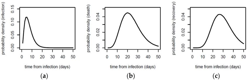
J. Clin. Med. 2020, 9, 1825 7 of 17
0.625. Interestingly, a recent calculation on the reproduction number (R) in Germany, estimated from
a nowcasting approach on reported COVID-19 cases with illness onset up to three days before data
closure, provides a current estimate of R = 0.71 (95% prediction interval: 0.59–0.82) [11], which is
virtually the same as the one calculated here with the disease transmission model based on the reported
deaths. Regarding the relative values of Rt after intervention (in percentage relative to R0 before
intervention), they ranged from 12.0% (Spain) to 20.7% (Italy). These values seem to depend not only
on the effectiveness of the intervention measures, but also on the evolution of the disease prior to
intervention, described by R0 , which seems to be different in each country (Table 3). As a warning note,
this effect in relative terms was the one assumed to be constant for the same type of intervention in the
different countries in the original application of the model [4], an assumption that does not seem to
be valid.
J. Clin. Med. 2020, 9, x FOR PEER REVIEW 7 of 16
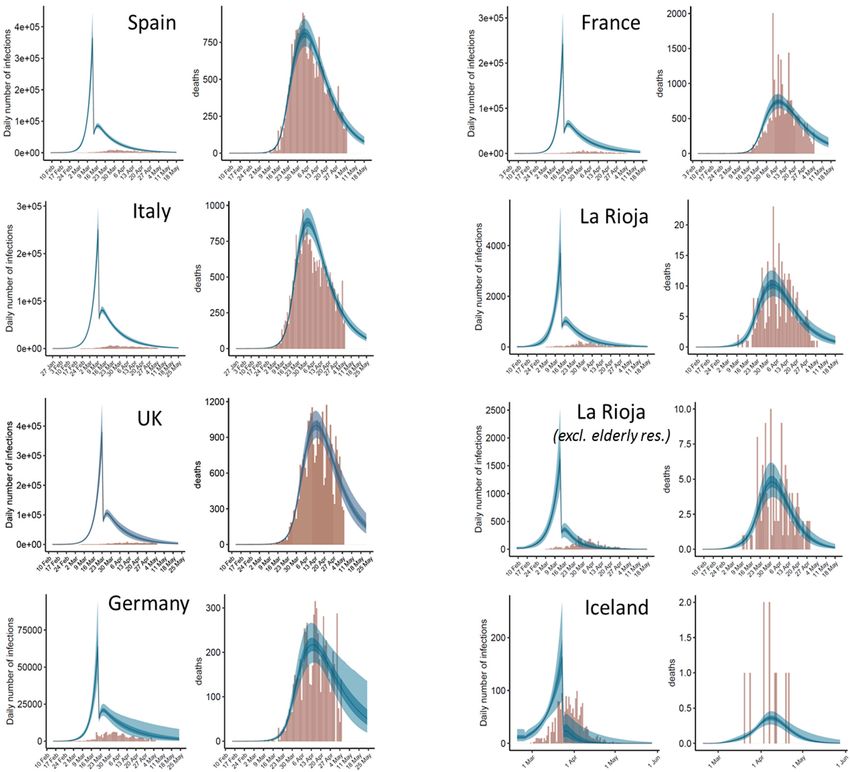
Figure 3.
Figure 3. Estimates
Estimatesof ofinfections
infectionsand
anddeaths
deathsoverovertime
timeafter
afterindependent
independent application
application of of
thethe
model
modelto
each country and region. For each country, the left plot shows the predicted
to each country and region. For each country, the left plot shows the predicted daily infections as daily infections as
compared with
compared with the reported ones,
the reported ones, and
and the
the right
right plot
plot shows
shows thethe expected
expected daily
daily deaths
deaths asas compared
compared
with the
with the observed
observedones.
ones.Expected
Expected values
valuesareare
shown
shownas blue bands:
as blue lightlight
bands: blueblue
(95%(95%
CI), dark blue (50%
CI), dark blue
CI) and line (median). Observed values are shown as brown bars. The estimates
(50% CI) and line (median). Observed values are shown as brown bars. The estimates of Rt before of R t before and after
intervention
and resulting resulting
after intervention from thefrom
modeltheare the ones
model in ones
are the Tablein3.Table
In all3. cases, after intervention,
In all cases, Rt is
after intervention,
significantly reduced to a value well below 1 and the number of new infections decreases.
Rt is significantly reduced to a value well below 1 and the number of new infections decreases. In the In the La
Rioja
La second
Rioja panel,
second daily
panel, observed
daily deaths
observed do not
deaths include
do not those
include fromfrom
those elderly retirement
elderly homes,
retirement but
homes,
daily reported cases are the total ones, since the daily reported cases outside elderly
but daily reported cases are the total ones, since the daily reported cases outside elderly residences was residences was
not available
not available for
for this
this work.
work.
Table 3. Estimated reproduction numbers (before and after intervention) and initial number of
infections resulting from the model (shown mean values, with 95% credible interval).
Estimated Infections in
Country/Region Ro Rt after Intervention
First 6 Days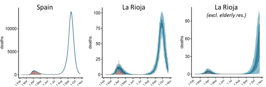
J. Clin. Med. 2020, 9, 1825                                                                                         8 of 17

      Table 3. Estimated reproduction numbers (before and after intervention) and initial number of infections
      resulting from the model (shown mean values, with 95% credible interval).

      Country/Region                    R0            Rt after Intervention      Estimated Infections in First 6 Days
             Spain                4.82 (4.18–5.51)       0.58 (0.52–0.65)                     396 (153–819)
              Italy               3.14 (2.93–3.38)       0.65 (0.60–0.70)                     623 (370–964)
               UK                 3.60 (3.26–3.95)       0.60 (0.50–0.70)                    749 (396–1276)
           Germany                3.68 (2.91–4.57)       0.71 (0.54–0.89)                     314 (70–876)
             France               4.47 (3.93–5.06)       0.64 (0.55–0.74)                      113 (43–242)
            La Rioja              3.29 (2.41–4.48)       0.57 (0.45–0.70)                        72 (8–239)
           La Rioja 1             2.55 (2.06–3.34)       0.41 (0.21–0.59)                      123 (27–279)
            Iceland               1.84 (1.37–2.38)       0.26 (0.01–0.69)                       75 (24–162)
                              1   Excluding data from elderly retirement homes with reported cases.

     The model has also been applied by including additional interventions, such as the work lockdown
period ordered in Spain and La Rioja region between 1 and 6 April 2020 (see Supplementary Materials
Table S1), or the contention period around 7 March 2020 in La Rioja after a very localized outbreak
in the city of Haro (data not shown), but no significant improvement of the model was found
(Supplementary Materials Figure S1). The effect of an additional indirect intervention in Iceland
was also modelled (on 3 April, a recently released mobile app to trace infections had almost 75,000
downloads, which might have had an impact on the reproduction number), with no significant changes
(Supplementary Materials Table S1, Supplementary Materials Figure S1). In general, one would expect
that a series of stepwise interventions will have a smoother effect on the reproduction number (and
therefore on the number of new infections) than just a single strict intervention. One could also
speculate whether other early measures taken in some countries have contributed to a decrease in
their initial R0 values or to a delay in the initial number of infections at the early stage of the epidemic
outbreak, but this is beyond this study.
     It is interesting to analyze the results after applying the model to La Rioja data after excluding data
in elderly retirement homes with reported cases (Figure 3, Table 3). As expected, the propagation of the
disease in the elderly retirement homes and in the general population is very different. Outside these
elderly retirement homes, the propagation rates decrease before and after intervention. It would be
interesting to know whether the same effect can be seen in other countries.

3.2. Estimated Number of Total Infections and Active Cases
     From the values obtained by the model, we can estimate the daily cumulative number of infections.
The evolution of the predicted cumulative number of infections in comparison with the detected cases
over time can be seen in Figure 4, with the detailed data per country as of 5 May 2020 in Table 4.
The highest detection rates (that is, total detected cases with respect to the total predicted ones) are
found in Germany (21%) and Iceland (54%). These are actually countries with a high number of tests
performed relative to their population. In Germany, there were a reported 30.4 tests per thousand
people as of 22 April 2020 [12], one of the highest rates in Europe. In Iceland there were a reported
151.2 tests per thousand people as of 5 May 2020, the highest rate in Europe [13]. In other territories,
the total number of predicted cases is much higher than the reported ones, with detection rates that
range from 5% (UK) to 10% (La Rioja). Interestingly, the detection rate in La Rioja is better than in
Spain (7%). Moreover, when data from elderly retirement homes with reported cases are excluded,
the detection rate in the rest of the population in La Rioja is much larger (18%). This is consistent
with the fact that La Rioja was the Spanish region with the highest number of PCR tests per thousand
people (56.9, as of 27 April 2020; as compared to 22.0 in Spain) [14].
     From the model results, we can also estimate the number of daily active cases per country
(Figure 4). For comparison, the reported number of active cases in La Rioja [15] and in Iceland [13] are
shown. In La Rioja, there were a reported 1257 active cases as of 5 May 2020. As indicated in Table 4,
the model estimated a median value of 4746 for the same date (95% CI: 2821–8088), which indicates a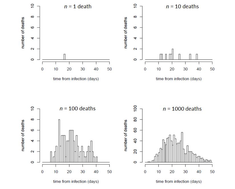
J. Clin. Med. 2020, 9, 1825                                                                                                       9 of 17

detection rate of 27%. When data from elderly retirement homes were excluded, the model estimated a
median value of 945 active cases (95% CI: 464–2059). Considering that the reported 1257 active case
as of 5 May include cases from elderly residences (e.g., 112 out of the 741 active cases as of 15 May
were from elderly retirement homes [15]), this indicates a detection rate of active cases close to 100%.
In Iceland, there were a reported 32 active cases as of 5 May 2020, while our model predicted a median
value of 141 active cases for the same date (95% CI: 78–605) (Table 4), indicating a detection rate of 23%
(which is lower than the general detection rate for the total cumulative cases).
J. Clin. Med. 2020, 9, x FOR PEER REVIEW                                                                                           9 of 16

       Figure4.4. Estimated
      Figure       Estimated cumulative
                                 cumulative infections
                                                infections and
                                                             and active
                                                                   active cases
                                                                            cases from
                                                                                   from an an independent
                                                                                                independent application
                                                                                                               application ofof the
                                                                                                                                 the
       model   to  each   country    and   region.   For each   country,    the  left  plot   shows
      model to each country and region. For each country, the left plot shows the estimated cumulativethe  estimated   cumulative
       infectionsfor
      infections    foreach
                        eachdaydayasas   compared
                                      compared        with
                                                   with the the  reported
                                                             reported    ones,ones,  andright
                                                                               and the       the right  plot shows
                                                                                                 plot shows          the expected
                                                                                                              the expected   active
       active  cases  for  each   day   (in  some   countries,  they   are   compared      with   the  reported
      cases for each day (in some countries, they are compared with the reported ones). Expected values are      ones).  Expected
       values as
      shown    areblue
                    shown    as blue
                         bands:   lightbands:   lightCI),
                                         blue (95%     bluedark
                                                            (95%    CI),(50%
                                                                 blue     darkCI)
                                                                                blueand(50%
                                                                                          lineCI)  and lineObserved
                                                                                                (median).    (median).values
                                                                                                                         Observed
                                                                                                                                are
       values  are  shown    as  brown    bars.  The  estimates    of R t before   and   after  intervention
      shown as brown bars. The estimates of Rt before and after intervention resulting from the model          resulting  from are
                                                                                                                                 the
       model
      the  onesare
                 in the ones
                     Table  3. in
                               In Table   3. Inafter
                                   all cases,   all cases, after intervention,
                                                     intervention,                 Rt is significantly
                                                                      Rt is significantly      reduced toreduced
                                                                                                            a valuetowell
                                                                                                                      a value
                                                                                                                          belowwell1
       below
      and   the1number
                  and theofnumber        of newdecreases.
                              new infections      infections Indecreases.
                                                                  the La RiojaIn the   La Rioja
                                                                                  second     panel,second    panel,
                                                                                                     estimates       estimates
                                                                                                                are derived      are
                                                                                                                              from
       derived from
      observed    deathsobserved     deaths after
                           after excluding     thoseexcluding   those
                                                      from elderly       from elderly
                                                                      retirement    homes,retirement    homes, butinfections
                                                                                                but accumulated      accumulated
                                                                                                                               and
       infections   and   active    cases   over  time   are  the  total   ones,   since    the  daily  cases
      active cases over time are the total ones, since the daily cases excluding elderly retirement homes      excluding    elderly
                                                                                                                               was
       retirement
      not  available homes   was
                       for this     not available for this work.
                                work.

       Table 4. Estimated cumulative infections as of 5 May 2020 (shown median values with 95% credible interval).

                                Estimated Total                                                                  Estimated Active
   Country/Region                                         Detection Rate         % Population Infected
                                   Infections                                                                         Cases
        Spain                 2990K (2742K–3269K)        7.3% (6.7–8.0%)              6.4% (5.9–7.0%)           415K (329K–538K)
         Italy                3094K (2868K–3358K)        6.9% (6.3–7.4%)              5.1% (4.7–5.6%)           445K (365K–551K)
          UK                  3800K (3406K–4292K)        5.0% (4.4–5.6%)              5.6% (5.0–6.3%)           998K (739K–1369K)
       Germany                 793K (641K–1024K)        20.6% (16.0–25.6%)            0.9% (0.8–1.2%)           245K (142K–451K)
J. Clin. Med. 2020, 9, 1825 10 of 17
Table 4. Estimated cumulative infections as of 5 May 2020 (shown median values with 95%
credible interval).
Estimated Total % Population Estimated Active
Country/Region Detection Rate
Infections Infected Cases
Spain 2990K (2742K–3269K) 7.3% (6.7–8.0%) 6.4% (5.9–7.0%) 415K (329K–538K)
Italy 3094K (2868K–3358K) 6.9% (6.3–7.4%) 5.1% (4.7–5.6%) 445K (365K–551K)
UK 3800K (3406K–4292K) 5.0% (4.4–5.6%) 5.6% (5.0–6.3%) 998K (739K–1369K)
Germany 793K (641K–1024K) 20.6% (16.0–25.6%) 0.9% (0.8–1.2%) 245K (142K–451K)
France 2351K (2089K–2693K) 5.6% (4.9–6.3%) 3.6% (3.2–4.1%) 482K (341K–715K)
La Rioja 38,505 (32,850–45,155) 10.3% (8.8–12.1%) 12.2% (10.4–14.3%) 4746 (2821–8088)
La Rioja 1 16,205 (13,095–19,972) 18.4% (15.0–22.8%) 5.2% (4.2–6.4%) 945 (464–2059)
Iceland 2029 (1669–2647) 88.7% (68.0–100%) 0.6% (0.5–0.7%) 141 (78–605)
1 Excluding data from elderly retirement homes with reported cases.
3.3. Predicting Discrete Distributions of Infections and Deaths
A continuous distribution of the expected new infected cases and deaths provides a smooth
curve that is suitable for parameter optimization. However, in reality, the infections and deaths are
obviously distributed in a discrete manner. For better visualization of the predicted data, random
discrete distributions of the expected infections and deaths have been generated, according to the
continuous probability distributions based on randomly selected parameters among the ones resulting
from the model (see Section 2.4). Figure 5 shows some random discrete samples of the predicted
infections and deaths, which resemble better the noisy distribution of the reported data, especially in
small countries and regions.obviously distributed in a discrete manner. For better visualization of the predicted data, random
discrete distributions of the expected infections and deaths have been generated, according to the
continuous probability distributions based on randomly selected parameters among the ones
resulting from the model (see Section 2.4). Figure 5 shows some random discrete samples of the
predicted
J. infections
Clin. Med. 2020, 9, 1825 and deaths, which resemble better the noisy distribution of the reported11data,
of 17
especially in small countries and regions.
Figure 5. Instances of discrete distributions of the estimated number of daily infections and deaths
Figure 5. Instances of discrete distributions of the estimated number of daily infections and deaths
randomly sampled according to the serial interval and infection-to-death probability distributions,
randomly sampled according to the serial interval and infection-to-death probability distributions,
based on randomly selected sets of reproduction numbers and initial infections among the ones
based on randomly selected sets of reproduction numbers and initial infections among the ones obtained
obtained by the fitted model (black lines), as compared to the reported data (brown bars). Each row
by the fitted model (black lines), as compared to the reported data (brown bars). Each row represents a
represents a country,
country, with with two
two instances instancesdistributions.
of discrete of discrete distributions. When the
When the number number
of daily of dailyand
infections infections
deaths
is large (e.g., Spain), the predicted discrete distributions are closer to the continuous ones (Figure 3),
but when these numbers are smaller (e.g., La Rioja and Iceland), the discrete distributions resemble
better the rough distribution of reported data over time. In the La Rioja second panel, observed
deaths do not include those from elderly retirement homes, but daily reported cases are the total ones,
since daily cases excluding elderly retirement homes was not available for this work.
3.4. The Reliability of the Predictions Depends on the Stage of the Epidemic Outbreak
The credible intervals of the parameters and estimated data provided by the model help to assess
the robustness of the predictions. In the graphical plots of estimated daily cases and deaths (Figure 3),
we can visualize the predictions for a few days beyond the last day of data (5 May 2020). In general,
in countries where more time has passed since the peak of the outbreak (e.g., Spain, Italy), the variability
in the estimated data beyond the last day of data is smaller than in countries in which fewer days
have passed from the time of the peak (e.g., Germany, UK). As a validation test, in order to evaluate
the capabilities of the model to predict the evolution of the disease beyond current date, it has been
fitted again to Spain and La Rioja data (with and without elderly residences cases), after removing the
reported deaths corresponding to the last week, the last two weeks or the last three weeks of data in
Spain and La Rioja (Figure 6B–D,H–J,N–P).variability in the estimated data beyond the last day of data is smaller than in countries in which
fewer days have passed from the time of the peak (e.g., Germany, UK). As a validation test, in order
to evaluate the capabilities of the model to predict the evolution of the disease beyond current date,
it has been fitted again to Spain and La Rioja data (with and without elderly residences cases), after
removing the reported deaths corresponding to the last week, the last two weeks or the last 12
J. Clin. Med. 2020, 9, 1825
three
of 17
weeks of data in Spain and La Rioja (Figure 6B–D,H–J,N–P).
Figure
Figure 6.
6. Estimated deathsfor
Estimated deaths forSpain
Spain (upper
(upper row)
row) andand La Rioja
La Rioja (total(total
data: data:
middlemiddle row; excluding
row; excluding elderly
elderly residences:
residences: bottombottom row) derived
row) derived from thefrom the(A,G,M)
model model (A,G,M) in comparison
in comparison to the predictions
to the predictions obtained
obtained after removing
after removing the (B,H,N),
the last week last weeklast
(B,H,N),
2 weekslast 2 weeks
(C,I,O), last(C,I,O),
3 weekslast 3 weeks
of data of or
(D,J,P) data (D,J,P)data
keeping or
keeping data just up to 1 week to the peak (E,K,Q), the latter also after keeping constant
just up to 1 week to the peak (E,K,Q), the latter also after keeping constant Rt = 0.625 (F,L,R). R t = 0.625
(F,L,R).
Table 5 shows the reproduction numbers, and the estimated number of deaths for the last week of
dataTable 5 shows
(29 April–5 the reproduction
May) numbers,
obtained by the model and
when thedifferent
estimatedsetsnumber
of datesofare
deaths for theIn
removed. last week
general,
of
wedata
can(29 April–5
observe May)
that the obtained
more datesby the
thatmodel when different
are removed and thesets of dates
fewer days are
left removed. In general,
after the peak of the
we can observe
outbreak, that uncertain
the more the more dates that are removed
the predictions and the
get. Indeed, thefewer days left
predicted after the
Rt values peak ofafter
obtained the
outbreak,
removing the more
larger setsuncertain the predictions
of dates increasingly get.from
deviate Indeed, the obtained
the ones predictedwith
Rt values obtained
the entire after
set of dates.
removing larger sets of dates increasingly deviate from the ones obtained with the entire
Similarly, the number of deaths predicted for the last week of data increasingly deviate from the set of dates.
reported ones when larger sets of dates are removed. However, the response of the model to the
removal of data is different in the two cases analyzed here. In the case of Spain, the mean value for the
predicted deaths in the last week does not dramatically deviate from the real one even when three
weeks of data are removed, although the uncertainty increases (the 95% CI range increases with respect
to the ones obtained with the entire set of dates). We can safely say that three weeks ago the model
would have been able to reasonably predict today’s situation in Spain (as of 5 May 2020). In the case of
La Rioja, the predictions get worse much faster upon removal of data, with larger deviations of Rt and
a worse prediction of deaths for the last week of reported data. Perhaps this different behavior of the
model with shorter data is related to specific features of the disease evolution in each territory, or maybe
the reasons can be found in the differences in sample size between Spain and La Rioja (i.e., removing
dates from regions with an already small number of reported cases can introduce a larger uncertainty).
It is interesting to evaluate the predictive capabilities of the model when using data just up to
one week before the peak of the outbreak. In this case (Figure 6E,K,Q), predictions are much more
uncertain and completely wrong. As we can see in Table 5, while the R0 values are not dramatically
different, the resulting Rt values are completely wrong, which indicates that the model cannot estimate
the impact of the intervention on the reproduction number before achieving the peak of the outbreak.J. Clin. Med. 2020, 9, 1825 13 of 17
This was actually the situation of the original study on 11 countries on 28 March [4], when the peak
of the outbreak was still >1 week away in the majority of analyzed countries. Consistent with the
validation test here, in those conditions (>1 week before the peak) the model underestimated the
impact of the different intervention measures and predicted a much higher number of infections and
death than the reported ones in the following days.
Table 5. Reproduction number and expected deaths during the last week of reported data (29 April–5
May) after removing different sets of dates from the model.
Country/Region Forecast Start Time R0 Rt Deaths 29 April–5 May
Spain 1791 (real)
5 May (last day, original model) 4.82 (4.18–5.51) 0.58 (0.52–0.65) 1653 (1386–1980)
28 April (1 week to last) 4.87 (4.20–5.63) 0.57 (0.48–0.65) 1562 (1178–2048)
21 April (2 weeks to last) 4.88 (4.13–5.69) 0.54 (0.40–0.70) 1470 (853–2466)
14 April (3 weeks to last) 4.90 (4.03–5.84) 0.50 (0.23–0.78) 1344 (430–3435)
27 March (1 week to peak) 4.08 (3.28–5.06) 2.99 (0.78–4.37) off-limits (2972–off)
27 March (1 week to peak) locked Rt 4.56 (3.57–5.66) 0.625 1864 (1223–2666)
La Rioja 10 (real)
5 May (last day, original model) 3.29 (2.41–4.48) 0.57 (0.45–0.70) 19 (13–28])
28 April (1 week to last) 3.00 (2.33–4.17) 0.71 (0.55-0.88) 31 (18–50)
21 April (2 weeks to last) 2.81 (2.24–3.83) 0.84 (0.61–1.10) 52 (22–111)
14 April (3 weeks to last) 2.72 (2.17–3.74) 0.98 (0.54–1.44) 108 (16–358)
28 March (1 week to peak) 2.76 (2.22–3.69) 2.29 (0.80–3.35) off-limits (37-off)
28 March (1 week to peak) locked Rt 2.86 (2.22–4.00) 0.625 19 (11–29)
La Rioja (excluding elderly residences) 2 (real)
5 May (last day, original model) 2.55 (2.06–3.34) 0.41 (0.21–0.59) 5 (2–8)
28 April (1 week to last) 2.46 (1.97–3.15) 0.51 (0.29–0.72) 7 (3–13)
21 April (2 weeks to last) 2.45 (1.93–3.14) 0.58 (0.28–0.87) 10 (3–24)
14 April (3 weeks to last) 2.44 (1.87–3.12) 0.58 (0.14–1.10) 13 (2–57)
28 March (1 week to peak) 2.53 (2.04–3.34) 1.88 (0.32–2.88) off-limits (3–off)
28 March (1 week to peak) locked Rt 2.61 (2.06–3.59) 0.625 13 (8–20)
Fortunately, as mentioned above (see Table 3), the values obtained for Rt (after a major intervention)
seem to be quite consistent across all countries (except Iceland), with mean values between 0.57 and
0.71, and an average value of 0.625. Considering this, the model was fitted again to the reduced set of
data (up to one week before the peak), but this time assuming a locked value of Rt = 0.625. Remarkably,
in these conditions, the predictions are actually quite good (Figure 6F,L,R) and are indeed comparable
to those obtained with the entire set of data. This validation test suggests that in cases in which the
epidemic outbreak has not yet clearly passed its peak, especially when the available data is noisy (e.g.,
small sample size), it could be a better option to apply the model using a guess value of Rt = 0.625
rather than trying to predict such an Rt value by fitting.
3.5. Modelling Long-Term Disease Progression in Different Scenarios
The above described model is a useful tool to predict the evolution of the disease in each country
or community. In these moments, it is urgent to evaluate the possible outcome of the planned changes
in current transmission control measures. For instance, in Spain (including La Rioja), a gradual return
to the situation prior to intervention is proposed starting on 11 May 2020 in most regions, in which
meetings of up to 10 people will be allowed and bar terraces will be opened (with some limitations),
and ending in 22 June 2020, when some regions will be able to return to close to pre-pandemic
conditions, allowing sports and cultural shows (with some conditions), as well as national travel.
We can devise different scenarios regarding the potential effect of this on the reproduction number due
to the gradual removal of lockdown measures on these key dates. Some options are: (i) no changes
in Rt (very unlikely); (ii) slight increment to Rt = 0.71 similar to the current situation in Germany
(also quite unlikely given the activities that are planned to be allowed); (iii) further increment to Rt =
1.0, which implies a doubling of the number of patients actively transmitting the disease (this could
be a likely scenario for the period between 11 May and 22 June); or (iv) a much larger increment to
Rt = 1.8, similar to the situation in Iceland at the beginning of the epidemic, e.g., normal activitiesto the gradual removal of lockdown measures on these key dates. Some options are: (i) no changes in
Rt (very unlikely); (ii) slight increment to Rt = 0.71 similar to the current situation in Germany (also
quite unlikely given the activities that are planned to be allowed); (iii) further increment to Rt = 1.0,
which implies a doubling of the number of patients actively transmitting the disease (this could be a
likely scenario for the period between 11 May and 22 June); or (iv) a much larger increment to Rt =
J. Clin. Med. 2020, 9, 1825 14 of 17
1.8, similar to the situation in Iceland at the beginning of the epidemic, e.g., normal activities allowed
but with extensive testing and isolation of detected infections (this is a likely scenario after 22 June).
All thesebut
allowed options have been
with extensive considered
testing for Spain
and isolation and Lainfections
of detected Rioja, and (thisthe
is aresults
likely are shown
scenario in
after
Supplementary
22 June). All these Materials
optionsFigures
have been S2 considered
(Spain), S3 for(La Spain
Rioja)and
andLa S4Rioja,
(La Rioja,
and the excluding data
results are from
shown
elderly
in residences).Materials
Supplementary There is aFigures
furtherS2 possible
(Spain),scenario that we
S3 (La Rioja) andcanS4evaluate,
(La Rioja, which is a possible
excluding data fromfull
return to
elderly the pre-pandemic
residences). There isperiod
a furtherin 1possible
September 2020,that
scenario withwe open
canschools,
evaluate, usual
which sports and cultural
is a possible full
shows,toetc.,
return theso this variable period
pre-pandemic has alsoinbeen considered
1 September in Supplementary
2020, with open schools, Materials Figures
usual sports S5cultural
and (Spain),
S6 (La Rioja)
shows, etc., soand
thisS7 (La Rioja,
variable excluding
has also data from elderly
been considered residences).Materials
in Supplementary We can see that S5
Figures in some
(Spain),of
these
S6 (La scenarios,
Rioja) andthe possibility
S7 (La of a new epidemic
Rioja, excluding data from outbreak is very clear.
elderly residences). WeFigure
can see 7 shows
that in in more
some of detail
these
the predicted
scenarios, evolution for
the possibility of aSpain in La Rioja
new epidemic (with and
outbreak without
is very clear.elderly
Figure retirement
7 shows in home data) in
more detail thea
likely scenario,
predicted evolutionwithforRtSpain
= 1.0 in
between
La Rioja11(with
Mayandandwithout
22 Juneelderly
and Rtretirement
= 1.8 for thehome period
data)afterwards.
in a likely
Assuming
scenario, with Rt = reproduction
these 1.0 between 11numbers,
May and 22 we
Junecanand Rt = 1.8an
foresee foroutbreak
the periodinafterwards.
September/October.
Assuming
Obviously,
these the model
reproduction does not
numbers, weconsider possible
can foresee intervention
an outbreak measures to be taken
in September/October. to limit the impact
Obviously, model
of this
does nothypothetical outbreak,
consider possible which might
intervention depend
measures to on
be how
takenearly the the
to limit potential
impactnew infections
of this could
hypothetical
be detected.
outbreak, which might depend on how early the potential new infections could be detected.
Figure 7.
Figure 7. Forecast
Forecastfor
fordaily
dailydeaths
deathsinin
Spain and
Spain La La
and Rioja
Riojaover the the
over upcoming months
upcoming (total(total
months data,data,
after
excluding
after data data
excluding fromfrom
elderly residences)
elderly assuming
residences) Rt = R1.0
assuming between 11 May and 22 June 2020 and Rt =
t = 1.0 between 11 May and 22 June 2020 and
R1.8
t =afterwards.
1.8 afterwards.
Themodel
The modelconsiders
considersthat
that
allall
new new infected
infected cases
cases havehave the same
the same probability
probability of infecting
of infecting new
new people
people (which is given by the SI distribution and the estimated R in Equation (1)). However,
(which is given by the SI distribution and the estimated Rt in Equation (1)). However, in a situation
t in a
situation
such as thesuch asLa
one in the onewhere
Rioja in LatheRioja
caseswhere
insidethe
the cases
elderlyinside the elderly
retirement retirement
homes are homes
reasonably are
isolated
from the rest of the population and outside elderly residences the virtual totality of active cases seem to
be detected and is thus unlikely to induce new infections, the effective Rt values on the analyzed dates
could be much lower than those in the hypothetical scenarios discussed here, which would suggest a
more optimistic situation in the upcoming months. In any case, after 22 June, with travels between
provinces in Spain allowed, it will be essential to be able to detect any new focus of infection that
might induce a sudden outbreak. For comparison, assuming the same scenario in Iceland (Rt = 1.0
between 11 May and 22 June 2020 and Rt = 1.8 afterwards), no outbreak is predicted in the studied
period, even when assuming a full return to pre-pandemic conditions on 1 September 2020 (data not
shown). The model can thus be useful for evaluating the long-term impact of the implementation
and/or removal of intervention measures on the disease evolution in a given country or region.
4. Discussion
The model used here depends strongly on the serial interval and infection-to-death probability
distributions, which were based on data from the early epidemic outbreak in China. Future updates
of the model could benefit from the use of other available probability distributions based on data
from patients from different regions [16]. In some reported models, the incubation period averages
around 5 days (CI 95% 2–14), with a median time delay of 13–17 days from illness onset to death,
depending on the type of truncation [17]. In another study, using the most reliable data among their
sets and including patients from Germany and South Korea, the median serial interval was estimatedJ. Clin. Med. 2020, 9, 1825 15 of 17
at 4.6 days (95% CI: 3.5–5.9) [18]. A recently proposed model of SARS-CoV-2 transmission assumed
a latent period of 4.6 days and an infectious period of 5 days, informed by the best-fit values for
other betacoronaviruses [2]. Finally, a recent study based on patients from countries and regions
outside of Hubei province, China, estimated the median incubation period to be 5.1 days (95% CI
4.5–5.8) [19], similar to the value used here. In any case, serial interval and infection-to-death probability
distributions will need to be updated by using epidemiological data from new countries and regions
where the virus is expanding. Another parameter that can strongly affect the estimated number of
infections is the IFR value. As mentioned above, there are several estimates for IFR based on available
data [6–8] and on mathematical models [20].
A major limitation of the current model is related to the fact that R is actually a dynamic parameter
that may change over time and take different values in each of the communities forming a country.
However, here R is assumed to be constant during long periods of time, changing only upon a specific
intervention. While this assumption seems to be adequate to estimate abrupt changes in R after major
interventions, in many situations R can change over time in a more subtle way, for instance, it could
depend on local actions such as disease transmission control in specific communities (e.g., elderly
residences, hospitals) or on behaviors changing over time, like the self-awareness of the population.
This seems to be the case in Iceland, in which R0 is smaller than in other countries, probably because of
a better control of the first detected cases thanks to a higher detection rate. Inclusion of a more dynamic
Rt may lead to significant improvements of the model, but also to increased noise in the fitting process
unless more data can be considered.
As mentioned in Section 2.2, the entire population was assumed to be susceptible to infection
during model fitting, a reasonable approximation in the current study given that only a small proportion
of the population in the analyzed countries/regions was infected during this first outbreak. However,
when modelling future possible outbreaks, we should take into consideration that part of the population
might have been immunized after first infection. Indeed, infected cases were already assumed to be
protected from further infection in the long-term predictions shown here (Section 3.5). Now, for updated
versions of the model, it would be important to include this possibility during model fitting as well.
In addition, future updates could include further restraints on the fraction of the population susceptible
to infection, for instance, by assuming that detected cases are not likely to be infective since they
should be isolated in quarantine, or by separately considering isolated communities, such as elderly
retirement homes, as has already been shown here.
Regarding the size of the data sample, while larger sets of data in entire countries show softer
distribution curves of reported infections and deaths, there is also an implicit difficulty in describing
the disease evolution with a single model, because the transmission dynamics in a country are usually
formed by the disease evolution in different communities. This seems to be the case in Italy, in which
the fitted model expects a single peak after a major intervention, while the distribution of reported
deaths over time seem to have a shoulder after the main peak (Figure 3). This might indicate spreading
from the initial focus to other regions, which can largely affect the transmission dynamics in Italy [21].
While this geographical transmission is not explicitly considered in the model, its application can be
a complement to other studies aiming to understand the evolution of the disease in time and space.
For instance, our model estimates a total of 396 infections (95% CI: 153–819) in Spain between 9 and 14
February 2020. The model cannot distinguish whether these were local infections or whether they were
externally acquired, but the number is consistent with recent studies on the spread of disease in Spain
in mid-February, based on phylogenetic studies using SARS-Cov-2 whole-genome sequencing data,
which estimated the origin of two SARS-Cov-2 clusters in Spain around 14 and 18 February, 2020 [22].
5. Conclusions
A Bayesian model of disease transmission inferred from reported deaths, previously developed
by researchers at Imperial College London, has been updated and independently fitted to European
countries and regions with a high number of reported cases, or a high incidence related to theirYou can also read