Modelling the extreme storm surge in the western Baltic Sea on November 13, 1872, revisited
←
→
Page content transcription
If your browser does not render page correctly, please read the page content below
Die Küste, 92                                                           https://doi.org/10.18171/1.092103

Modelling the extreme storm surge in the western
Baltic Sea on November 13, 1872, revisited
Ingrid Bork1, Gudrun Rosenhagen2 and Sylvin Müller-Navarra1
1 Formerly   Federal Maritime and Hydrographic Agency, BSH
2 Formerly   German Meteorological Service, DWD, grosenhagen@posteo.de

Summary
Works from 2009 were revisited to mark the 150th anniversary of the catastrophic flood
of 1872 in the western Baltic Sea. At that time, the weather situation for November 1 to
13, 1872 was reconstructed from historical data and adjusted to historical water level data
in an iterative process. Multiple uses of the resulting wind fields by other authors make an
English representation worthwhile. A detailed presentation and evaluation of historical in-
formation as well as the description and evaluation of the reconstruction process and de-
rived potential causes for the particular severity of the flood is given. The latter are dis-
cussed on the basis of numerical experiments that have received little attention so far.
Deviating from common ideas, a “Vorflut” in particular is contradicted as an essential pre-
conditioning process.

Keywords
Baltic Sea, storm surge, 1872 Baltic Sea flood, reconstruction

Zusammenfassung
Anlässlich der 150-jährigen Wiederkehr der katastrophalen Flut von 1872 in der westlichen Ostsee wur-
den Arbeiten aus dem Jahr 2009 wieder aufgegriffen. Damals wurde die Wettersituation für den 1. bis
13. November 1872 aus historischen Daten rekonstruiert und in einem iterativen Prozess an historische
Wasserstandsdaten angepasst. Die vielfache Nutzung der resultierenden Windfelder durch andere Autoren
macht eine englische Wiederbetrachtung sinnvoll. Die Abhandlung enthält eine detaillierte Darstellung und
Bewertung der historischen Informationen sowie die Beschreibung und Beurteilung des Rekonstruktionsver-
fahrens und daraus abgeleiteter potentieller Ursachen für die besondere Schwere der Flut. Letztere werden
anhand von bisher wenig beachteten numerischen Experimenten diskutiert. Abweichend von gängigen Vor-
stellungen wird besonders einer „Vorflut“ als wesentliche vorbereitende Ursache widersprochen.

Schlagwörter
Ostsee, Sturmhochwasser, Hochwasserkatastrophe 1872, Rekonstruktion
Die Küste, 92                                                      https://doi.org/10.18171/1.092103

1    Introduction
In the sub-project MUSE-Baltic Sea of the KFKI MUSTOK project, from 2005 to 2008,
extreme floods were searched for along the German Baltic Sea coast, which could occur
under current climate conditions (Schmitz 2009, Bork and Müller-Navarra 2009b).
Whereas in the previous comparable project MUSE-North Sea (Jensen et al. 2006) water
levels within the German Bight of about 1 m above maximum observed were simulated,
the respective water levels in the Bays of Kiel and Mecklenburg remained below the highest
observed values which occurred during the storm surge of 1872.
    In co-operation between the German Meteorological Service, DWD, in Hamburg and
the Federal Maritime and Hydrographic Agency, BSH, an attempt was made to determine
the specific meteorological situation that led to such very high water levels in the western
Baltic Sea. The first aim was to reconstruct the surface wind field in its spatiotemporal
development during the period November 1 to 13, 1872. The few available wind observa-
tions from that time are insufficient to transfer them to a uniform spatial grid. The wind
field was therefore derived from manual air pressure analyses. That leaves relatively large
room for subjective interpretation due to partly very incomplete pressure data. This toler-
ance was used to carry out model simulations with iterative changes in the wind field until
the historical water levels were approached by the model as best as possible. Using the
meteorological data base gained in this way, various processes could be separated and ex-
amined with respect to their influence on extreme water levels of the Baltic Sea.

2    Data base
The flood of November 1872 with its devastating consequences has been described directly
after the catastrophe in journals (Illustrirte Zeitung 1872) and official reports (Quade 1872,
Anonymous 1872) including first attempts to explain potential causes. As the storm surge
coincided with the beginning of systematic meteorological observations and oceanographic
studies of the Baltic Sea (Meyer 1871), scientific papers on the storm surge were presented
in the following years (Baensch 1875, Colding 1881). Lentz (1879) also discusses his theory
on the effect of the wind on the water level using the example of the storm surge of 1872.
Krüger (1910) critically evaluated various additional sources (Mayer 1873, Ackermann
1883). Later Kiecksee (1972) discussed the causes of the storm surge and in particular its
damage. Recently, a comparative study on the effects of the storm surge of 1872 with ref-
erence to coastal flood risk management in Germany, Denmark and Sweden was published
by Hallin et al. (2021). In the following, the historical literature on water level, air pressure
and wind are commented. Unfortunately, there is little or no information on other poten-
tially important parameters such as water temperature or salinity.

2.1 Previous work on water level
An important part of the papers of Baensch (1875) and Colding (1881) comprises the com-
pilation of meteorological and oceanographic observational data. Colding made use of any
kind of information he received in response to a general call, as well as on Baensch's data.
The latter exclusively used official gauge records of the water level. The gauge in
Warnemünde, for example, has existed since 1855 (Stigge 2003). Although self-recording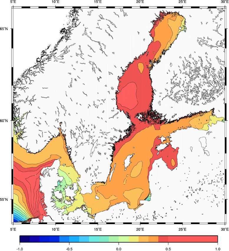
Die Küste, 92                                                    https://doi.org/10.18171/1.092103

gauges worked in Swinemünde since 1870 and in Arkona since 1872 (Birr 2005), stick
gauges were commonly used. Their readings were not always unambiguous. For example,
the pilot ladder for Travemünde quotes 3.41 m above mean sea level as maximum water
level on November 13, 1872, while the district administrator notes 3.26 m above mean sea
level (Anonymous 1872). Baensch (1875) reports 3.32 m above mean sea level for Novem-
ber 13, 1872, 2 p.m.
    Uncertainties of the same order result from the reduction of gauge data to mean sea
level, for example from the more general problem of defining mean sea level. Seibt (1881)
based his calculation of the mean water levels for coastal gauges on observation periods of
different lengths. More recent studies on the reference level were used by Mudersbach and
Jensen (2009). An updated study on the subject is given by Dangendorf et al. (2022).
Baensch (1875) relates a maximum error of 0.1 m to this kind of problem. An additional
error in using stick gauges resulted from their partly primitive attachment, so that they
became unusable after severe ice formation (Meyer 1871).
    Colding (1881) constructed a first set of contour maps of water level for the entire Baltic
Sea and the eastern North Sea from gauge measurements and other data at seven different
times during the period from November 12 to 13 (e.g. Figure 5b). In doing so, he interpo-
lated between available data. With regard to Colding's continuation of the lines of equal
water level into the open North Sea, it must be noted that the contemporary representation
of the tides followed a misconception by Airy (1845), although a more correct approach
had already been published by Whewell (1836) (after Cartwright 1999).
    Baensch (1875) and Colding (1881) have drawn the temporal development of the water
level at many places. While Baensch (1875) also gives the underlying data in tabular form,
Colding (1881) only notes the numerical values in his maps. Lentz (1879) graphically evalu-
ates the same water level records as Baensch (1875), probably independently of the latter.
Lentz (1879) presents graphically surge data for Cuxhaven and, in tabular form, water level
data for Copenhagen. In addition to these main papers, Pralle (1875) compares water levels
in Kiel and Husum. The Swedish Meteorological and Hydrological Institute, SMHI, has
related water level records in Öland Norra Udde to NN (cf. Figure 9 in Rosenhagen and
Bork 2009). There is also information on the water level at Grönskär, an island in the
Stockholm archipelago. The longest time series are those for Stockholm (since 1774) with
daily measurements for 1872 (Ekman 1988, Rosenhagen and Bork 2009) and for Kronstadt
(since 1804). In today's data sets for Kronstadt, the gauge records for 1872 are missing
(Klevanny 2008, personal communication). However, Bogdanov et al. (2000) give monthly
mean values for 1872. Numerical values are also given in the maps of Colding (1881). For
Cuxhaven, water level records exist since 1841 (Müller-Navarra et al. 2013). For November
1872, however, only high tide (HW) and low tide (NW) readings were taken, but not during
the night. These historical data were corrected to NN at BSH. The surge values given by
Lentz (1879) obviously make use of the same data. For Den Helder, the tides were related
to NAP (NN-NAP=+0.02 m) by Rijkswaterstaat.
    Based on this information, the maximum water levels on the German Baltic Sea coast
during the storm surge of 1872 have been repeatedly compiled and evaluated (Krüger 1910,
Jensen and Töppe 1986, Baerens 1998, Baerens et al. 2003, Mudersbach and Jensen 2009).
The values of the water level measurements vary considerably in some cases e.g. due to
registration time. Even when the highest water level was determined according to tide
marks and witness statements, the values differ.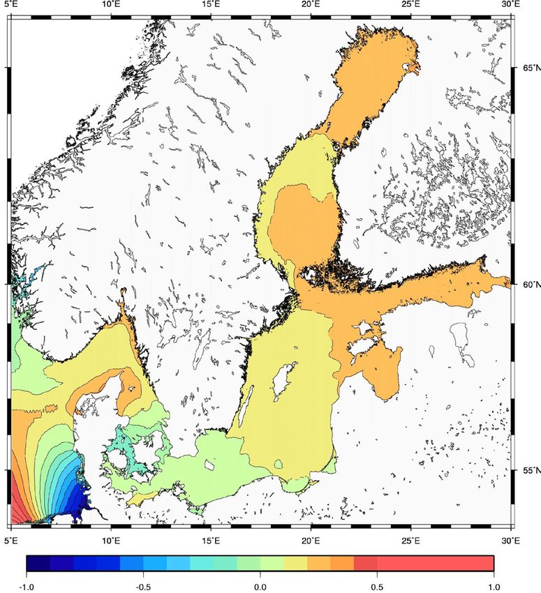
Die Küste, 92 https://doi.org/10.18171/1.092103
2.2 Previous work on air pressure and wind
The storm surge of 1872 coincided historically with the establishment of national meteo-
rological services. Their measurements are taken into account in the historical considerations.
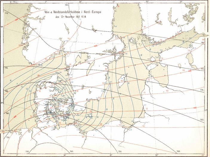
The most detailed contemporary elaboration of the storm surge is from Colding (1881).
He constructed a second set of maps for the entire Baltic Sea area. These show isopleths
of atmospheric pressure and wind direction as well as punctual information on wind direc-
tion and wind speed for the period from November 12 to 13, 1872 (e.g. Figure 1, left).
Another extensive early source is that of Baensch (1875), which describes the development
of the weather situation by means of maps of the morning air pressure fields for November
10 to 13, 1872 (e.g. Figure 1, right). The publication also contains extensive station-related
data on wind and air temperature, which are, however, limited to the Baltic Sea coasts of
the Prussian state. Later authors follow in their presentations either Colding (Hennig 1911
and 1919, Seifert 1952) or Baensch (Kruhl 1973, Thran and Kruhl 1972). Thran and Kruhl
(1972) in particular reconstructed weather maps in comparison to all four maps by Baensch.
The representations in Baensch (1875) and Colding (1881) for the morning of Novem-
ber 13, 1872 differ mainly in the presence of a low over the southern Baltic Sea. In Baensch
(1875) it is the remnant of a small-scale marginal depression that had been found north of
Berlin on November 10 and 11, 1872. It is important to note that the air pressure data used
by Baensch for the analysis of the isobars were not reduced to sea level, as necessary for
the exact comparability of the values. Although the Baltic Sea coastal region is predomi-
nantly rather flat, more or less small inaccuracies will exist.
Since van Bebber's (1891) publication on frequent tracks of low-pressure systems over
Europe, the weather situation that led to the flood of 1872 has been described with great
agreement in subsequent literature as a Vb situation (Hennig 1911 and 1919, Krüger 1910,
Kohlmetz 1967, Kruhl 1973). They describe a low-pressure system moving on the van
Bebber Vb track from the Adriatic Sea around the eastern side of the Alps to Central Europe.
Figure 1: Weather maps, November 13, 1872 in the morning, left: after Colding (1881), right: after
Baensch (1975).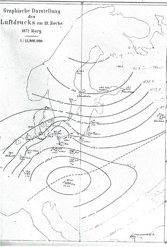
Die Küste, 92                                                        https://doi.org/10.18171/1.092103

3    Reconstruction
3.1 Procedures
The goal of this investigation, to clarify the causes of the extraordinary storm surge of 1872
on the basis of current meteorological and oceanographic knowledge with numerical mod-
els, required in particular a digital reconstruction of the meteorological fields. However, the
available 1872’s observed data are not sufficient for a reanalysis with a three-dimensional
numerical atmospheric model. Also the air pressure analysis available until 2009 from the
EU project EMULATE (Ansell et al. 2006) with mean daily values of the air pressure in a
5 degree grid obviously cannot explain the severe storm at November 13, 1872 in the area
of the western Baltic Sea. Therefore, the classical meteorological method was used: drawing
of weather maps, determining the geostrophic wind from the pressure fields and estimating
the wind at a height of 10 m. The more comprehensive “Twentieth Century Reanalysis”
(Compo et al. 2011), which was published later, recorded the meteorological situation be-
fore and during the Baltic Sea storm surge much better in terms of quality, but was still
inadequately in terms of quantity (Feuchter et al. 2013). This is due to the unchanged low
data base.

3.2 Analysis of air pressure fields
For the meteorological analyses, all available air pressure and temperature observation data,
independent of the evaluation status, of the period November 1 to 13, 1872 were requested
from the national meteorological services of Europe. The request resulted in collecting the
values from more than 230 observation stations (Figure 2), of which more than 175 had at
least two reports per day.

Figure 2: Stations with meteorological data available for the reconstruction.

In 1872, the metric system had not yet been introduced. Measurements of air pressure were
often in inch and feet, which had non-uniform regional length. The application of the data
therefore required after the digitization an extensive checking and standardisation of the
Die Küste, 92                                                    https://doi.org/10.18171/1.092103

differently evaluated data. The details of place and time were also not entirely comprehen-
sible. All air pressure data were put into a uniform status, reduced to sea level and converted
to hectopascal (hPa) and, regarding time, to UTC.
    The geographic distribution of the checked data collective was inconsistently dense.
Almost all air pressure values came from land or island stations (see Figure 2), with the
highest density over northern Germany. However, as with Colding (1881) and Baensch
(1875), there were hardly any ship’s observations from the North and Baltic Sea. This un-
even distribution of data with wide parts of areas without any information provides poor
prerequisites for a numerical interpolation. By tracking the weather situation over time with
meteorological experience, more accurate results can be achieved and readjustments in par-
ticular are made easier. In addition, the manual analysis offers the opportunity for a further
examination of the data and obvious wrong data could be eliminated.
    Since the oceanographic model system used later to calculate water levels requires wind
data as one driving force up to the northeast Atlantic, the daily mean values of air pressure
available from the EMULATE project (Ansell et al. 2006) were used as support. The num-
ber and distribution of the available data allowed three manual analyses per day for the
European land areas as well as for the North Sea and Baltic Sea for the period from No-
vember 1 to 11, 1872 and six each for November 12 and 13.
    The hand drawn isobars were then digitised with the help of the geo information system
ArcGIS (ESRI 2004) and interpolated to a geographical grid of 0.5 degrees grid width. For
control purposes, the generated grid point data were then evaluated again as isobaric fields.
    The results showed partly unrealistic structures, especially at the outer edges. By chang-
ing to natural neighbour (in space) interpolation, this kink could later be largely eliminated
(Kählke 2011, ESRI 2009).

3.3 Derivation of wind fields
For each grid point of the 0.5-degree grid, the geostrophic wind was calculated from the
pressure values of the four surrounding grid points. The method bases on the balance of
the Coriolis force and the pressure gradient force (Alexandersson et al. 1998). Above 100 m
height, this approximation determines the real wind to 90 % to 95 % (Möller 1973). Since
the pressure gradient force is inversely proportional to the distance between the isobars,
the geostrophic wind can be calculated solely from the air pressure distribution.
    However, this does not take into account the influence of friction on the rough surface
(land or sea), which causes a rotation of the wind and a reduction of the wind speed. For
the ageostrophic change in wind direction at sea, an angle of 30 degree was chosen after
test simulations regarding the water level. When the wind blows from land onto the sea,
the slowing effect of the rough land surface is noticeable near the coast. In addition, greater
roughness also causes an increase in the ageostrophic angle of the wind direction. As the
storm on November 13 came from the north-east, it blew mainly over water in the central
Baltic Sea, but also over southern Sweden and the Danish islands. Taking into account the
distance of the grid points to the coast could incorporate such effects. But they were neither
considered in the estimation of the wind speed at 10 m height nor later in the forcing in
the oceanographic model. An error estimate cannot be given.
    For the wind speed at a height of 10 m, empirical approaches exist whereby the reducing
influence of friction can be estimated. A comparison of the approaches of Duun-Christensen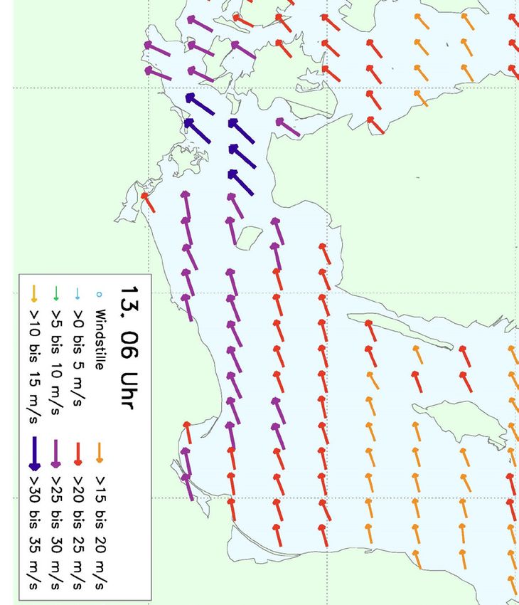
Die Küste, 92                                                    https://doi.org/10.18171/1.092103

(1975), Hasse (1974) and Luthard and Hasse (1981 and 1983) showed a great sensitivity to
thermal stratification, represented here by the difference between air and water tempera-
ture.
   Since the storm surge of 1872 was accompanied by a massive cold spell (seen in the air
temperature data), the bottom winds calculated according to the approach of Hasse (1974),
which takes into account the temperature difference of water and air, gave the best agree-
ment with the observed values and provided the decisive water level increase in the ocean-
ographic model. For the estimation of the temperature stratification, the air temperature
data of the collected archival data of the national meteorological services were used. For
the water temperature, climatological monthly mean surface temperature values for No-
vember (Janssen et al. 1999) were applied.

3.4     Derivation of water level
The simulation of the storm surge of 1872 was carried out with the operational model
system of the BSH (Kleine 2004, Dick et al. 2008), which takes into account the influence
of the Northeast Atlantic and the North Sea on the water level of the Baltic Sea. Numeri-
cally, the model system at that time was based on finite differences with grid spacing of
0.9 km in the western Baltic Sea and the German Bight, 5 km in the rest of the North Sea
and the Baltic Sea, and 10 km in the Northeast Atlantic. Vertically, generalised coordinates
were used with up to 25 layers in the western Baltic Sea and the German Bight, 30 in the
rest of the Baltic and North Sea and one in the Northeast Atlantic.
    The Northeast Atlantic was described by a two-dimensional barotropic model. In the
area of the North and Baltic Sea, a baroclinic three-dimensional model calculated the prog-
nostic variables of layer thickness, horizontal current, temperature, salinity, ice thickness
and ice compactness. Vertical current velocity and water level are then diagnostic variables.
All prognostic variables require initial and boundary conditions.
    The most important boundary condition here is the momentum input at the surface. In
the area of the North Sea and Baltic Sea it is determined from the reconstructed 10 m
winds. The parameterisation of the wind shear uses the linear approach for the wind shear
coefficient of Smith and Banke (1975) for wind speeds up to 30 m/s. For higher wind
speeds, the wind shear coefficient is kept constant. The above-mentioned change in inter-
polation method for the air pressure fields resulted in slightly higher maximum wind speeds
and thus higher peak water levels for the western Baltic Sea. We compensated for this in
the oceanographic model by reducing the wind speed threshold in the wind shear coeffi-
cient parametrisation from 30 m/s to 25 m/s.
    The approach of Smith and Banke (1975) for the wind shear coefficient applies to neu-
tral temperature stratification. The existing instability during the flood period is thus only
taken into account in the estimation of the 10 m wind from the geostrophic wind. Since
only the water level was to be simulated, the complex construction of air temperature fields
from the data was dispensed with. Instead, the heat flux from air to water was calculated
by setting the air temperature explicitly equal to the temperature of the water surface.
    To drive the northeast Atlantic barotropic model, only wind values, derived from
EMULATE data were used. Although very inaccurate, this simulates an inflow from the
northeast Atlantic into the North Sea, especially during the first 10 days of the investigated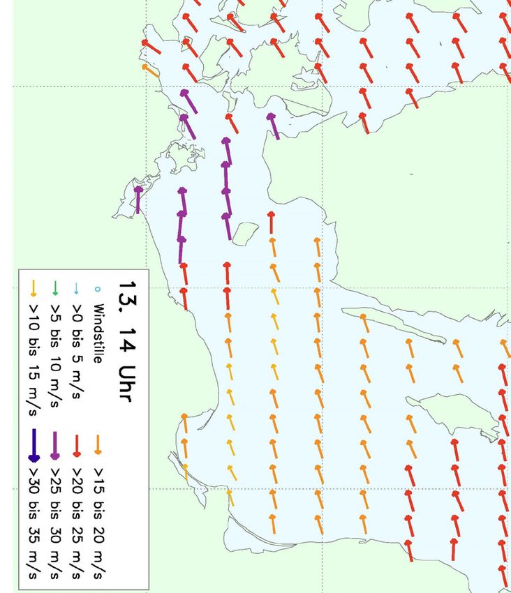
Die Küste, 92                                                      https://doi.org/10.18171/1.092103

period. The resulting boundary values for the North Sea were accordingly not included in
the iteration process to adjust pressure to water level.
    Tides are accounted for in the model equations via the potential of the tide-generating
forces as direct tides (Müller-Navarra 2002). Co-oscillation tides are prescribed at the open
north respectively west edge of the North Sea in the form of 14 partial tides. The corre-
sponding constituents were added for 1872. The model results usually are in UTC. How-
ever, this is only important regarding tides. That they were correctly adjusted to 1872’s data
is seen for example in results for Flensburg and Husum (Figure 3a and Figure 8). The
meteorological forcing is given in UTC.
    The initial state of temperature and salinity was described by climatological November
values (Janssen et al. 1999). Accordingly, only relative changes in salinity during the first 10
days of the simulation are accounted for. Such information could be understood as an
indication of water transport but were not evaluated. No attempt is made to interpret the
relative temperature fields either.
    More importantly, only climatological values can be used for river inputs. However, we
are not aware of any extreme inflows in the period under consideration (Krüger 1910). It
is further assumed that the Baltic Sea was ice-free at the beginning of the simulation on
November 1, 1872. During the simulation period, no ice formed in the model due to the
inaccurate estimate of the heat flux, despite the cold spell mentioned.
    A particular problem arises with regard to the water level. On the one hand, the water
level in the model is related to an equipotential surface of the gravity, while, the measured
data, on the other hand, is related to the mean sea level. This results in a necessary correc-
tion of modelled water level up to −0.422 m (St. Petersburg) for the Baltic Sea. In detail,
the mean model sea level shows different horizontal deviations from the “mean water
level”. Accordingly, the initial distribution for the water level, which determines initial layer
thickness, was constructed from annual mean values of the operational model for 2002 and
the daily mean value of November 1, 1872 at Landsort. There are no gauge values for
Landsort for 1872, but there are for Grönskär. According to Colding (1881), the water level
there was 0.0 m on November 1. This value is also assumed for Landsort. For details and
references compare Bork and Müller-Navarra (2009a, chapter 3.1.1).

4    Verification
4.1 Wind
The data of wind direction and wind speed at 10 m were calculated directly from the geo-
strophic wind independently of the known observed values. Their verification was thus
possible with the available observations of wind force and direction from the coastal sta-
tions of the Baltic Sea. For this purpose, a comparison was made between the values of the
coastal stations and the nearest sea point of the reconstructed wind grid data set. The wind
observation values of the coastal stations (three observation times per day) were taken from
the publication by Baensch (1875, Tables I to IV). The wind directions there were indicated
in different angular spacing. There are stations with 8 and with 16 direction classes. For
Flensburg, this less detailed data from table IV was also used for verification. The wind
speed is given in a 6-level scale. An assignment to wind speed classes could only be roughly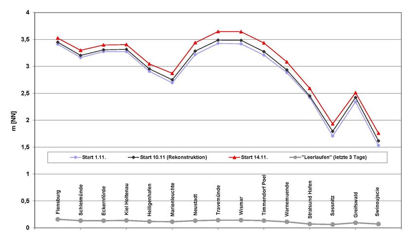
Die Küste, 92                                                      https://doi.org/10.18171/1.092103

estimated. The values given in Table 1 were used to convert the wind forces to speeds in
metres per second.
Table 1: Wind scale used by Baensch (1875) and its conversion to wind speed in m/s.
                    Wind scale (Baensch)     Converted wind speed classes
                             0                         0−2 m/s
                              1                         3−9 m/s
                              2                        10−14 m/s
                              3                        15−20 m/s
                              4                        21−28 m/s
                              5                         > 29 m/s

In any way, deviations are to be expected between wind observations at coastal stations
and values calculated for nearby sea points. In addition, there are the mentioned uncertain-
ties due to the standardisation of the collected air pressure values as well as finally the
freedom of interpretation in manual air pressure analysis. In addition, especially the con-
version method between geostrophic and 10-meter wind via the empirical approaches and
the estimation of the thermal stratification necessary for this involves multiple simplifica-
tions.
    A very effective check of the wind grid data was finally carried out indirectly by com-
paring the water level simulated by the oceanographic model system with the existing gauge
data. While the reconstructed wind fields for the period from November 1 to 11, 1872
showed satisfactory agreement with the gauge data at the first attempt, the water level from
November 12 onwards reacted sensitively and with large changes in the peak water level to
relatively small changes in the pressure field. Although the overall shape of the water level
curves matched during the first test run, the maximum heights did not. Eight modifications
of the pressure field resulted in only minor changes. At last, a significant improvement was
achieved by taking into account the thermal stratification when calculating the 10-m wind
from the geostrophic wind. The change in the course of the iterations is shown for
Flensburg in Rosenhagen and Bork (2009).
    There remains, however, another problem. Numerous dam breaches and water ingress
into the hinterland (e.g. Hemmelsdorfer See) on the Baltic Sea coast caused the water level
to fall despite a persistent storm (Quade 1872, Griesel 1921). Where this is registered by
gauges, the effect would enter the iteration and reproduce data on water level that modify
the local wind in an ambiguous way. Therefore, no such locations were taken into account.
    A comparison of the observed and the reconstructed winds for four Baltic Sea stations
is shown in Table 2. Despite the simplified calculation methods, there is very good overall
agreement both in terms of direction and speed of the wind during the time considered.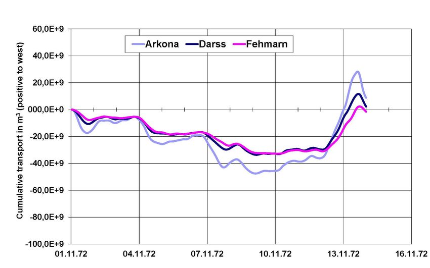
Die Küste, 92                                                                             https://doi.org/10.18171/1.092103

Table 2: Wind direction and force from observed data (left columns B) according to Baensch
(1875), and from the reconstruction at the nearest grid point at sea (right columns R) for Flensburg,
Lübeck, Putbus and Swinemünde between November 1 and 13, 1872.
                Nov.1872           Flensburg                 Lübeck                  Putbus                     Sw inem ünde
                day   hour   direction    force       direction   force       direction       force       direction      force
                              B     R    B     R       B     R    B   R       B      R    B       R        B      R     B      R
                1      6           SW             3    W    W     3       2   SW    W     3           3   WSW WSW       2        2
                1      14          WSW            2    W    WSW   2       3    -    SW    3           2   WSW WSW       2        2
                1      22          SSW            1    W    SSW   2       1   SW    SW    2           2   WSW    SW     2        1
                2      6           SSW            3   WSW   SW    3       2   S     SW    2           2   SSW SSW       2        2
                2      14          SSW            2    W    SW    3       1   S     SW    2           1   WSW SSW       2        3
                2      22           S             2    W     S    3       2   SE    SW    2           1   SW     SSW    2        3
                3      6           SSW            1    W    SSW   3       2   S     SW    2           1   SW     SSW    1        3
                3      14          WSW            1   WSW WSW     3       2   S     W     3           1   WSW WSW       3        2
                3      22          WSW            2   WSW   W     3       2   W     W     3           2   SSW WSW       2        2
                4      6           WSW            3    W    W     1       2   W     W     3           3    W     WSW    2        3
                4      14          W              2   NW    W     2       1   W     W     3           2   NW      W     2        2
                4      22          SW             1   NW    WSW   1       1   SW    W     2           1   WNW WSW       1        1
                5      6            S             2    W    SSW   2       2   S     SW    1           1   SW     WSW    1        1
                5      14           S             2   SW    SSW   2       3   SE     S    2           1   SW      S     2        3
                5      22          WNW            1   SSW   W     1       1   SE     S    2           1   SW     SSW    1        3
                6      6           SW             1   WSW WSW     1       1   W           2           0   NW     WSW    1        1
                6      12    SW          1
                6      14          W              1    W    WSW   1       2   SE    SW    2           1    W     SW     1        3
                6      22          SW             3   WSW WSW     3       2   S     SW    2           2   WSW    SW     1        2
                7      6           SW             3    W    WSW   3       3   SW    W     3           3   WSW WSW       3        3
                7      12    SW          4
                7      14          W              2    W    WSW   3       2   SW    W     3           3    W     WSW    4        3
                7      22          SW             2    W    WSW   3       1   SW    W     3           3    W      W     3        2
                8      6           SW             2    W    WSW   1       2   W     SW    2           2    W     WSW    1        3
                8      12    WSW         2
                8      14          W              2    W    WSW   2       1   SW    SW    2           1   WSW WSW       3        1
                8      22          W              1    W    WSW   2       1   SW    W     2           1   WSW WSW       2        2
                9      6           W              2    W    WSW   1       1   W     W     1           2    W      W     1        1
                9      12    SW          1
                9      14          W              2   WNW WSW     2       1   SW    W     2           2    W     WSW    1        1
                9      22          SW             1   WNW   SW    1       1   S           1           0    W     SW     1        1
                10     6           SW             1    W    WNW   1       1   S     SE    1           1   SE     SSW    1        2
                10     12    SW          0
                10     14          SE             0    W    SSE   1       1   SE     N    1           1    E     ENE    1        1
                10     22          SE             0    -    NNE   0       1   W     NW    1           1   NE     NNW    1        1
                11     6            E             1   ENE   ENE   1       1   NW     N    1           1    -      N     0        2
                11     12    NE          1
                11     14           N             1   ENE   NNE   2       1   N     NE    1           1   NE     NNE    1        1
                11     22          NE             1   ENE   NE    2       2   NE    NE    2           1   NE     ENE    1        2
                12     6           NE             2   ENE   ENE   3       2   N     NE    2           3   SE     ENE    4        2
                12     ß8          NE             2
                12     12    NE          4
                12     14          NE             3   ENE   NNE   4       3   NE    NE    3           3   ENE     NE    4        3
                12     22          NE             2   ENE   NNE   4       5   NE    NE    4           4   ENE    ENE    4        3
                13     0           NE             3
                13     6            N             4   ENE   NE    4       4   NE     E    5           5   ENE    ENE    5        4
                13     8            N             4
                13     12          NE             4
                13     14          NE             4   ENE   NE    4       3   E      E    3           4    E      E     4        3
                13     18          NE             3
                13     22           E             3   ESE   ENE   3       3   E      E    2           3    E     ESE    4        4
Die Küste, 92 https://doi.org/10.18171/1.092103
4.2 Water level
The water level observations cannot be used for the verification of the model simulations,
as some of the observations were used to modify the constructed air pressure field towards
a better modelling of the gauge measurements. That this was achieved satisfactorily is
shown by the time series in Figure 3a-c and the peak water levels (Figure 4). This is less
true for water levels in the remaining Baltic Sea. A comparison for Ölands Norra Udde is
given in Rosenhagen und Bork (2009).
In the North Sea, the data for Den Helder and Cuxhaven are not reproduced despite
error correction (for potential causes compare Janssen 2002). In contrast, the agreement
for Husum is very good (Figure 8). Finally, in Figure 5a, a spatiotemporal distribution of
the water level is given in comparison to one of the first set of maps by Colding (1881) in
Figure 5b, which presents contours of water level together with lines indicating wind direc-
tion.
In figures and tables historical data are with respect to mean local water level (MW) in
1872 and local time, while model data are corrected in height to account for differences of
model zero to NN (Mudersbach and Jensen 2009, Bork and Müller-Navarra 2009a, 3.1.2).
Furthermore, model values are always extracted at a grid point near the station where meas-
urements were taken, compare Bruss and Bork (2009, Figure 2).
Table 3 demonstrates the variation of data and includes corrections to model results for
some stations. In Figure 5a model water levels are corrected in similar way as initial values.
Table 3: Extreme water levels evaluated by different authors (Baensch 1875, Baerens 1998,
Mudersbach and Jensen 2009 Table 1) and corrections applied.
Baensch Baerens Mudersbach
Gauge Correction
1875 1998 2009
[m MW] [m MW] [m NN 2006] [m]
Flensburg 3.31 3.08 3.27 −0.164
Schleimünde 3.44 3.21 −0.169
Eckernförde 3.15 3.40 −0.167
Kiel Holtenau 3.17 2.97 3.30 −0.169
Neustadt 2.95 2.82 −0.195
Travemünde 3.32 3.30 3.15 −0.195
Wismar 2.84 2.97 −0.195
Warnemünde 2.45 2.70 −0.216
Stralsund Ha-
2.46 2.41 2.56 −0.245
fen
Greifswald 2.64 2.66 2.79 −0.246
Furthermore, the time of model data is corrected to local time, assuming one hour differ-
ence to UTC.Die Küste, 92 https://doi.org/10.18171/1.092103 Figure 3a: Water level at Flensburg. Observations (m MW, local time, red) from Baensch (1875), November 6 to 20, 1872 and corrected model data (m NN, blue), November 1 to 13, 1872. Figure 3b: Water level at Travemünde. Observations (m MW, local time, red) from Baensch (1875), November 6 to 20, 1872 and corrected model data (m NN, blue), November 1 to 13, 1872.
Die Küste, 92                                                    https://doi.org/10.18171/1.092103

Figure 3c: Water level at Stralsund. Observations (m MW, local time, red) from Baensch (1875),
November 6 to 20, 1872 and corrected model data (m NN, blue), November 1 to 13, 1872.

From Figure 3a-c it also is obvious that level readings not always coincide with time of
maximum water level. E.g. for Flensburg and Travemünde there are only three readings
during the time of the storms: November 12, midday, November 13, 4:30 p.m. and No-
vember 14, midday. For Stralsund and other places in the Bay of Mecklenburg there is
additional information around the time of peak value of the flood. The most detailed ob-
servations exist for Kiel Holtenau (Figure 8).

Figure 4: Peak water levels. Corrected model data (m NN, blue), observations (m MW, red) from
Baensch (1875) for different places along the German Baltic coast, November 13, 1872.
Die Küste, 92 https://doi.org/10.18171/1.092103
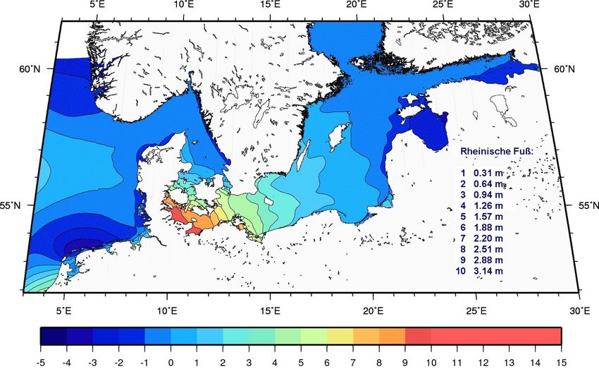
Figure 5a: Corrected water level on November 13, 1872, 2 p.m., converted to Rhenish feet for
comparison to Figure 5b.
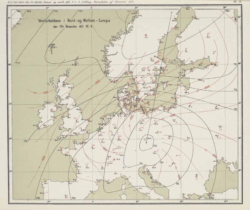
Figure 5b: Contours of water level in Rhenish feet (blue), atmospheric pressure (black) and lines
indicating wind direction (red) on November 13, 1872, 2 p.m. (Colding 1881).
5 Weather pattern before and during the storm surge
5.1 Historical descriptions
In addition to measured and observed values, there are various contemporary descriptions
of the weather before and during the storm surge.
The information on the course of the weather in November 1872 is incomplete, but in
part quite differentiated. According to Quade (1872), there was severe gale from NE ob-
served in Warnemünde as early as November 12. Hurricane-force wind from NE startedDie Küste, 92 https://doi.org/10.18171/1.092103
there at midnight and turned to SE on November 13 around 2 pm. In Stralsund and
Swinemünde (Swinoujscie), both storm and hurricane-force wind blew from NE (Baensch
1875). Krüger (1910) emphasises the change in wind direction of the extreme wind on
November 13 from ENE east of Rügen to NE west of Rügen. In the attempt to explain
the unusually high-water levels of 1872, later authors greatly simplify the course of the
weather. Kiecksee (1972) writes about southwestern winds over the entire Baltic Sea from
November 1 to 10, which intensified into a storm in the period from November 6 to 9.
From November 10 in the evening to November 11 in the morning, he constructs a phase
of calm over the entire Baltic Sea, followed by a wind from northeast, which increased to
a storm in the course of November 12. Afterwards, he follows the description of Baensch
(1875) for November 13, according to which gale-force winds first appeared around 2 a.m.
at Colbergmünde (Kolobrzg) and reached Kiel (Ellerbeck) at 7 a.m. on November 13.
Contemporary explanations of the meteorological event are partly pictorially descriptive
and are hardly sufficient to clarify the causes of the three-dimensional event. Baensch
(1875) describes in detail a battle of polar and equatorial air masses. Kohlmetz (1967) and
other authors explain the strong winds over the Baltic Sea from the Vb-weather situation.
Baensch (1875) additionally outlines a secondary low over the river Oder.
5.2 Results of the reconstruction
The reconstruction of the weather situation of the period considered results in a rough
division into three phases for the southern Baltic Sea, similar to the description in the his-
torical sources:
November 1 to 9: prevailing westerly and south-westerly winds,
November 10: weather change,
November 11 to 13: increasing easterly winds with storm up to hurricane-force from north-
east over the western Baltic Sea on November 13.
More details on the weather situation before and during the storm surge for the period
from November 1 to 13, 1872 are presented in Rosenhagen and Bork (2009).
Contrary to what was predominantly described, the reconstruction does not explain the
storm situation as the result of a typical Vb weather situation. Rather, on November 10, an
extensive low-pressure system with two centres moved from the North Sea towards Central
Europe. While the eastern centre shifted eastward, the western part migrated south-east-
ward towards Central Europe. There it remained until after November 13. Between No-
vember 10 and 12 the Central European low hardly intensified. Only with the inclusion of
an Adriatic low-pressure area in the night of November 13 a rapid deepening to pressure
values below 995 hPa occurred. Compare Figure 6b. Since November 11, the low over
Central Europe was confronted with increasing high air pressure over Northern Europe,
with the centre of the high slowly moving towards Central Scandinavia. In the second half
of the day on November 12, the Scandinavian high intensified to more than 1045 hPa.Die Küste, 92 https://doi.org/10.18171/1.092103 Figure 6a: Reconstructed air pressure fields on November 13, 6 a.m. (left) and 2 p.m. (right). This resulted in an extreme air pressure gradient over the entire southern Baltic Sea leading to wind speeds of gale-force and more. Compare Figure 6b. While a north-eastern storm raged in the western part, easterly wind directions prevailed over the central and eastern areas of the southern Baltic Sea. Figure 6b: Reconstructed wind distribution on November 13, 6 a.m. (left) and 2 p.m. (right), Wind- stille = calm). Further wind distributions around 6 h, 3 h before and at the time of the peak water level for Flensburg, Travemünde and Greifswald can be found in Bork and Müller-Navarra (2009b) in comparison with the wind fields causing extreme surges calculated in project MUSE-Baltic-Sea. 6 Numerical Experiments In the project MUSE-Baltic Sea, a total of 31,800 realizations of potentially extreme weather conditions were calculated using an ensemble prediction system (EPS) at 37 target dates (Schmitz 2009). Following a preliminary investigation (Bruss et al. 2009), 15 of these
Die Küste, 92                                                                 https://doi.org/10.18171/1.092103

were finally used to drive the model system of the BSH (Northeast Atlantic, North Sea and
Baltic Sea).
   In Bork and Müller-Navarra (2009b), the focus of the investigation was on a compari-
son of these extreme storm floods with that of 1872. Here the statements on the storm
flood of 1872 are detailed.
   In all figures, model values are always extracted at a grid point near the station where
measurements were taken, compare Bruss and Bork (2009, Figure 2).

6.1 Motivation
The popular scientific image of the storm surge of 1872 is shaped by early ideas and roughly
corresponds to the picture that Krüger (1910) draws of the typical course of a storm surge
in the western Baltic Sea.
     “Just as the high tide is preceded by a low tide, so too are the wind-generated tides in the western Baltic
Sea. It is stormy SW to W (WNW) wind that creates these low tides on the coasts of the western Baltic
Sea. They drive the water away from our coasts into the northern part of the Baltic Sea, filling it up and
often creating storm surges on the Russian coasts.
     These westerly winds, which cause low tide on our coasts, as soon as they prevail at the entrance to the
Baltic and North Sea − here best as westerly to north-westerly − cause a current moving from N to S
through the Sound and the Belts and thus an inflow of water from the Kattegat, further from the North
Sea and the Atlantic Ocean into the Baltic Sea, then − preferably south-westerly winds − a further filling
of the northern Baltic Sea.
     These strong W to SW winds filling the northern Baltic are caused by deep (pressure) minima taking
their migration north of us across Scandinavia or across the Baltic in a roughly west-easterly direction (the
stormy weather on the right-hand side of the depression track!).
     If, after a long period of strong westerly blowing winds, a strong N to NE wind suddenly develops, the
water masses are driven back from the northern Baltic Sea and thrown particularly against the southern
coasts of the western Baltic Sea, causing severe flooding here.
     A hydrological sign of these storm surges is a rise in the water level on the southern coasts of the western
Baltic Sea even with westerly winds, a sign that the northern Baltic Sea is already completely filled, so that
a reverse flow had to occur despite the adverse winds.
     If this sign is accompanied by a rapid rise in the barometer as a second (meteorological) sign with westerly
winds after it had previously shown a very low level, the residents of the western Baltic Sea can count on a
storm surge. The rise in the barometer indicates an air pressure maximum approaching from NE, which
in connection with a low minimum approaching from the Atlantic (very low barometer reading!) caused the
strong N to NE storms and thus the storm surges in the western Baltic Sea are.”
    The controversy in contemporary and more recent literature about the causes of the
very high-water levels during the storm flood of 1872 also reflects aspects of this idea.
    Since the hurricane-force wind on November 13, 1872 was devastating in its conse-
quences, but according to contemporary information not completely exceptional in its
strength, some authors suspect additional causes for the very high-water levels of 1872: in
an increased mean water level of the entire Baltic Sea (Baensch 1875, Kiecksee 1972,
Baerens 1998), in an increased return transport caused by wind (Grünberg 1873, Kiecksee
1972, Weiss and Biermann 2005). According to Grünberg (1873), this then leads to an
extreme increase in the water level in the western Baltic Sea due to winds that prevent
Die Küste, 92 https://doi.org/10.18171/1.092103
outflow into the North Sea. Other authors also discuss an unfavourable interaction with
the Kattegat (Pralle 1875, Eiben 1992). It was also occasionally postulated that the storm
on November 12, 1872 contributed to the high-water levels (Kiecksee 1972).
Colding (1881), on the other hand, emphasizes the sole effect of the storm for the flood
on November 13, 1872. Krüger (1910) blames the turning of the hurricane-force wind as
it progresses west for the particularly high water levels on the coast of Schleswig-Holstein.
Lentz (1879) points out the particular expansion of the wind field. Recent investigations
also suggest that the spatial extent of the strong wind band could have had a maximizing
effect (Irish et al. 2008).
In addition to an increased filling level of the Baltic Sea, compensating processes such
as seiches of the entire Baltic Sea are discussed as increasing causes for extreme storm
floods (Meinke 2003, Fennel and Seifert 2008). Contemporary literature on the storm flood
of 1872 also speaks of swinging back, supported by the effects of the wind (Grünberg 1873,
Baensch 1875). Sager and Miehlke (1956), on the other hand, find no evidence of large-
scale seiches in connection with extreme events.
6.2 Influence of the water level of the central and northern Baltic Sea
The calculations by Colding (1881) were later given little credit and in a German summary
(Anonymous 1882) the translator noted the additional influence of a “Vorfluth” (previous
filling of the Baltic Sea) in a footnote. The emphasis on the mean water level of the central
and northern Baltic Sea is probably related to the beginning understanding of the circula-
tion of the Baltic Sea (Meyer 1871). Today's ideas about the circulation of the Baltic Sea are
more differentiated.
An overview of the physical conditions in the Baltic Sea including tides, storm surges
and swell can be found in Feistel et al. (2008). The discussion presented here focuses on a
storm flood in the western Baltic Sea consisting of the Bay of Kiel and the Bay of
Mecklenburg. These parts of the Baltic Sea are flat and, together with the Kattegat, Belts
and Sound, are part of the multi-connected transition area between the North Sea and the
Baltic Sea. Of significant importance for the physical exchange processes are the Great
Belt, the Fehmarn Belt, the Sound and the shallow sills (Darss and Drogden Sill) as bounda-
ry to the Arkona Sea and the central Baltic Sea (Jacobsen 1980).
Particularly important for the dynamics of storm floods in the western Baltic Sea is the
short-term barotropic exchange across the sills and through the Belts and the Sound. In
large-scale storm conditions, it reaches the order of magnitude of 105 m³/s or 0.1 Sverdrup
within a few hours (Müller-Navarra 1983, Lass and Matthäus 2008).
The inflow from the North Sea and the Atlantic is also emphasized in the quotation
above (Krüger 1910). Weidemann (1950) outlines the position of the high- and low-pres-
sure areas for optimal inflow and outflow conditions. In fact, the reconstruction shows air
pressure distributions that favour an inflow, especially on November 4, 1872 (Rosenhagen
and Bork 2009). However, the exchange rates between the western and central Baltic Sea
change direction several times in the reconstruction at the level of Arkona. The maximum
transport (15-minute average) from the western Baltic Sea is reached on November 4, 1872
with 4.4·105 m³/s or 0.44 Sverdrup. A similarly high outflow was also modelled for No-
vember 7, 1872. These values already show that a preconditioning “Vorflut” of the BalticDie Küste, 92 https://doi.org/10.18171/1.092103
Sea through wind induced water transport and its later effect on the peak water levels dur-
ing extreme storm floods is less important than the local wind accumulation on the flat
coasts together with swell.
For the argumentation in relation to the storm surge of 1872, the period over which an
inflow situation can last must be considered. Literature and reconstruction assume SW to
WNW winds up to November 10, 1872 in the Bays of Kiel and Mecklenburg. However,
wind speeds vary greatly during this phase (compare Table 2).
More clearly than transport rates, a cumulative transport [m3] describes the net flow
from and into the western Baltic Sea. For the reconstruction, Figure 7 shows cumulative
volume transports from the beginning of the simulation on November 1, 1872 for Fehmarn
Sound and Fehmarn Belt, across the Darss Sill and into the central Baltic Sea (Arkona).
The border to the central Baltic Sea was drawn from the east side of Rügen to Ystad in
Sweden (compare Bruss and Bork (2009) Figure 15 and Baltic Operational Oceanographic
System, BOOS, http://www.boos.org/transports/, section 29).
Figure 7: Cumulative transports (positive to the west) across sections at the level of Arkona (light
blue), the Darss Sill (dark blue) and of Fehmarn (Belt and Sound, red) between November 1 and
13, 1872. Vertical lines mark the beginning of each day.
The cumulative volume transport from the western to the central Baltic Sea reached its
maximum on the morning of November 9, 1872 with −47.5·109 m3. A significant decrease
in the net outflow into the central Baltic Sea begins with the storm on November 12, 1872.
At the beginning of the hurricane-force wind, the transport from the western Baltic Sea is
then compensated and during November 13, 1872 a net inflow from the central Baltic Sea
to the western Baltic Sea begins. It is at its maximum on the afternoon of November 13,
1872 with +28.2·109 m3. At the end of the reconstruction period it has already fallen to a
third of this value.
The cumulative transport across the Darss Sill ran parallel to that at Fehmarn for a long
time. Compared with Arkona, a significant decrease begins at about the same time, full
compensation, however, is achieved a little later. In contrast, the maximum cumulativeDie Küste, 92 https://doi.org/10.18171/1.092103
transport over the Darss Sill into the western Baltic Sea is reached at the same time, but is
significantly lower at +11.6·109 m3. Into the Bay of Kiel, a very short and minor cumulative
transport, at most +2.3·109 m3, occurs through the Fehmarn Belt and Fehmarn Sound.
In summary, the reconstruction shows that the cumulative transport into the central
Baltic Sea was determined by the air pressure distribution on November 4, 1872. and No-
vember 7, 1872. In the remaining time until the weather change on November 10 it kept
relatively constant. I. e. during such periods no substantial transport of water to or from
the western Baltic Sea took place. A positive cumulative transport from the central Baltic
Sea is only achieved with the hurricane-force wind on November 13, 1872. An increase in
the water level in the western Baltic Sea and especially in the Bay of Kiel “even with westerly
winds” (Krüger 1910, Grünberg 1873) cannot be explained by water transport from the
northern Baltic Sea.
Pralle (1875) and Eiben (1992) also found a rise in the water level before November 12,
1872, but suspect only an unfavourable interaction with the Kattegat as the cause. As evi-
dence of this, they cite the development of the water level in Husum and Kiel over time,
in which, from November 8, 1872, a steady decrease in the mean water level in Husum
corresponds to a steady increase in Kiel. Figure 8 shows the particularly well-documented
development of the water level in Husum and Kiel in comparison with the reconstruction.
According to the data, only the modelled high tides are given for Husum.
Figure 8: Observed high-tides at Husum (Pralle 1875) and water level at Kiel (Baensch 1875) for
November 1 to 15, 1872 compared to corresponding reconstructed values for November 1 to 13,
1872: observations (m MW, local time, red), reconstruction (corrected, m NN, blue).Vertical lines
mark the beginning of each day.
6.2.1 Experiment 1
Despite the above results of the reconstruction, the idea persists that long-lasting favoura-
ble winds could have led to the central and northern Baltic Sea being filled in at the begin-
ning of November 1872 (Vorflut) and later contributed to an increase in the water level in
the western Baltic Sea.
Therefore, in a numerical experiment, the wind distribution of November 4, 1872 was
assumed to be stationary for the period from November 4 to 14, 1872. The associated airDie Küste, 92 https://doi.org/10.18171/1.092103
pressure field (see Rosenhagen and Bork 2009) led to the maximum inflow rate into the
central Baltic Sea during the reconstruction period, but only lasted there for a short time.
After the water level in Landsort no longer increased, and even decreased slightly, the
meteorological forcing was switched off in the entire model area on November 14, 1872
and calculations continued until the water level curve in Landsort flattened out significantly
on December 2, 1872.
Figure 9: Left: Corrected water level in m NN in the Baltic Sea after 10 days of steady meteoro-
logical forcing. Right: Corrected water level of the reconstruction in m NN in the Baltic Sea at
November 10, 1872.
Figure 9 shows the water level across the Baltic Sea at the end of the steady meteorological
forcing compared to that during the reconstruction at the start of the weather change. The
latter is significantly lower, in the central Baltic by about 0.2 m. In the Gulf of Bothnia, the
difference is most pronounced. There, the water levels in the experiment on the Swedish
coast reach values of over 0.5 m. These are clearly caused by the local, stationary wind on
the north side of the low-pressure area and are independent of the water transport from
the western Baltic Sea.
The reconstruction (Figure 9 right) also shows slightly increased water level (between
0.2 and 0.3 m) in the Gulf of Finland and Riga. The determination of its cause is difficult,
since at the time of the second increased transport rate into the central Baltic Sea (on No-
vember 7, 1872) there was a depression over northern Scandinavia which also favoured an
influx into these regions.
6.2.2 Experiment 2 and 3
As a contribution to the discussion about the influence of the degree of filling of the entire
Baltic Sea on the water levels after the reversal of the weather situation on November 10,
1872, two further numerical experiments are presented. The reconstruction from Novem-
ber 10 to 13, 1872 was used as the meteorological forcing. Only the initial conditions forDie Küste, 92 https://doi.org/10.18171/1.092103
the water level were varied. This was realized by shifting the chronological assignment of
the meteorological data to the beginning of the reconstruction (November 1, 1872, EXP 2)
and the end of the filling experiment (November 14, 1872, EXP 3).
Figure 10a shows the development of the water level at Flensburg over time for the
reconstruction and the two experiments. Figure 10b shows the corresponding distribution
of the peak water levels. Experiment 2 starts with the initial state of the reconstruction on
November 1, 1872. The resulting peak levels hardly differ from the reconstruction itself
throughout. The greatest differences to the reconstruction are achieved in the third experi-
ment, which started with an artificially generated high filling of the Baltic Sea (start on
November 14, 1872), e.g. 0.16 m in Timmendorf on Poel and 0.08 m in Flensburg.
Figure 10a: Water level at Flensburg, for different initial conditions (blue EXP 2, red EXP 3) ap-
plying the meteorological forcing of November 10 to 13; compared to the reconstruction (black).
Vertical lines mark the beginning of each day.
Figure 10b: Peak water levels for different initial conditions (blue EXP 2, red EXP 3) applying the
meteorological forcing of November 10 to 13; compared to the reconstruction (black). Below, the
peak water levels during the last 3 days of the “emptying phase” from experiment 1 are included.Die Küste, 92 https://doi.org/10.18171/1.092103
In summary, it can be said that steady winds in the central Baltic Sea, which favour the
inflow into the Baltic Sea, simulate higher water levels than in the reconstruction, but such
winds are not observed for a long time. Rather, BOOS (http://www.boos.org/transports/)
shows transport rates that have been documented for many years (daily average, inflow
into the central Baltic Sea positive) for November, for example 2021, also briefly changing
transport directions.
Finally, a clarification of terms is useful. “Vorflut” in the older literature describes a
wind-related event with a spatially inhomogeneous rise in the water level, which completely
filled the northern Baltic Sea in 1872 (Grünberg 1873; Baensch 1875). “Vorfüllung”, on
the other hand, is understood as an increase in the water level throughout the Baltic Sea.
The degree of “Vorfüllung” is well captured by the water level at Landsort. In MUSE-
Baltic Sea, periods during which the mean water level in Landsort exceeds 0.15 m above
sea level over 20 days were defined as periods with increased fill levels (Mudersbach and
Jensen 2009). It should be noted that the water level in Landsort shows a clear annual
variation with a range of 0.216 m, a maximum in December, which on the average was
0.084 m and a relative minimum of 0.048 m in November when considering data from the
years 1899 to 1992 (Hupfer et al. 2003, local values corrected for eustatic changes). In 1872,
during the reconstruction, starting on November 1, the value of 0.15 m was exceeded sev-
eral times, but only for a short time in each case. Data are not available for Landsort. In
the data from Norra Udde and Nedre Stockholm (see Rosenhagen and Bork 2009), the
reference value of 0.15 m was exceeded only once up to November 10, 1872.
A climate-related rise in the sea level of the Baltic Sea is not discussed in connection
with the storm flood of 1872. Krüger (1910) assigns the major storm floods up to 1904 to
wet or dry periods (according to Brückner 1890) and finds that the majority of these storm
floods, and especially that of 1872, occurred during a dry period.
6.3 Impact of the storm on November 12 on the peak water level 1872
Colding (1881) explains the water level in the Baltic Sea during the storm on November
13, 1872 as a direct result of the wind alone. To do this, he draws lines of equal water level
based on collected data and compares them with values from wind data according to a
relationship he had derived earlier. His formula corresponds to today's ideas, but neglects
the Ekman transport (Ekman 1905). However, his maps also contain lines of wind direc-
tion. Noticing that the water level increases perpendicular to the wind direction and not
parallel, he corrects his calculations accordingly and finds his theory confirmed.
The assumption is occasionally made in the literature (Kiecksee 1972) that the surge
caused by the storm on November 12, 1872 contributed significantly to the increased water
level during the hurricane-force storm on November 13, 1872. Enderle (1989) studied the
time that elapsed between the onset of a storm and the peak water level in Flensburg. For
storms from the north and from the east over the central Baltic Sea it is about 7 hours
including the time that elapses between the wind picking up and the first water level change
at a specific location. For storms over the western Baltic Sea, such delay disappears. For
locations in the Bay of Mecklenburg, Miehlke (1990) calculated the time it takes a long
wave on the optimal path (greatest depth) after a storm over the central Baltic Sea to con-
tribute to the local surge. The times are between three and eight hours, depending on the
starting point. These estimates confirm a statement by Baensch (1875), according to whichDie Küste, 92 https://doi.org/10.18171/1.092103
the water level at the end of the storm on November 12 has reached a steady state in the
western Baltic Sea.
6.3.1 Experiment 4
In experiment 4, the question is investigated whether a surge caused by the storm of No-
vember 12, 1872 increases the surge caused by the hurricane-force wind. Contradicting,
there is the assumption that an existing stationary surge and the associated circulation make
it more difficult to increase the corresponding water level further (Jeffreys 1923 and Heaps
1965).
Based on the water level at the end of the filling experiment (EXP 1, cf. Figure 9 left),
simulations were carried out with the meteorological conditions of November 10 to 13
(EXP 4c) and of November 12 to 13 (EXP 4b). Finally, the conditions of November 13,
1872 alone were used (EXP 4a).
The difference in water level resulting from EXP 4c, which only neglected the phase
before the weather change and the experiment driven by the complete meteorological forc-
ing of the reconstruction, shows only slight differences in the peak water levels for all lo-
cations.
At Flensburg, the surge exclusively caused by the hurricane-force wind on November
13 exceeds the surge caused by a combination of the preceding storm and the one on
November 13 and thus confirms theoretical considerations. The result for Flensburg is
representative for the Bay of Kiel. In other places, the corresponding peak values are well
below those caused by both storms.
Figure 11: Water level at Flensburg according to EXP 4a (hurricane-force wind only, turquoise,
13.11.), EXP 4b (both storms only, petunia, 12.11.), and to EXP 4c (both storms including the
meteorological forcing after change in wind direction, red, 10.11.). Vertical lines mark the begin-
ning of each day.
Experiment 4 confirmed the thesis that the storm the day before rather had a hindering
influence on the surge caused by the hurricane-force wind on November 13, only concern-
ing results in the Bay of Kiel. The reasons for the different dynamic behaviour in the Bay
of Mecklenburg (Travemünde to Warnemünde) were not examined in detail. A possibleYou can also read