Modelling water-harvesting systems in the arid south of Tunisia using SWAT
←
→
Page content transcription
If your browser does not render page correctly, please read the page content below
Hydrol. Earth Syst. Sci., 13, 2003–2021, 2009
www.hydrol-earth-syst-sci.net/13/2003/2009/                                                        Hydrology and
© Author(s) 2009. This work is distributed under                                                    Earth System
the Creative Commons Attribution 3.0 License.                                                           Sciences

Modelling water-harvesting systems in the arid south of Tunisia
using SWAT
M. Ouessar1 , A. Bruggeman2 , F. Abdelli1 , R. H. Mohtar3 , D. Gabriels4 , and W. M. Cornelis4
1 Institut
        des Régions Arides (IRA), Route de Jorf, 4119 Medenine, Tunisia
2 International
              Center for Agricultural Research in the Dry Areas (ICARDA), P.O. Box 5466, Aleppo, Syria
3 Department of Agricultural and Biological Engineering, Purdue University, West Lafayette, IN 47907, USA
4 Department of Soil Management – International Centre for Eremology, Ghent University, Coupure links 653,

9000 Ghent, Belgium
Received: 10 March 2008 – Published in Hydrol. Earth Syst. Sci. Discuss.: 9 July 2008
Revised: 30 April 2009 – Accepted: 29 September 2009 – Published: 29 October 2009

Abstract. In many arid countries, runoff water-harvesting        served daily rainfall and runoff data. Recommendations for
systems support the livelihood of the rural population. Little   future research include the installation of additional rainfall
is known, however, about the effect of these systems on the      and runoff gauges with continuous data logging and the col-
water balance components of arid watersheds. The objective       lection of more field data to represent the soils and land use.
of this study was to adapt and evaluate the GIS-based water-     In addition, crop growth and yield monitoring is needed for
shed model SWAT (Soil Water Assessment Tool) for simulat-        a proper evaluation of crop production, to allow an economic
ing the main hydrologic processes in arid environments. The      assessment of the different water uses in the watershed.
model was applied to the 270-km2 watershed of wadi Kou-
tine in southeast Tunisia, which receives about 200 mm an-
nual rain. The main adjustment for adapting the model to this
                                                                 1   Introduction
dry Mediterranean environment was the inclusion of water-
harvesting systems, which capture and use surface runoff for
                                                                 Water management is the most critical issue in dry areas
crop production in upstream subbasins, and a modification
                                                                 as it impacts the livelihood of people and the productivity
of the crop growth processes. The adjusted version of the
                                                                 of the land and the society in general. For thousands of
model was named SWAT-WH. Model evaluation was per-
                                                                 years, inhabitants of the dry areas have constructed water-
formed based on 38 runoff events recorded at the Koutine
                                                                 harvesting systems that helped them cope with water scarcity
station between 1973 and 1985. The model predicted that
                                                                 (El Amami, 1984; Boers, 1994; Oweis et al., 2004). These
the average annual watershed rainfall of the 12-year evalu-
                                                                 systems were built to capture surface runoff from sparsely
ation period (209 mm) was split into ET (72%), groundwa-
                                                                 covered, rocky mountain slopes or to divert occasional wadi
ter recharge (22%) and outflow (6%). The evaluation co-
                                                                 flow to fields for crop production. Despite the long and suc-
efficients for calibration and validation were, respectively,
                                                                 cessful history of these systems, little is known about their
R 2 (coefficient of determination) 0.77 and 0.44; E (Nash-
                                                                 effect on the hydrological processes in these dry areas.
Sutcliffe coefficient) 0.73 and 0.43; and MAE (Mean Ab-
                                                                    Southeast Tunisia provides a typical example of the in-
solute Error) 2.6 mm and 3.0 mm, indicating that the model
                                                                 tensive management of scarce water resources in southern
could reproduce the observed events reasonably well. How-
                                                                 Mediterranean drylands. In this region, communities tra-
ever, the runoff record was dominated by two extreme events,
                                                                 ditionally constructed earthen dikes with small spillways
which had a strong effect on the evaluation criteria. Dis-
                                                                 across the wadis to harvest the surface runoff from the sur-
crepancies remained mainly due to uncertainties in the ob-
                                                                 rounding degraded mountain slopes in the upstream areas.
                                                                 The soil that built up behind the dike formed a terrace that is
                                                                 used for cropping. These ancient water-harvesting systems
                    Correspondence to: M. Ouessar                are referred to as jessour. Water harvesting gradually also
                    (med.ouessar@ira.agrinet.tn )                expanded to the foothills of the mountains, especially during

Published by Copernicus Publications on behalf of the European Geosciences Union.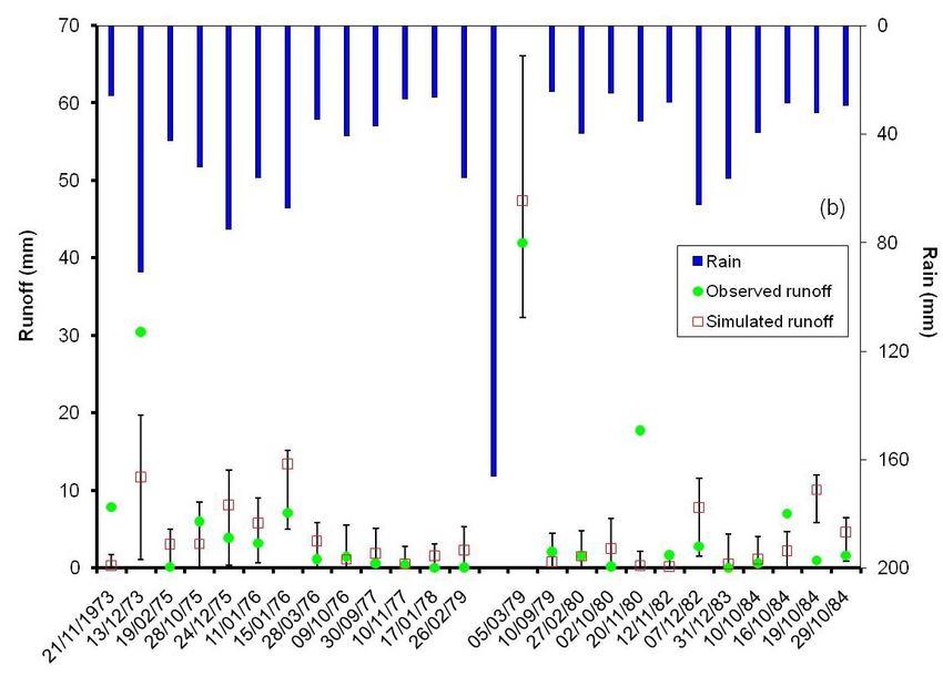
2004                                                                  M. Ouessar et al.: Modelling water-harvesting systems

the last three decades. Here earthen dikes were made in the      sights into the distribution and uses of water over space and
gently sloping plains to harvest the runoff from the adjacent    time and under different management practices. Although
mountain slopes. These so-called tabias are often built in se-   there are many watershed models (Singh and Woolhiser,
quence, with spillways to distribute the water evenly among      2002; Borah and Bera, 2004), few of them can be easily ap-
them. Thus, these water-harvesting systems intercept surface     plied to simulate the highly spatially and temporally variable
runoff from adjacent land units for crop production (mainly      processes in arid watersheds. Furthermore, there is no model
drought-tolerant olive trees) on broad terraces in upstream      that can simulate the functioning of the water-harvesting sys-
catchments, while this water would have flowed downstream        tems in these arid watersheds, where runoff water from one
through the wadi otherwise.                                      land unit is captured for crop production by a downstream
   Over time researchers have tried to obtain a better under-    land unit inside the same subbasin, with excess runoff water
standing of the water resources and their uses in this water     flowing again further downstream.
scarce environment. Between 1973 and 1985 a runoff sta-             The Soil and Water Assessment Tool (SWAT), developed
tion was established at the outlet of the 272-km2 Koutine        by Arnold et al. (1998), was selected for the simulation
watershed. During this relatively wet period, the 209-mm         of hydrological processes in arid watersheds with water-
average annual rainfall over the watershed produced an aver-     harvesting practices, because (1) it simulates all water flows,
age runoff of 12 mm/yr (6% of the rain), which flooded the       water balance components and crop yields of different land
downstream rangelands in the coastal plain (sebkhas) (Fersi,     units at various temporal scales (daily and long-term); (2) it
1985). The runoff water improved the productivity of these       allows easy representation and use of spatially variable data,
lands, which are the traditional grazing grounds of camels,      processes and results through a GIS interface; and (3) it has
sheep and goats. However, in dry years (e.g., 1981/1982), no     a wide development and users’ community with open access
runoff reached the downstream areas.                             to the model documentation and source code. Although a
   Transmission losses of the runoff that flows through the      cell-based routing procedure, as opposed to SWAT’s semi-
wide wadi bed are serving as a source of recharge for the        distributed approach at the subbasin level, would have been
region’s aquifers. The magnitude of groundwater recharge         more suitable for modelling flows in arid environments, the
was assessed by Derouiche (1997). She computed the               above strengths were considered to outweigh this weakness.
recharge of the 725-km2 Zeuss-Koutine aquifer, which un-            Applications of SWAT in watersheds in humid regions
derlays most of the wadi Koutine watershed, using biannual       have been abundantly published in the literature (e.g., Srini-
and annual groundwater level observations in 28 piezome-         vasan et al., 1993; Srinivasan and Arnold, 1994; Cho et al.,
ters and boreholes and the finite difference groundwater flow    1995; Bingner et al., 1997; Arnold et al., 1999; Santhi et al.,
model MULTIC (Djebbi, 1992). Lateral inflow from the up-         2001; Kaur et al., 2003). However, applications of SWAT
stream aquifer in the south (Grès de Trias) (30 l/s) and di-    in dry environments are still relatively limited. In Tunisia,
rect recharge in the Matmata mountains (4 l/s) were assumed      Bouraoui et al. (2005) applied SWAT to an 8000-km2 basin
constant and were estimated by calibration, whereas recharge     of the Medjerda river located in a semi-arid to sub-humid
from the remainder of the soils was assumed negligible. For      bioclimate (297–1056 mm annual rainfall) in the northwest
the period 1974/75 to 1984/85, average annual groundwa-          of the country to study the potential hydrological and wa-
ter recharge from wadis and the Matmata mountains (upper         ter quality (nitrate) impacts of land management scenarios.
boundary of the model) was computed to be equal to 301 l/s.      They found that the model was able to represent the hydro-
This would be equal to 13.1 mm over the area of the aquifer      logical cycle even though some discrepancies were observed,
and 6% of the average annual rainfall for this period in the     due to a lack of sufficient rainfall data but also due to the
wadi Koutine watershed.                                          fact that reservoirs (dams) were not simulated. In Morocco,
   The above two studies indicated that approximately 88%        Chaponniere (2005) applied SWAT for the representation of
of the rain that falls on the watershed ends up as evapo-        the hydrological functioning of a semi-arid mountain water-
transpiration. However, the evapotranspiration process is not    shed. She studied two theoretical scenarios on the poten-
equally beneficial over the watershed. Whereas the lush olive    tial effects of changing the partitioning between rainfall and
tree cover on the water-harvesting units indicates a produc-     snow on the outflow. She pointed out that one of the reasons
tive use of the water, evaporation losses from the degraded,     for the poor functioning of the model was the fact that the
sparsely covered soils of the rangelands are high.               local water-spreading systems (seguias), which have an im-
   Local authorities have requested researchers to provide       portant effect on the water routes inside the watershed, were
them with better information to help them understand the         not represented in the model. She recommended the inte-
effectiveness of different support measures on the distribu-     gration of these systems for any further analysis of the water
tion of the water in these dryland watersheds for competing      balance. Conan et al. (2003) applied SWAT (version 99.2) to
up- and downstream uses and users: (i) mainly rainfall and       demonstrate the impact of groundwater withdrawals on the
surface runoff for olive production and rangelands and (ii)      hydrological behavior of the Upper Guadiana catchment lo-
groundwater for domestic uses, agriculture, industries and       cated in a semi arid area (400–500 mm rainfall) of central
tourism. Watershed models are key tools for providing in-        Spain. They found that although the model is well adapted to

Hydrol. Earth Syst. Sci., 13, 2003–2021, 2009                                   www.hydrol-earth-syst-sci.net/13/2003/2009/
M. Ouessar et al.: Modelling water-harvesting systems                                                                        2005

describing the changes from wetlands to drylands due to hu-           In addition to the presence of shallow aquifers (less than
man interventions, it did not properly represent all the details   50 m deep) as groundwater beneath the main wadis of the wa-
of the discharge history. They recommended including ad-           tershed (Hallouf, Nagab, Koutine), the study watershed cov-
ditional rainfall data and reservoir operating information to      ers partially the sandstone Triassic aquifer (Grès de Trias) (in
enable better representation of the hydrological functioning       the upstream part) and the Zeuss Koutine aquifer (in the mid-
of the watershed. To evaluate the effect of different land uses    dle and downstream parts). The first one provides the fresh-
and management practices on surface and soil water flow in a       est groundwater of the region (salinity less than 1 g/l), which
small arid catchment in northern Syria, Bruggeman and Van          is mainly used for irrigation and drinking water salinity ad-
der Meijden (2005) adapted SWAT by introducing a number            justment (mixing with more saline water), while the second
of adjustments to the model including growth and dormancy          one is the main source of water supply for the province of
of olives and winter crops, the effect of grazing on leaf area     Médenine (Ouessar and Yahyaoui, 2006).
index (LAI), the change of Curve Number (CN) during the               The land use of the study area is dominated by sparsely
growing season, and the use of the “irrigation from reach”         covered, degraded steppes. Cropped sites, mainly for grow-
option to represent the runoff harvesting practices widely         ing olives, are found on terraces behind water-harvesting
used in typical dry environments of North Africa and West          structures. Two types of water-harvesting techniques are
Asia.                                                              practiced by the local farmers: jessour and tabias (Ouessar
   The overall objective of this paper is to adapt and eval-       et al., 2006).
uate SWAT for simulating the main hydrologic processes in             As described in the introduction, jessour are mainly found
arid Mediterranean environments. The specific objectives are       in the mountainous areas of the watershed. This ancient
to (i) develop a methodology to represent water-harvesting         water-harvesting technique is widely spread in the region of
systems in SWAT; (ii) adjust the crop model parameters and         the Matmata mountains. Jessour are constructed in the inter-
processes to represent Mediterranean arid cropping systems;        mountain and hill water courses to intercept runoff and sed-
(iii) evaluate the new SWAT-WH version in a 270-km2 dry-           iments. Jessour is the plural of a jessr which is a hydraulic
land watershed in southeast Tunisia using 38 storm events;         unit made of three main components: a dike (locally called
and iv) assess the magnitude of the water balance compo-           also tabia) in the form of a small earth embankment with a
nents (infiltration, percolation, transmission losses, outflow,    spillway made of stones, a terrace which represents the crop-
and evapotranspiration) for different land uses.                   ping area, and an impluvium which is the runoff catchment
                                                                   area (El Amami, 1984) (Fig. 2). The dikes are between 2
                                                                   to 5 m high and have lengths between 15 to 50 m across the
2     Materials and methods                                        wadi (Ben Mechlia and Ouessar, 2004).
2.1    Study area                                                     Tabias are essentially situated in the piedmont areas in
                                                                   the middle of the watershed on gentle slopes. The tabia is
The study watershed, wadi Koutine, is located in the Jef-          formed by a principal embankment of 50 to 150-m situated
fara region in southeast Tunisia. It lies in the upper arid        along the contour with lateral bunds of about 30 m long at the
bioclimate region (Floret and Pontanier, 1982). The rainfall       ends. The tabia gains its water directly from its impluvium
regime is of Mediterranean type with the rainy season ex-          or by the diversion of wadi runoff. Water is captured until
tending from September to April. The average annual rain-          it reaches a height of 20 to 30 cm, after which it is diverted
fall ranges from 160 mm in Médenine (1900–2004) in the            (over flow), either by a spillway or at the upper ends of the
Jeffara plain to 235 mm at Béni Khédache (1969–2003) in          lateral bunds (Alaya et al., 1993) (Fig. 2).
the Matmata mountains. The average annual temperature is              During rainfall events, the runoff that is generated at the
20◦ C, the coldest month is December (mean minimum daily           level of the impluviums runs onto the terraces of the jessour
temperature 7◦ C) and the warmest month is July (mean max-         and tabias. Part of the runoff water will form temporary
imum daily temperature 37◦ C).                                     ponds up to the level of the spillway. It will infiltrate into
   A runoff gauging station was established by the hydrologi-      the soil slowly after the runoff event. The jessour cover the
cal service of the Ministry of Agriculture (DGRE) in 1971 at       tributaries (talwegs), and receive runoff from the mountains
the crossing point between wadi Koutine and the main road          (mountain rangeland). The tabias receive the runoff from
linking Médenine and Gabès (Fersi, 1985). The watershed          their impluviums and/or the spillover from the upstream jes-
upstream from the runoff station covers an area of 272 km2         sour if they are installed on the same tributary. The outflow
and stretches from an elevation of 690 m above sea level           from the jessour and tabias flows into the wadi.
(a.s.l.) in the Matmata mountains to 100 m a.s.l. at Koutine
village and then extends downstream into the saline depres-        2.2   SWAT model
sion of Sebkha Oum Zessar before ending in the Mediter-
ranean (Gulf of Gabès) (Fig. 1).                                  SWAT is a physically-based continuous time model that op-
                                                                   erates on a daily time step to estimate the effects of land and
                                                                   water management and pollutant releases in stream systems

www.hydrol-earth-syst-sci.net/13/2003/2009/                                      Hydrol. Earth Syst. Sci., 13, 2003–2021, 2009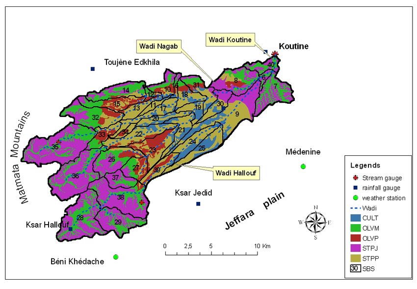
2006                                                                           M. Ouessar et al.: Modelling water-harvesting systems

Fig. 1. Study watershed location and monitoring network (OLVM: Olives of the mountains (jessour); OLVP: Olives of plains (tabias); STPJ:
Rangelands of the mountains; STPP: Rangelands of the plains; CULT: Cereals; SBS: Subbasin boundaries).
                      Figure 1. Study watershed location and monitoring network (OLVM: Olives of the mountains
                      (jessour); OLVP: Olives of plains (tabias); STPJ: Rangelands of the mountains; STPP:
in large complex watersheds with varying soils, land use and               level as required by the latter method, the SCS CN method
                      Rangelands of the plains; CULT: Cereals; SBS: Subbasin boundaries).
management conditions     over long periods of time (Neitsch               was selected for runoff computation. It calculates the runoff
et al., 2002). Spatial variability of soil, land use and man-              for a given rainfall depth and CN. It is an empirical formula
agement practices are accounted for by discretization of the               based on several years of rainfall and runoff data obtained
watershed into subbasins based on the topography and stream                from a variety of combinations of soil, land use, topography
network. Each subbasin consists of multiple Hydrologic Re-                 and climate across the US. The CN is related to the land use
sponse Units (HRUs) representing unique combinations of                    and the soil hydrologic group. The method is widely used,
soil and land cover properties.                                            not only in the US, but also in other countries (Ponce and
   The climatic variables consist of precipitation, maximum                Hawkins, 1996).
and minimum air temperature, solar radiation, wind speed,                     SWAT defines percolation as the water that drains through
and relative humidity. SWAT includes also the WXGEN                        the root zone into the aquifer. Downward flow occurs when
weather generator model (Sharpley and Williams, 1990) to                   the field capacity of a soil layer is exceeded. The downward
generate climatic data or to fill in gaps in measured records.             flow rate is governed by the saturated hydraulic conductiv-
For this study, the weather generator was only used to fill in             ity (Ks ) of the soil layer. Lateral subsurface flow in the soil
missing temperature data. The daily temperatures are gener-                profile is calculated simultaneously with percolation. A kine-
ated by WXGEN from user-defined monthly means and stan-                    matic storage routing method, which is based on slope, slope
dard deviations, using a weakly stationary process (Neitsch                length, and saturated hydraulic conductivity is used to predict
et al., 2002).                                                             lateral flow in each soil layer. Lateral flow occurs when the
   There are three options for estimating reference evapotran-             storage in any layer exceeds field capacity and is a function
spiration (PET): Hargreaves (Hargreaves and Samani, 1985),                 of lateral flow travel time (days) and the difference between
Priestley-Taylor (Priestley and Taylor, 1972), and Penman-                 soil water content and field capacity (Neitsch et al., 2002).
Monteith (Monteith, 1977; Allen, 1986). Considering the                       The lateral flow and surface runoff of all HRUs are
availability of data for the study area (minimum and maxi-                 summed for each subbasin and then routed through the
mum daily temperature), the PET was calculated by the Har-                 stream network. Transmission losses are computed as a func-
greaves method. Potential soil water evaporation is estimated              tion of the hydraulic conductivity of the channel bed (Kchan ),
as a function of PET and the plant’s LAI and plant water tran-             channel width and length, and flow duration, following the
spiration is simulated as a linear function of PET and LAI.                procedure of Lane (1983). SWAT routes the stream flow
   SWAT provides two methods for estimating surface runoff                 through the channel network using the variable storage rout-
volume: the SCS curve number procedure (SCS, 1972) and                     ing method or the Muskingum river routing method. Both
the Green and Ampt (1911) infiltration method. Because of                  methods are variations of the kinematic wave model as de-
the lack of long-term rainfall intensity data at the watershed             tailed by Chow et al. (1988).

Hydrol. Earth Syst. Sci., 13, 2003–2021, 2009                                            www.hydrol-earth-syst-sci.net/13/2003/2009/
M. Ouessar et al.: Modelling water-harvesting systems 2007
2.3 Model modifications
The main feature of jessour and tabias is that they receive
runoff water generated by different HRUs (degraded, rocky
rangelands) within the same subbasin. In SWAT, runoff is
not routed between HRUs within the subbasin, but the runoff
from all HRUs is added directly to the outlet of the subbasin.
The SWAT code was modified to simulate the collection of
runoff water behind the water-harvesting structures (jessour
and tabias) by bringing the surface runoff and lateral flow
generated in the subbasin back to the water-harvesting HRUs
in the subbasin (Fig. 3).
SWAT’s irrigation-from-reach option was used to allow
the entry of input data for controlling the amount of wa-
ter harvested by the different HRUs. Because the water-
harvesting units may not be located in such a way that they
capture all runoff that was generated within the subbasin, the
parameter FLOWFR allows the user to specify the fraction
of the runoff water that is harvested by the jessour and tabia
HRUs. The maximum height of the water impoundment on
each water-harvesting HRU is controlled by the height of the
dikes and spillway and the slight surface slope of the land
surface. This impoundment height is represented by the pa-
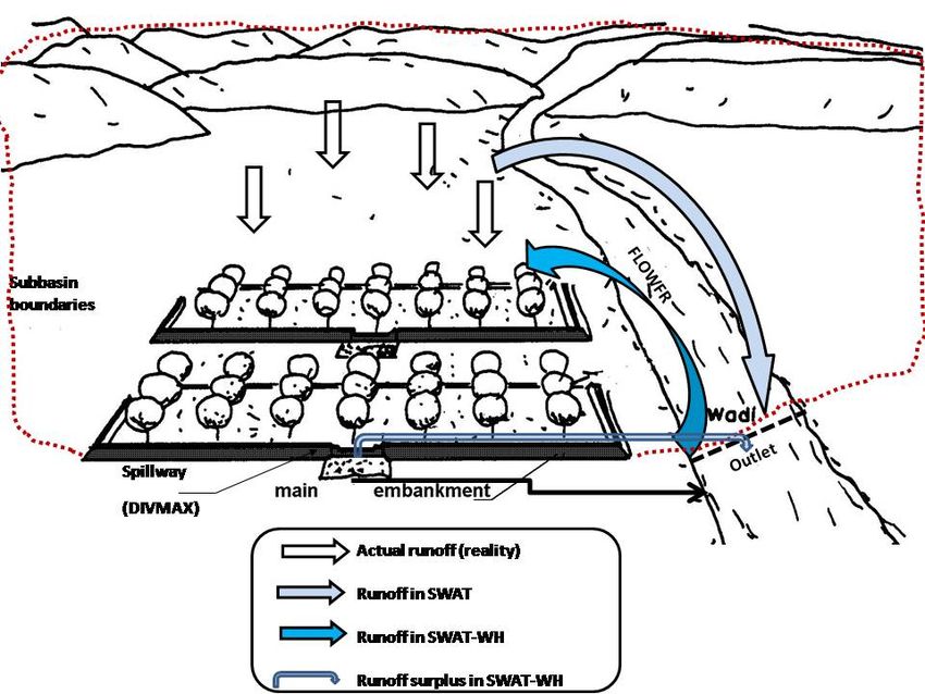
rameter DIVMAX, as illustrated in Fig. 4.
In subbasins with both water-harvesting systems, the jes-
sour are generally located upstream from the tabias. There-
fore, the runoff water is distributed to the jessour HRUs first
and secondly to the tabia units. Finally, any excess will flow
downstream and could be subjected to transmission losses in
the main reach (wadi).
Fig. 2. Uppper: scheme of the Jessr components (a spillway, b side The water-harvesting process for the jessour HRUs in a
view) (adapted from El Amami, 1984). Lower: scheme of a tabia subbasin is expressed by the following equations:
with natural impluvium (adapted from Alaya et al., 1993). In the
photo: tabias are seen in the front (piedmont area) and jessour are FLOWFR(i) × Qsub
found in the talwegs of the mountains in the back. DW = (2)
i=n
P
10 × AREA(i)
i=1
The crop growth and biomass production module uses a
DWH(i) = MIN(DW, DIVMAX(i)) (3)
simplified form of the EPIC crop model (Williams et al.,
1984). The model uses Monteith’s approach to estimate i=n
X
the potential biomass accumulation (Monteith, 1977), cou- QRE = QSUB − (DWH(i) × 10 × AREA(i)) (4)
pled with water, temperature and nutrient stress adjustments. i=1
SWAT simulates also erosion and water quality processes but
these are not considered in this application. where DW is an intermediate parameter for the height of the
Considering the above processes, the water balance of the harvested water on the water-harvesting HRU (mm), QSUB
soils and streams of the watershed can be expressed as fol- is the total runoff (surface runoff and lateral flow) generated
lows: in the subbasin (m3 /d), i is the index for the jessour HRUs
in the subbasin, n is the total number of jessour HRUs in the
1SW = P − QSURF + ET + WSEEP + QGW (1) subbasin, AREA(i) is the surface area of each jessour HRU
(ha), DWH(i) is the final height of the harvested water on
where 1SW is the change in soil water content, P is the pre-
the jessour HRU (mm) and QRE is the remaining runoff that
cipitation, QSURF is the surface runoff out of the watershed,
will flow downstream (m3 /d). The expression MIN(v1,v2)
ET is the evapotranspiration, WSEEP is the percolation from
indicates that the minimum of the two values will be selected.
the soil profile and QGW represent the transmission losses
It should be noted that within a subbasin the FLOWFR for all
from the streams. All parameters are expressed in (mm) over
jessour HRUs will be constant. The same equations are also
the watershed area.
used for the tabia HRUs. As explained above, in the case
www.hydrol-earth-syst-sci.net/13/2003/2009/ Hydrol. Earth Syst. Sci., 13, 2003–2021, 20092008 M. Ouessar et al.: Modelling water-harvesting systems
2.4.1 Topography and watershed configuration
A 30-m DEM was generated from available topographic
maps of the area (scales of 1:50 000; 1:100 000 and
1:200 000), from a SPOT stereo pair and from the stream
network digitized from a multi-spectral (XS) SPOT image,
using the TOPOGRIDTOOL routine. The main channel net-
work was created by the ArcView SWAT interface from the
DEM, using a threshold upstream drainage area, which de-
fines the head of a main channel, of 100 ha. Some of the
generated stream channels were removed to match the actual
occurrence of the streams as observed on the SPOT image.
Especially in the upstream areas the channels are completely
Fig. 3. SWAT water routing as applied in the study site (WH-HRU: covered by cascades of jessour. A few subbasins were sub-
water harvesting HRU, DIVMAX: maximum diversion (spillway divided, through the manual addition of outlets, to ensure the
height), FLOWFR:
Figure 3. SWAT flow
water routing fraction).
as applied in the study site (WH-HRU: water harvesting HRU, connection between runoff generating areas and the different
DIVMAX: maximum diversion (spillway height), FLOWFR: Flow fraction). cropped areas that harvest this runoff. In this way 35 sub-
basins were obtained.
of both jessour and tabias HRUs within the same subbasin, The main transmission losses are expected to take place at
the equations are applied to the jessour first and then to the the level of the main reaches (wadis). A value of 70 mm/h,
tabias with QSUB set equal to QRE . corresponding to the average effective hydraulic conductivity
If the total water harvested by the HRU exceeds the field of a channel with sand and gravel and low silt content (Lane,
capacity of the soil profile, it will become percolation. This 1983), was used. This value is also close to the average mea-
is different from the SWAT irrigation operation, which limits sured value (91 mm/h) found by Osterkamp et al. (1995) in
the water application to what can be stored in the soil profile. the United Arab Emirates for similar wadi bed properties as
The lateral flow of the jessour and tabias was assumed zero in the study watershed. The recharge from the wadis in the
(nearly level terraces). It is assumed that all harvested wa- upstream subbasins that are completely covered with jessour,
ter infiltrates in the soil, so no open water evaporation losses as well as from the tributaries in the subbasins, was assumed
are accounted for. This assumption seems reasonable, con- negligible (Kchan =0 mm/h).
sidering that generally only a few days ponding occur, during
humid conditions with relatively low temperature and cloudy 2.4.2 Climate
skies.
The second modification was the adjustment of the crop Daily precipitation data are needed when using the SCS
model parameters and processes to represent Mediterranean curve number method to model surface runoff. The daily
arid cropping systems. The initialization of the heat unit ac- rainfall data, recorded and published by the hydrological ser-
cumulation was changed to allow the perennials and annual vice of the Water Resources Directorate in the Ministry of
crops to grow during the Mediterranean hydrologic year from Agriculture (DGRE, 1968–1985), were collected from the
fall to summer. The dormancy period was removed because 7 stations (Koutine, Allamet, Toujène Edkhila, Ksar Hallouf,
the crops in the watershed do not become dormant. Fur- Ksar Jedid, Béni Khédache and Médenine) in and around the
thermore, as olives are permanently green, the shedding of watershed (Fig. 1). SWAT allocates the nearest rain gauge to
leaves for trees, present in the model, was removed. SWAT each subbasin. Due to some missing records, the rain gauge
allows the user to specify a change in CN for selected tillage allocation is different for the first 3 years of the 12-year eval-
practices, but this option did not function in SWAT2000; this uation period. Values of maximum and minimum tempera-
was corrected. The modified SWAT model is referred to as ture were obtained from the weather stations of Médenine,
SWAT-WH. Béni Khédache and El Fjè (IRA). The monthly average daily
minimum and maximum temperatures and standard devia-
2.4 Model parameterization tions of these stations were computed for use by the weather
generator to fill in missing data.
The new SWAT-WH was applied to the entire 272-km2 large
study watershed upstream from Koutine. We used a 12-year
2.4.3 Soils
runoff record (1973/1974 till 1984/1985) available for the
runoff station of Koutine (Fersi, 1985) for model testing and Soil classes were obtained from the soil map (at 1:200 000
evaluation. The values of the base parameter set (reference scale) of the Jeffara region produced by Taamallah (2003),
scenario) are discussed in this section, the selection of pa- based on a visual interpretation of a Spot multi-spectral
rameters for calibration is explained in Sect. 2.5. (XS) image of 1998 and field investigations. Texture of
Hydrol. Earth Syst. Sci., 13, 2003–2021, 2009 www.hydrol-earth-syst-sci.net/13/2003/2009/M. Ouessar et al.: Modelling water-harvesting systems 2009
Fig. 4. Schematic representation of the runoff routing in SWAT and SWAT-WH. DIVMAX: spillway height, FLOWFR: flow fraction.
Figure 4. Schematic representation of the runoff routing in SWAT and SWAT-WH.
DIVMAX: spillway height, FLOWFR: Flow fraction.
31 representative profiles was determined using the sieve- A summary of the soil characteristics is given in Table 1.
pipette method (Gee and Bauder, 1986) and organic matter It can be noted that the soils in the watershed are generally
by the method of Walkley and Black (1934). very shallow (10–40 cm), and have consequently limited wa-
The soil map was modified to take into account the soils ter holding capacity except the fluvisols (PEAH), which are
built up behind the water-harvesting units as deposited sedi- found in the northern, midstream part of the watershed, and
ments. The boundaries of the soil units were adjusted based the artificial soils created by the water-harvesting systems
on a supervised and unsupervised classification of the Spot (JESR and STAB).
XS image of 1991 and additional field investigations using
a handheld Global Positioning System (GPS). Three classes 2.4.4 Land use and CN
were added: the deep “artificial” soils formed as small ter-
races behind the water-harvesting structures by the deposi- A land use map of the study area based on a semi-supervised
tion of sediment (JESR: soils behind jessour, STAB: soils classification of the Spot XS image of 1991 (Zerrim, 2004)
behind tabias) and the calcareous outcroppings on the moun- was adjusted by adding the different soil and water manage-
tains, as part of the Matmata cuesta, in the upstream parts of ment practices (jessour and tabias), with the help of a visual
the watershed where the soil is almost nonexistent (AFFL). interpretation of the Spot XS image of 1998 and aerial pho-
For the soils on the terraces (JESR and STAB) of the tos (missions of 1975, 1990), in addition to field checks and
water-harvesting structures, measured available water capac- GPS surveys.
ity (AWC), bulk density (BD) and saturated hydraulic con- The main land uses in the watershed are rangelands, fruit
ductivity (Ksoil ) (Maati, 2001) were used. AWC was deter- trees and cereals. Fruit trees, mainly olives, (Olea Eu-
mined from the difference in soil-water content at −33 kPa ropaea), are found on the jessour and tabias only. Cereals
and −1500 kPa using pressure chambers (Soil moisture (barley, Hordeum vulgare, and wheat, Triticum durum) are
Equipment, Santa Barbara CA, USA). The BD was measured grown episodically during wet years. The natural vegetation
using 100-cm3 cores and Ksoil was obtained from infiltra- (ranges) was divided into two classes: mountain and plain,
tion experiments using a double ring with an inner diameter because of their different phenology and grazing practices.
of 28 cm and an outer diameter of 53 cm. As is frequently The soil hydrologic group and CN values were selected
done in watershed modelling where the soil properties are based on the SCS tables (SCS, 1986). Because of their
not fully available (e.g., Heuvelmans et al., 2004; Bouraoui shallowness, most soils were identified as group D soils,
et al., 2005), the missing water characteristics of the remain- defined as soils with very low infiltration rates, including
ing soils were derived by means of the calculator of Sax- shallow soils over nearly impervious material (SCS, 1986).
ton (2005). The rangelands were considered arid rangelands made of
www.hydrol-earth-syst-sci.net/13/2003/2009/ Hydrol. Earth Syst. Sci., 13, 2003–2021, 20092010 M. Ouessar et al.: Modelling water-harvesting systems
Table 1. Summary of the soil properties.
Soil* Depth Clay Silt Sand BD AWC K OC
cm % % % mg/m3 % (vol) mm/h %
AFFL 0–10 13 12 75 1.5 12 18 0.24
CRCG 0–20 10 9 81 1.6 10 29 0.28
MBEH 0–20 13 11 75 1.5 12 18 0.24
PEEH 0–20 11 11 78 1.6 12 24 0.29
ISOH 0–10 7 4 89 1.7 9 53 0.22
10–40 9 7 84 1.6 10 37 0.18
STAB 0–7.5 19 17 64 1.5 15 120 0.70
7.5–100 15 10 75 1.6 12 120 0.36
PEAH 0–70 10 15 75 1.6 12 28 0.12
70–140 3 19 78 1.8 12 84 0.15
140–200 16 17 67 1.5 13 11 0.19
JESR 0–7.5 15 21 64 1.4 18 60 1.02
7.5–52.5 17 19 64 1.5 18 60 0.51
52.5–200 14 14 72 1.7 14 17 0.28
AWC: available water capacity; BD: bulk density; K: Hydraulic conductivity; OC: organic carbon.
AFFL: Outcropping; CRCG: calcimagnésiques sur rendzine calcalire (Rendzinas); ISOH: isohumiques bruns calcaires tronqués (Calcic
Xerosols); JESR: soil on the terraces of jessour; MBEH: minéraux bruts d’érosion hydrique (Regosols); PEAH: Peu évolués d’apport
hydrique (Fluvisols); PEEH: peu évolués d’érosion hydrique (Regosols); STAB: Soil on the terraces of tabias.
∗ – in French: French classification (CPCS, 1967) (Taamallah, 2003);
– between parentheses in English: FAO classification (FAO, 1989).
herbaceous-mixture of grass and low growing brush (SCS, The characteristics of the US southwest rangelands were
1986), while the cereals were considered small grains in used with minor adjustments (biomass production, grazing
straight rows and bare soils during fallow. The olives are pattern, base and optimal growth temperature) based on re-
grown on flat terraces, with a CN of 30. search work undertaken in the arid regions of Tunisia (Floret
To allow a change in CN when the crops and rangelands and Pontanier, 1982; Neffati, 1994; Ouled Belgacem, 2006).
have developed a protective ground cover, a tillage operation The rangelands are generally grazed throughout the year by
with zero depth and zero mixing was used. For the range- various animals like sheep, goat and camel.
lands and cereals, the CN was set for three periods as a func- After the first significant rains, which fall between Octo-
tion of the growing cycles and management operations, and ber and November, the farmers plant barley and occasionally
included planting, grazing, harvesting (Table 2). wheat and legumes. Following harvest in May, the stubble of
cereals is completely grazed by the animals and only negligi-
2.4.5 Crop growth and management parameters ble amounts of residues are left. The cereal crop parameters
suggested by Bruggeman and Van der Meijden (2005) for
The crop parameters (potential heat units, base and optimal the Khanasser Valley (Syria) were adopted because of simi-
temperatures, length of the growing season, leaf area de- lar climatic dryland conditions.
velopment parameters) for the relevant crops in the SWAT As described previously, the water-harvesting systems are
database were checked and adjusted to obtain the general controlled by two parameters. The value of DIVMAX was
growth and water use patterns as observed in the study area. set to 0.25 m for the jessour and 0.15 m for the tabias, based
Although, for this study, the testing of the crop input and on field knowledge about average ponded water levels on the
output data focused on the effects of the soil water balance terraces of these water-harvesting systems (Chahbani, 1990;
rather than on the actual crop yields, some adjustments were Alaya et al., 1993; Ben Mechlia and Ouessar, 2004). Con-
made as described below. sidering that not all runoff water is captured by the water-
Olive trees are the dominant fruit trees cropped in the area. harvesting systems, the FLOWFR of jessour and tabias were
It was assumed that the olive trees have matured but kept set to 0.90 and 0.95, respectively. The jessour and tabias
growing normally by pruning the tree after harvest in Decem- have similar characteristics throughout the watershed, so
ber. The values of the radiation use efficiency and the harvest these values were assumed constant for all jessour and tabia
indices were adjusted to obtain biomass and yield produc- HRUs.
tion figures close to the average values found in the literature
(Labras, 1996; Fleskens et al., 2005) and field knowledge.
Hydrol. Earth Syst. Sci., 13, 2003–2021, 2009 www.hydrol-earth-syst-sci.net/13/2003/2009/M. Ouessar et al.: Modelling water-harvesting systems 2011
Table 2. Soil hydrological groups and base and final runoff curve number values, with the final values that were adjusted in the calibration
to the right of the oblique.
Landuse1 Soil2 Area (%)3 HYDGRP4 Curve Number
Mountain rangelands4 Oct–Nov Dec–Jun Jul–Sep
STPJ AFFL 4.4 D 97 97 97
STPJ CRCG 0.8 D 93/95 89/91 97
STPJ1 MBEH 26.3 D 93/95 89/91 97
STPJ ISOH 3.9 D 93/86 89/84 97/95
STPJ PEAH 0.1 A 80/63 71/55 84/77
Plain rangelands5 Oct–Nov Dec–Jun Jul–Sep
STPP CRCG 9.5 D 93/92 89 97
STPP MBEH 0.2 D 93/92 89 97
STPP PEEH 3.9 D 93/92 89 97
STPP ISOH 6.9 D 93/86 89/84 97/94
STPP PEAH 5.5 A 80/61 71/55 84/77
Cereals Nov–Dec Jan–Apr May–Oct
CULT CRCG 3.6 D 91 89/88 94
CULT PEEH 0.1 D 91 89/88 94
CULT ISOH 3.4 D 91 89/84 94/91
CULT PEAH 0.8 A 72/63 67/60 77
Olives Jan–Dec
OLVM JESR 22 A 30
OLVP STAB 8.6 B 30
1 CULT: Cereals; OLVM: Olives of the mountains (jessour); OLVP: Olives of plains (tabias); STPJ: Rangelands of the mountains; STPP:
Rangelands of the plains.
2 AFFL: Outcropping; CRCG: calcimagnésiques sur rendzine calcalire (Rendzinas); ISOH: isohumiques bruns calcaires tronqués (Calcic
Xerosols); JESR: soil on the terraces of jessour; MBEH: minéraux bruts d’érosion hydrique (Regosols); PEAH: Peu évolués d’apport
hydrique (Fluvisols); PEEH: peu évolués d’érosion hydrique (Regosols); STAB: Soil on the terraces of tabias.
3 As percentage of the watershed total area.
4 Hydrologic group as defined by SCS (1986); A: deep, well-drained, sandy soils with high infiltration rates; B: moderately deep to deep,
moderately fine to moderately coarse textured soils with moderate infiltration rates; D: shallow soils with very low infiltration rates.
5 For rangelands in the study area (O. Belgacem, personal communication, 2004):
– March–June: 25–50% cover,
– October–November: 10–25% cover,
– July–September:2012 M. Ouessar et al.: Modelling water-harvesting systems
interaction is captured. The relative sensitivity index (RSI) found between the total event runoff and the totals computed
(Lenhart et al., 2002) was computed as follows: from the daily data, which indicates that the accuracy of the
data may not have been very high. After 1979, rainfall in
(y1 − y0 )/y0
RSI = (5) Koutine, Allamat, Béni Khédache was recorded by a rainfall
(x1 − x0 )/x0 recorder. For this period, Fersi (1985) provided hyetographs
where x0 is the initial value of the parameter (baseline pa- for 6 events but with the rainfall averaged for the three sta-
rameters) and y0 is the corresponding output, x1 is the tested tions. A few inconsistencies were noticed between the rain-
value of the parameter and y1 is the corresponding out- fall event totals on the isohyets maps of Fersi and the totals
put. The sign of the index shows if the model reacts co- for the reported runoff period obtained from the daily rain-
directionally to the input parameter change, i.e. if an increase fall data reported by DGRE (1968–1985). Apparently, the
of the parameter generates an increase of the output and vice daily rainfall (08:00 a.m. to 08:00 a.m.) was not always con-
versa. A value of RSI near zero indicates that the output is sistently recorded on the correct day. After cross checking
not sensitive to the parameter under study, whereas a value between the above data sources and INM (1979–1985), daily
of RSI significantly different from zero shows high degree rainfall amounts of one or two stations were moved one day
of sensitivity Lenhart et al. (2002) classified the RSI sensi- backwards or forwards for a few events, based on the occur-
tivity values as follows: less than 0.05: small to negligible; rence and spatial distribution of the rain at the 6 rain gauges
0.05–0.2: medium; 0.2–1.0: high; more than 1: very high. in and around the watershed and the nearby Medenine station
The tested values of the parameters were their expected (Fig. 1).
upper and lower limits. Based on field knowledge, the DIV- A summary of the rainfall and runoff observations of the
MAX was changed up and down by 20% while the FLOWFR 38 observed runoff events used for the model evaluation is
was varied by 5%. The soils in the watershed are domi- presented in Table 3. Out of the 38 events, 31 had less than
nated by sandy loam textures, which have an expected AWC 5 mm runoff, with all peak flows below 60 m3 /s, while only
range of 6 to 12% (e.g., Allen et al., 1998). However, be- 3 events had more than 15 mm runoff. The two largest runoff
cause the total storage capacity of the soils is also affected events were recorded on 12–13 December 1973 (30 mm) and
by their depth, which involves another uncertainty, this pa- on 4–5 March 1979 (42 mm). This last event had a peak flow
rameter was varied with a 50% range. The changes for the of 1475 m3 /s. The magnitude of the peak flow was linearly
Ksoil were similar. For the Kchan , we used the range given by related to the total runoff. The duration of the events ranged
Lane (1983) and Osterkamp et al. (1995) (30 to 180 mm/h) between 6 and 54 h; there was no relation between the dura-
for typical dry channels. The range for the CN was 5% up tion of the events and the total runoff.
and 10% down. Because the CN values in the watershed are The highly variable behaviour of the watershed is evi-
relatively high (see Table 2), a 10% increase would exceed denced by the watershed runoff coefficients (runoff divided
theoretically feasible CN values, with CN=100 representing by precipitation). Although the intensity of the rain plays a
a completely impermeable land cover. role in the runoff behaviour of the watershed, as indicated
The model was run by changing one parameter at a time by the higher peak flows for events with higher runoff coef-
in the same direction for all HRUs or subbasins. The ficients, it is also clear that the highly variable distribution
main water balance components ET, PERC, TLOSS, and of the rain over the 270-km2 watershed had an important ef-
FLOW OUT at Koutine station, and their respective RSI fect. And obviously, the rain gauges may not always have
were computed. A total of twelve runs were performed. captured the actual distribution of the rain over the water-
shed very well. Finally, the increase in vegetation cover dur-
2.5.2 Calibration and validation ing the rainfall season as well as the difference in cover be-
tween dry and wet years were also likely to have affected the
As the SWAT model contains many difficult to measure runoff. Runoff coefficients were slightly higher in autumn
or non-measurable parameters, especially at the watershed (average 0.09, median 0.04) than in winter (average 0.05,
scale, the most sensitive parameters, as identified in the sen- median 0.01), when the cereals and annual grasses and herbs
sitivity analysis, were adjusted based on the 12-year runoff have emerged. The majority of the runoff events occurred
recorded at the outlet of the watershed. Fersi (1985) men- during the autumn (53%) and winter months (32%), few in
tioned that 39 runoff events were observed during the period spring (11%), while only one event occurred in summer.
from September 1973 up to April 1985, but he provided data Due to the fact that a better rainfall coverage was avail-
for 38 events only. For each runoff event, he reported: the able for the period September 1978 to August 1985 (6 sta-
runoff depth (mm), the peak flow, the duration of the event tions) than for the period September 1973 to August 1978
(hours) and provided an isohyet map, based on the daily rain- (4 to 6 stations), the 21 runoff events of the 1978–1985 pe-
fall data from the 6 rainfall stations in and around the water- riod were used for calibration and the other 17 events (1973–
shed. He also reported the daily runoff amounts for these 1978) were used for validation. Although the validation re-
events on a calendar-day basis (0 to 24 h). For the mod- sults may, therefore, not be optimal, this would provide a
elling we used the daily data. Some small differences were more robust model parameterization.
Hydrol. Earth Syst. Sci., 13, 2003–2021, 2009 www.hydrol-earth-syst-sci.net/13/2003/2009/M. Ouessar et al.: Modelling water-harvesting systems 2013
Table 3. Summary of the observed rainfall and runoff characteristics of the 38 runoff events at Koutine watershed during 1973–1985 (sources:
Fersi, 1985; INM, 1969–2003).
Event rainfall
Méde Toujène Ksar Ksar Béni Water- Peak Runoff Runoff
Date Days1 -nine2 Koutine Allamet Edkhila Jedid Hallouf Khédache shed3 Runoff flow duration coeff.4
mm mm mm mm mm mm mm mm mm m3 /s h
21/11/73 2 0.0 na5 na 55 3 21 14 25.9 7.84 248.0 20 0.30
13/12/73 3 42.0 na na 107 34 145 115 90.8 30.46 850.0 15 0.34
22/09/74 1 15.0 na na 0 0 0 5 2.1 0.08 18.5 11 0.04
19/02/75 2 26.0 na na 50 25 0 60 42.6 0.12 2.7 54 0.00
28/10/75 2 66.5 34 na 35 46 98 32 52.2 5.98 138.0 16 0.11
24/12/75 3 40.1 23 na 52 95 130 138 75.2 3.85 42.0 40 0.05
11/01/76 3 29.5 51 na 51 68 59 57 56.0 3.18 36.0 38 0.06
15/01/76 2 49.5 86 na 70 50 55 85 67.1 7.11 48.0 26 0.11
29/02/76 2 6.0 2 na 29 9 7 28 14.2 0.13 2.0 11 0.01
28/03/76 2 13.0 43 na 43 39 15 26 34.7 1.14 13.0 44 0.03
27/06/76 2 6.5 0 na 0 0 0 13 0.5 0.29 5.3 16 0.62
09/10/76 2 0.0 24 34 56 26 41 23 40.5 1.43 34.5 23 0.04
30/09/77 2 4.0 48 26 57 27 27 35 36.9 0.57 7.8 37 0.02
10/11/77 2 3.0 75 43 29 17 0 10 26.9 0.43 6.0 26 0.02
25/11/77 1 30.0 37 17 0 21 12 4 11.9 0.19 7.0 9 0.02
17/01/78 1 0.0 28 25 26 24 28 27 26.3 0.01 0.1 14 0.00
10/03/78 2 3.0 0.0 2.0 0.0 3.0 0.0 12.0 1.3 0.13 1.2 17 0.10
26/10/78 2 0.0 32 3 7 2 8 3 7.0 0.21 4.5 23 0.03
07/11/78 1 0.0 8 6 3 4 8 0 5.4 0.09 0.9 19 0.02
26/02/79 3 49.0 59 52 47 49 71 57 55.9 0.08 0.9 17 0.00
05/03/79 3 117.0 108 169 168 158 168 204 166.1 41.95 1475.0 26 0.25
10/09/79 2 22.0 47 30 30 55 0 3 24.3 2.06 108.0 15 0.08
28/09/79 2 10.0 32 8 7 11 14 19 11.3 0.03 1.2 6 0.00
24/11/79 2 4.0 25 0 3 0 0 0 2.3 0.28 15.4 37 0.12
27/02/80 2 1.0 32 28 25 44 64 80 39.8 1.54 28.0 36 0.04
13/03/80 2 48.0 65 6 0 5 0 1 5.9 0.33 6.0 11 0.06
27/09/80 1 20.0 0 2 0 0 0 0 0.6 0.00 0.1 6 0.00
02/10/80 2 8.0 16 46 22 15 11 9 25.0 0.19 4.9 18 0.01
20/11/80 3 8.0 35 25 12 22 70 80 35.3 17.75 374.0 31 0.50
04/12/80 2 12.0 34 20 12 9 0 3 12.1 0.06 2.5 17 0.00
12/11/82 3 28.0 17 16 19 23 52 55 28.1 1.64 27.4 14 0.06
07/12/82 4 51.0 131 70 64 62 48 75 66.1 2.77 56.0 42 0.04
14/10/83 2 0.0 2 0 0 12 15 26 5.8 0.48 7.2 26 0.08
31/12/83 3 62.0 39 56 47 57 70 61 56.4 0.01 0.2 8 0.00
10/10/84 2 23.0 28 37 42 41 42 31 39.3 0.59 16.6 12 0.02
16/10/84 2 2.0 7 13 83 10 0 0 28.6 7.01 290.0 22 0.24
19/10/84 2 14.0 14 68 8 3 33 13 32.2 0.98 21.0 24 0.03
29/10/84 2 40.0 49 37 28 43 15 17 29.4 1.61 32.5 16 0.05
1 Calendar days with observed and/or simulated runoff; these are not always synchronous because of differences in reporting time of runoff
(midnight) and rain (early morning).
2 Rainfall of Médenine is used for simulation of the first two seasons only (1973/74–1974/75).
3 Average rainfall over the watershed computed using SWAT’s allocation of subbasins to nearest rain gauge.
4 Runoff coefficient, ratio of watershed runoff over watershed precipitation.
5 na: not available.
The model parameters were adjusted manually by trial and validation periods based on the above mentioned mea-
and error using the statistical indicators presented below but sured data. The statistical criteria used to evaluate the hydro-
also by considering the representativeness of the observed logic goodness-of-fit were the coefficient of determination
runoff events and the estimated recharge of the study area (R 2 ) and the model efficiency or Nash-Sutcliffe coefficient
(Derouiche, 1997). Graphical and statistical measures were (E) (Nash and Sutcliffe, 1970). The coefficient of determi-
used to evaluate the model performance for the calibration nation is an index of the degree of linear association between
www.hydrol-earth-syst-sci.net/13/2003/2009/ Hydrol. Earth Syst. Sci., 13, 2003–2021, 20092014 M. Ouessar et al.: Modelling water-harvesting systems
Table 4. Parameter values and percent changes to create expected 3 Results and discussion
upper and lower boundary values for extreme (minimum and max-
imum) watershed runoff, with percent changes relative to the final 3.1 Sensitivity analysis
parameter values (Tables 1 and 2).
The results of the sensitivity analysis tests at the watershed
level are given in Table 5. The simulations with the base
Minimum Maximum
parameter set for the 1973–1985 period resulted in the fol-
scenario scenario
lowing distribution of the incoming precipitation (209 mm/yr
Kchan (mm/h) 180 30 average) for the watershed: 72% evapotranspiration, 19%
DIVMAX +20% −20% percolation, 6% outflow from the watershed and 3% trans-
FLOWFR +5% −5% mission losses through the wadi bed. As compared to the
Ksoil +50% −50% estimates obtained from previous studies (Fersi, 1985; Der-
AWC +50% −50%
ouiche, 1997), the expected range of the selected key pa-
CN +5% −10%
rameters kept the average annual runoff (4–8% of the pre-
cipitation) within the same range as the observed data (6%)
reported by Fersi (1985), but the evapotranspiration (58–
80%) remained always underestimated as compared with the
the observed and the simulated values, but it is highly af-
88% obtained from the studies of Fersi (1985) and Der-
fected by the good matching records of high values. The
ouiche (1997) . The computed water balance components
Nash-Sutcliffe coefficient indicates how well the plot of ob-
were most sensitive to CN and FLOWFR, and to a lesser ex-
served versus simulated data is close to 1:1 line. It is the
tent to AWC and Kchan . Because the CN controls the first
most often used coefficient in SWAT calibrations (Gassman
step in the water routing cycle by the subdivision of the rain-
et al., 2007), although it is also affected by high values. The
fall into runoff and infiltration, it had a major impact on all
optimal value of the model efficiency is 1. It is calculated as
water balance components.
follows:
The relative sensitivity of the simulated average annual
n
flow out of the watershed to a change in the CN was 7.54
(Oi − P i)2
P
i=1 for a 5% increase and 6.77 for a 10% decrease in the CN
E =1− n (6) values. These were far higher than the relative sensitivities
(Oi − O)2
P
to the FLOWFR, which were −0.85 and −0.91, respectively.
i=1
Interestingly, the simulated FLOW OUT was much less sen-
where Oi is the observed value, Pi is the predicted value, O sitive to the height of the harvested water on the jessour and
is the average value and n is the number of observed values tabias (DIVMAX) than to the fraction of runoff water har-
(21 for the calibration and 17 for the validation). In addition, vested, with a relative sensitivity of −0.34 for a 20% increase
we used also the mean absolute error (MAE) index which is and 0.22 for a 20% decrease in the value of DIVMAX. The
a statistical estimator to show how much the model over or lower sensitivity to an increase in DIVMAX, as compared
under-estimates the observations. It is defined as: to a decrease, indicated that not all events filled the water-
Xn harvesting structures up to their capacity.
MAE = ( |Oi − Pi |)/n (7) As expected, the AWC had an important effect on ET and
1 PERC. A 50% increase in the AWC (assumed to represent
a change in soil depth as well as in water holding capac-
To capture some of the uncertainty in the parameter values,
ity), increased the ET from 72 to 78% of the total rainfall
two additional runs were performed: one with the combina-
and reduced the percolation from 19 to 12%. A 50% re-
tion of the extreme parameter value settings that would re-
duction of the AWC reduced the ET from 72 to 58% of the
sult in maximum outflow from the watershed and one with
rainfall and increased the percolation from 19 to 33%. As
the combination that would result in minimum outflow. The
the Ksoil values in the watershed are relatively high, it was
same expected upper and lower limits were used as for the
found not to be a sensitive parameter. The FLOWFR, and
sensitivity analysis but the percent changes were relative to
to a less extent the DIVMAX, also affected percolation be-
the calibrated parameter values (Table 4). The simulated
cause these parameters control the amount of water captured
extreme runoff was compared with the observed watershed
by the water-harvesting systems, with downwards drainage
runoff.
mainly occurring from the relatively shallow soils (1 m) of
Finally, a comparison of the water balance components of
the tabias.
wadi Koutine obtained with SWAT-WH and the results that
Clearly, FLOW OUT is most sensitive to the CN, followed
were obtained with the original SWAT2000 version, without
by the FLOWFR and DIVMAX. Therefore, these three pa-
water harvesting, is made.
rameters were selected for the calibration.
Hydrol. Earth Syst. Sci., 13, 2003–2021, 2009 www.hydrol-earth-syst-sci.net/13/2003/2009/M. Ouessar et al.: Modelling water-harvesting systems 2015
Table 5. The water balance components, expressed as a percentage of the precipitation over the watershed, and their relative sensitivities
(RSI) to selected model parameters for the 1973–1985 evaluation period.
RSI Water balance components (%)
ET PERC TLOSS FLOW OUT ET PERC TLOSS FLOW OUT
Base scenario – – – – 72.2 18.8 2.8 6.0
Kchan =180 0.00 0.00 0.31 −0.15 72.2 18.8 4.2 4.6
Kchan =30 0.00 0.00 0.73 −0.35 72.2 18.8 1.7 7.2
DIVMAX+20% 0.00 0.09 −0.10 −0.22 72.2 19.1 2.8 5.7
DIVMAX-20% 0.00 0.11 −0.01 −0.34 72.2 18.4 2.9 6.4
FLOWFR+5% 0.07 0.43 −2.69 −0.85 72.4 19.2 2.5 5.8
FLOWFR-5% 0.06 0.35 −1.79 −0.91 71.9 18.5 3.1 6.3
Ksoil +50% 0.00 −0.01 0.02 0.01 72.2 18.7 2.9 6.0
Ksoil -50% 0.00 −0.01 0.02 0.00 72.1 18.9 2.8 6.0
AWC+50% 0.21 −0.74 −0.19 −0.20 79.7 11.9 2.6 5.4
AWC-50% 0.39 −1.51 0.01 −0.04 57.9 33.0 2.8 6.1
CN+5% −0.45 −1.65 7.94 6.77 70.5 17.3 4.0 8.0
CN-10% 0.67 −6.43 9.40 7.54 69.7 24.9 1.5 3.7
Input parameters: DIVMAX: maximum level of the pounded water on the water-harvesting fields; AWC: available water capacity; Ksoil : soil
hydraulic conductivity (mm/h); CN: Curve number; Kchan : hydraulic conductivity of the stream channel bottoms (mm/h); FLOWFR: fraction
of runoff flow diverted to water-harvesting systems. Model outputs: ET: Evapotranspiration; PERC: Percolation; TLOSS: transmission
losses; FLOW OUT: stream flow at the watershed outlet.
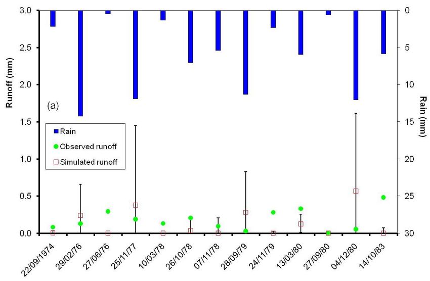
3.2 Calibration and validation fitted the observed events reasonably well. For the 17 vali-
dation events, the fit was not as good, an R 2 of 0.44 and an
The results of the base run indicated that for high rainfall E of 0.43 were obtained. The MAEs of the calibration and
events in the upstream areas runoff was generally underesti- validation periods were 2.6 and 3.0 mm, respectively.
mated by the model, whereas for events with high rainfall in The validation period clearly suffered from the absence of
the mid- and downstream areas runoff was overestimated. As the Koutine and Allamet rain gauges, which cover most of
FLOW OUT is most sensitive to the CN, adjustments were the downstream and midstream areas. In their absence, the
made to the CN as shown in Table 2. To reduce the runoff in rain was interpolated from the remaining four rain gauges
the mid- and downstream area, the CN of the cereals and the plus the Médenine station. The lack of rain gauges in the
rangelands in the plain was reduced. However, the reduction downstream area resulted in an underestimation of three of
of the CN is constrained by the shallowness of the major- the four runoff events observed during this period. The Kou-
ity of the soils covered by these land uses. These shallow tine gauge, which is located near the outlet, became opera-
soils fill up quickly, with the remainder of the rain turning in tional in September 1975 and the Allamet gauge in Septem-
to runoff, lateral flow and percolation. The mountain range- ber 1976. During the 1975–76 season, the rain over the lower
lands on the soils in the downstream areas (ISOH, PEAH) midstream area was covered by the downstream Koutine rain
were assumed to have similar CNs as the plain rangelands gauge, which resulted in the opposite effect, with five of the
on these soils. For the mountain rangelands on the shallow seven events overestimated.
soils (MBEH, CRCG), which are mainly found on the slop- It is important to note that 50% of the total runoff of the
ing lands in the upstream and midstream areas, the CN was 12-year period is produced by two events. The largest event,
increased by 2 points. Because the area occupied by jes- which occurred in March 1979 (calibration period), had an
sour seemed to be somewhat overestimated, the DIVMAX area-weighted rainfall of 166 mm over the watershed and an
of jessour was reduced from 0.25 to 0.22 m, which also in- observed runoff of 42 mm. This event was estimated quite
creased the runoff from the upstream areas. The FLOWFR well by the model (47 mm). The second largest event, on
of the tabias, which capture a large part of the runoff of the December 1973 (validation period), which received 91 mm
upstream areas, was reduced from 95 to 90%. rain and 30 mm runoff, was clearly underestimated (12 mm)
and the observed runoff did not even fall inside the bound-
The R 2 of the 21 calibrated runoff events was 0.77 and the
aries of the extreme parameter sets (Fig. 7). This was most
Nash-Sutcliffe coefficient was 0.73. A graphical representa-
likely at least partly due to absence of both the Koutine and
tion of the observed versus simulated outflow of the recorded
the Allamet rain gauges.
events at Koutine station is presented in Fig. 5. As can be
seen, the calibrated events (September 1978–August 1985)
www.hydrol-earth-syst-sci.net/13/2003/2009/ Hydrol. Earth Syst. Sci., 13, 2003–2021, 2009You can also read