Modifying emissions scenario projections to account for the effects of COVID-19: protocol for CovidMIP - GMD
←
→
Page content transcription
If your browser does not render page correctly, please read the page content below
Geosci. Model Dev., 14, 3683–3695, 2021
https://doi.org/10.5194/gmd-14-3683-2021
© Author(s) 2021. This work is distributed under
the Creative Commons Attribution 4.0 License.

Modifying emissions scenario projections to account for the effects
of COVID-19: protocol for CovidMIP
Robin D. Lamboll1 , Chris D. Jones2 , Ragnhild B. Skeie3 , Stephanie Fiedler4,5 , Bjørn H. Samset3 , Nathan P. Gillett6 ,
Joeri Rogelj1,7 , and Piers M. Forster8
1 Grantham    Institute for Climate Change and the Environment, Imperial College London, London, UK
2 Met  Office Hadley Centre, Exeter, UK
3 CICERO Center for International Climate Research, Oslo, Norway
4 Institute of Geophysics and Meteorology, University of Cologne, Cologne, Germany
5 Hans-Ertel-Centre for Weather Research, Climate Monitoring and Diagnostics, Bonn/Cologne, Germany
6 Canadian Centre for Climate Modelling and Analysis, Environment and Climate Change Canada, Victoria, Canada
7 International Institute for Applied Systems Analysis, Laxenburg, Austria
8 Priestley International Centre for Climate, University of Leeds, Leeds, UK

Correspondence: Robin D. Lamboll (r.lamboll@imperial.ac.uk) and Chris D. Jones (chris.d.jones@metoffice.gov.uk)

Received: 6 November 2020 – Discussion started: 10 December 2020
Revised: 4 May 2021 – Accepted: 19 May 2021 – Published: 22 June 2021

Abstract. Lockdowns to avoid the spread of COVID-19               also form part of the Detection and Attribution Model Inter-
have created an unprecedented reduction in human emis-            comparison Project (DAMIP).
sions. While the country-level scale of emissions changes
can be estimated in near real time, the more detailed, grid-
ded emissions estimates that are required to run general cir-
culation models (GCMs) of the climate will take longer to         1   Introduction
collect. In this paper we use recorded and projected country-
and-sector activity levels to modify gridded predictions from     Climate change research routinely uses emissions scenarios
the MESSAGE-GLOBIOM SSP2-4.5 scenario. We provide                 to explore potential future impacts of climate change. These
updated projections for concentrations of greenhouse gases,       scenarios are developed with integrated assessment models
emissions fields for aerosols, and precursors and the ozone       (IAMs) that project internally consistent evolutions of green-
and optical properties that result from this. The code base to    house gases based on socioeconomic and technological as-
perform similar modifications to other scenarios is also pro-     sumptions for the 21st century (Weyant, 2017; Riahi et al.,
vided.                                                            2017; Rogelj et al., 2018). Scenarios are projections, not pre-
   We outline the means by which these results may be             dictions, and by design reality will differ from the precise
used in a model intercomparison project (CovidMIP) to in-         evolutions contained in their description. However as we re-
vestigate the impact of national lockdown measures on cli-        ceive more information, the greenhouse gas emission path-
mate, including regional temperature, precipitation, and cir-     ways of IAM scenarios can be modified to more accurately
culation changes. This includes three strands: an assessment      reflect their historical evolution or societal changes. This pos-
of short-term effects (5-year period) and of longer-term ef-      sibility has gained acute interest in the context of the current
fects (30 years) and an investigation into the separate effects   COVID-19 pandemic.
of changes in emissions of greenhouse gases and aerosols.            Societal lockdown measures to contain the spread of
This last strand supports the possible attribution of observed    COVID-19 have resulted in unprecedented global changes
changes in the climate system; hence these simulations will       to the emissions of greenhouse gases (GHGs) and aerosols
                                                                  (Le Quéré et al., 2020a; Venter et al., 2020; Forster et al.,
                                                                  2020a). There are reports of a 36 % reduction in population-

Published by Copernicus Publications on behalf of the European Geosciences Union.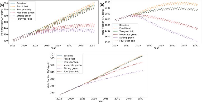
3684                          R. D. Lamboll et al.: Modifying emissions scenario projections for the effects of COVID-19

averaged global NO2 concentrations (Venter et al., 2020) for     government investment, towards either the fossil fuel econ-
34 countries prior to 15 May, and CO2 emissions are esti-        omy or green infrastructure, can have much longer-term im-
mated to have fallen by 4 %–8 % in 2020 (Le Quéré et al.,        pact (Gillingham et al., 2020; Andrijevic et al., 2020). We
2020b; IEA, 2020; Liu et al., 2020; Le Quéré et al., 2021).      therefore supplement the short-term emissions modifications
Shorter-duration and localised changes have been even more       with several possible global emissions trends. These diverge
extreme (Bauwens et al., 2020; Yang et al., 2020) but show       from each other only in the future, unlike the pre-existing
nonlinear changes in air chemistry that simple, globally aver-   SSP scenario sets (which diverge after 2015). This prevents
aged climate models will miss (Le et al., 2020). Estimates of    us ascribing any retrospective improvements to the effects of
the immediate impact of this change on global temperature        the pandemic.
have already been quantified as small using simple climate          We use this analysis to generate five scenarios of grid-
models (Forster et al., 2020a), but these models do not cap-     ded emissions and concentrations incorporating the effects
ture complex chemistry, regional temperatures, or precipita-     of lockdown and various different recoveries. We also pro-
tion effects with any confidence, which are also more uncer-     cess the emissions fields through an atmospheric chemistry
tain and sensitive to small changes. The unexpected changes      model to provide the ozone field, often required as an input
in emissions are potentially enough to raise questions about     for general circulation models (GCMs). We finally describe
the relevance of projections made only years before. Existing    a protocol for a model intercomparison project (MIP) assess-
gridded emissions scenarios are too poorly designed to even      ing the impact of national lockdown measures. Based on dis-
represent realistic emissions changes on less than a 10-year     cussions between several modelling groups, this activity aims
basis.                                                           to establish the scope of changes in climate results to be ex-
   It is therefore desirable to explore the impact of these      pected from the direct impacts of lockdown and the potential
changes on climate change projections, both to establish to      impact of changes to investment structure resulting from the
what extent simulations ignoring the effects so far need up-     recovery packages. Since the changes being investigated are
dating due to short-term changes and to investigate poten-       likely rather small, the use of a common protocol for mod-
tial impacts of the lockdown in the long term. This is chal-     elling groups to perform makes both optimal use of the effort
lenging because country-level emissions estimates are often      to produce the emissions data and also increases the ability
generated only on a yearly basis, missing the variations be-     to make a robust assessment of the results. We emphasise the
tween months or weeks. Moreover, detailed climate simu-          importance of both as an initial condition ensemble as possi-
lations require emission statistics to be broken down on a       ble, and we also use of “nudging” techniques for improving
higher-resolution uniform grid, and these are typically only     the signal-to-noise ratio and for establishing a sufficient body
estimated several years after the emissions have occurred        of simulations for the different parts of the MIP.
(Feng et al., 2020; Meinshausen et al., 2020).
   This paper uses data from near-simultaneous “nowcast-
ing” methods based on open-access data on mobility, energy       2   Data sources
grids, and aviation to modify a pre-existing gridded projec-
tion by country- and sector-specific factors. By expressing      For this exercise, we change the concentration of the three
our scenario as a modification of a pre-existing scenario, we    main greenhouse gases (GHGs) – CO2 , CH4 , and N2 O – and
have an estimation of sector emissions on a grid that simu-      emissions of the main aerosols and aerosol and ozone pre-
lation teams know how to handle. We can also use the pre-        cursors: black carbon (BC), CO, NH3 , non-methane volatile
existing runs of the baseline scenario as our point of compar-   organic compounds (NMVOCs) as an aggregate, NOx , or-
ison and to provide the initialisation condition for the mod-    ganic carbon (OC), and SO2 . For aviation emissions, only
ified run. This reduces the computational load of running a      changes in CO2 and NOx are modelled. Other emissions
complete new model when rapid results are desired.               (such as HFCs) are assumed not to change from their base-
   The country-level analysis of Forster et al. (2020a) pro-     line behaviour, since either no change in these emissions is
vided a means to assess the level of lockdown affecting dif-     expected or the total impact of these emissions on the climate
ferent sectors. It used sector-specific changes in Google mo-    is so small that a small change in the emissions is likely to
bility data, supplemented by an analysis of the legally im-      have negligible effects.
posed degree of confinement from Le Quéré et al. (2020a), to        The baseline dataset for our analysis is the MESSAGE-
produce an up-to-date assessment of the emissions changes        GLOBIOM model SSP2-4.5 (Fricko et al., 2017), taken from
in 142 countries. We use updated data following the same         the gridded CMIP6 data Input4MIPs (Feng et al., 2020). This
technique and add a new methodology for aviation data, then      choice is made for several reasons. Firstly, it is a CMIP6
use this to estimate the short-term impact on emissions from     ScenarioMIP tier 1 scenario, meaning that all groups in-
COVID-19. The impact of lockdown itself on emissions is          volved in CMIP6 ScenarioMIP have run the baseline sce-
likely to be only short-term, since most financial crashes to    nario O’Neill et al. (2016). Of these, it is the most middle-
date have provided only a temporary fall in annual emissions     of-the-road in terms of assumptions, both about future polit-
(Le Quéré et al., 2021). However the impact of changes in        ical and economic developments, because it is SSP2 (Riahi

Geosci. Model Dev., 14, 3683–3695, 2021                                          https://doi.org/10.5194/gmd-14-3683-2021
R. D. Lamboll et al.: Modifying emissions scenario projections for the effects of COVID-19                                    3685

et al., 2017) and because it has intermediate long-term forc-      3     Concentration data
ing (4.5 W m−2 ). This amount of forcing is consistent with
the global level of warming implied by countries’ current          Most GCMs use global or hemispherically averaged lev-
nationally determined contribution (NDC) pledges (Climate          els for well-mixed GHGs. These were directly calculated
Action Tracker, 2021) and has projected values closest to the      in Forster et al. (2020a) using the FaIR v1.5 reduced-
most recently measured emissions (Pedersen et al., 2021).          complexity climate model (Smith et al., 2018). To make this
SSP2-4.5 is also used in decadal predictions and is therefore      consistent with the general emissions trends found in SSP2-
of relevance to near-term climate forecasts. We emphasise          4.5, we calculate the ratio of the concentrations between the
that the code that generates the data that follows can be ap-      baseline and the specific COVID-19 scenarios in the Forster
plied to other scenarios as well.                                  data and apply that multiplier to the global and hemispheric
   This baseline scenario is then modified to match                trends in the SSP2-4.5 data to produce the corresponding
the country-and-sector-specific emissions or concentration         concentration trends.
trends supplied using the methodology of Forster et al.               A few GCM models use CO2 emissions data, which they
(2020a) for times after 2020, updated where such data are          put through their own carbon cycle representation. These
available. This technique projects the emissions change for        data are available as described in the “Emissions data” sec-
the most recently measured month to continue at two-thirds         tion below. We remark that the results of the two approaches
of its value, in most scenarios until the end of 2021. In the      do not necessarily coincide, since the emissions in Forster
4-year blip scenario we continue this until the end of 2023.       et al. (2020a) differ from the emissions in this paper in three
In all scenarios we then expect recovery back to the base-         ways. Firstly, the baseline country emissions in 2020 are
line over the following year. This is not necessarily the time     based on more recent data than the baseline in SSP2-4.5. Sec-
for the virus to have been completely eliminated or habitu-        ondly, Forster et al. (2020a) use aviation data based on the Le
ated to but merely the time for countries to no longer con-        Quéré et al. (2020a) rather than on more recent Flightradar24
sider lockdowns an effective intervention. After that, we no       data. Thirdly, Forster et al. (2020a) assume that CO2 emis-
longer make country-specific modifications but instead mod-        sions from agriculture, forestry, and other land use (AFOLU)
ify global emissions by a constant factor, indicating four dif-    are reduced by the same amount as the average CO2 emis-
ferent styles of recovery from lockdown to have either no          sions change from industry, whereas here we assume no dif-
difference from the baseline (the “2-year blip” and “4-year        ference in AFOLU emissions. This is due to the finding that
blip” scenarios), a transition to an increased use of fossil fu-   global deforestation has not slowed down due to lockdown
els (“fossil fuel development”), or either moderate or large-      (Saavedra, 2020; Daly, 2020), and we expect that agricultural
scale increases in the investment in a green recovery (“mod-       output will remain broadly consistent with pre-lockdown lev-
erate green” and “strong green”). The nature of these sce-         els.
narios is summarised in Table 2 and most are described in
Forster et al. (2020a), although the 4-year blip is new here.
The impact of these paths is felt on different emissions to a      4     Emissions data
different extent (and often with a different sign, for instance
greener scenarios emit more NH3 but less SO2 ), but we do          4.1    Interpolating additional times
not break down this effect by sector.
   As discussed in Forster et al. (2020a), data are not avail-     Many gridded IAM models do not report emissions monthly
able for several regions and sectors, notably including China      but only on a 5- or 10-year average basis, and climate models
and all aviation and shipping. In these instances, emissions       simply interpolate these data for the remaining years. Typi-
modifications are taken instead from Le Quéré et al. (2020a),      cally, emissions changes are smooth and the amount of data
except for aviation emissions, which are instead modified us-      lost in this way is therefore low. However, when a particu-
ing data obtained from Flightradar24 (2021).                       larly strong trend occurs suddenly this is difficult to represent
   A minor complication of combining these data sources is         on this timescale. Because 2020 is a year normally reported
that the SSP2-4.5 data use 365 d years, whereas we also have       by IAMs, if the emissions for this year were simply corrected
real data from the leap day in February 2020. To ensure com-       without changing anything else, then the effects of lockdown
patibility with climate models, data from the leap day are in-     would also be felt in the interpolated years before it started as
corporated into the monthly averages but the output file will      well as in following years when it is expected to have ended.
not include a day for it.                                          It is therefore necessary to interpolate additional years into
   As this was an evolving project with different amounts of       all datasets with lockdown effects in them – we interpolate
data available at different stages, several versions of the data   2019, 2021, and 2023. We require data for 2019 to ensure no
were released. The details of the code changes involved can        emissions reduction in the years before lockdown starts. We
be found in Table 1.                                               similarly interpolate 2023 before modifications are made to
                                                                   ensure long-term effects only happen when the model dic-
                                                                   tates. Since the years 2020 and 2021 are expected to be very

https://doi.org/10.5194/gmd-14-3683-2021                                             Geosci. Model Dev., 14, 3683–3695, 2021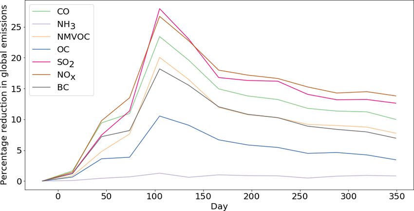
3686                             R. D. Lamboll et al.: Modifying emissions scenario projections for the effects of COVID-19

Table 1. Table of noteworthy difference between versions of data. The first digit of the version number is incremented by both additional
months of complete data and by major coding developments. The second digit represents significant coding changes or additional data use
within the same final month of data – these data are broadly inter-compatible. The third decimal place denotes changes in the times at which
data are reported or minor bug fixes.

           Version no.        Data date           Notes
           1.0                14/05/2020          First available data
           3.0                17/06/2020          Major bug fix – data before this point should not be used
           4.0                14/07/2020          Pixels whose four corners are in the sea use internationally averaged shipping
                                                  factors
           5.0                25/01/2020          Substantial update of data to cover 2020; bug fix affecting aerosol values on
                                                  December 2021

Table 2. Summary table for the differences between scenarios. For more details on how these were constructed, see Forster et al. (2020a).
More details on the calculation of the emissions values themselves can be found in the file “InfillingCovidResponse.ipynb” in Lamboll
(2020a).

   Scenario              Assumptions
   Baseline              SSP 2-4.5 data are used without modification.
   Two-year blip         Data are modified for all of 2020 and 2021 in accordance with observed activity levels in the sectors of different
                         countries. This is projected to continue at two-thirds of the activity reduction value for the latest month available
                         for the rest of the 2-year period. Activity is interpolated, month for month, back towards the baseline over 2022
                         and is equal to the baseline thereafter.
   Four-year blip        As for 2-year blip, except the projected activity reduction, of two-thirds of the last month available, is continued
                         until 2023. Activity is interpolated, month for month, back towards the baseline over 2024 and is equal to the
                         baseline thereafter.
   Fossil fuel           Follows 2-year blip until 2023. Thereafter, the effects of additional investment in fossil fuels during recovery are
                         included in a globally uniform way. Financial modelling produced estimated global Kyoto gas emissions totals
                         consistent with 10 % higher emissions than the path met if countries meet their nationally determined contribu-
                         tions (NDCs). We used the open-source package Silicone (Lamboll et al., 2020a) to find a linear combination
                         of MESSAGE-GLOBIOM SSP2 scenarios that gave the same total Kyoto emissions. We use the global relative
                         emissions level of each aerosol and precursor in this composite scenario to rescale the 2D emissions maps. The
                         relative concentration change arising from this scenario is used to rescale global greenhouse gas concentrations.
   Moderate green        Follows 2-year blip until 2023. Thereafter, the effects of small additional investment in green technology are
                         included in a globally uniform way. Financial considerations as to what emissions change is plausible with
                         moderate ambition (in keeping with results in McCollum et al., 2018) produced a Kyoto emissions total in
                         2030 of 35 % lower than the NDCs, which we resolve into a linear combination of MESSAGE-GLOBIOM
                         SSP2 scenarios. We then set a global net-zero CO2 trajectory for 2060 and resolve this CO2 total into a linear
                         combination of MESSAGE-GLOBIOM SSP2 scenarios again using Silicone. The relative difference between
                         this scenario and the baseline is used to rescale emissions and concentrations as in the fossil fuel case.
   Strong green          Follows 2-year blip until 2023. Thereafter, the effects of large additional investment in green technology are
                         assumed to push the scenario towards an IMAGE SSP1 world. In 2030 we are assumed to reach the emissions
                         rate of SSP1-19, around 52 % lower than following current NDCs, and thereafter follow a global net-zero CO2
                         target for 2050. The other emissions are formed by a linear combination of IMAGE SSP1 scenarios that give
                         the closest total CO2 match to this pathway. (This composite pathway is always close to the SSP1-19 pathway
                         after 2023.)

different from the surrounding years, they are both interpo-               here. By request from certain groups, monthly data with ev-
lated and modified by the effects of lockdown. The year 2022               ery year from 2015 to 2025 are available, as are weekly data
is defined as exactly equalling the value interpolated, month              for 2020 used by Gettelman et al. (2020). Since emissions
for month, between the effects of lockdown and the base-                   change on a seasonal basis, interpolated years are interpo-
line behaviour. This is the normal default infilling method of             lated between the same months of the years with available
climate simulators, so explicit values are not usually needed

Geosci. Model Dev., 14, 3683–3695, 2021                                                      https://doi.org/10.5194/gmd-14-3683-2021
R. D. Lamboll et al.: Modifying emissions scenario projections for the effects of COVID-19 3687
data on either side. This is done before imposing the effects in the emissions modification GitHub repository, stored in
of lockdown, except when we add data for 2022. Zenodo; see “Code availability” section.
4.3 Aviation emissions – monthly, versions up to 4
4.2 Relative emissions factors
The aviation activity level is always treated globally. The
The process for handling emissions is more complicated than daily number of flights is taken from Flightradar24 free data.
concentrations and was subject to a significant change be- This is available from 6 January 2020 up to the time the ver-
tween version 3 and version 4 for shipping. The different sion is defined. The “null flights” level is calculated as the av-
versions are described in Table 1. erage number of flights per day in January, and activity level
The baseline SSP2-4.5 data contain emissions for nine is then expressed as the daily number of flights divided by
sectors: AFOLU; energy; industrial processes; surface trans- this. After the end of the available data, we project a linear
portation; residential, commercial, and other; solvent pro- trend, fitted to data collected after 1 May 2020 (not inclu-
duction and application; waste; international shipping; and sive), until it reaches the long-term level. This is defined as
aviation. Aviation emissions are subdivided by altitude and two-thirds of the reduction factor of the last complete month
handled separately. These mostly map well onto the sec- of data. In equation form, with angular brackets indicating
tors whose activity levels were investigated by Forster et al. the mean over the subscript period, f (t) representing flights
(2020a), with two exceptions. Firstly Forster et al. (2020a) on the date t days past 1 January and a(t) representing activ-
model residential and public/commercial buildings sepa- ity level, f0 = hf iJan and
rately, so we will use the emissions-weighted mean of these (
for each country. Secondly, Forster et al. (2020a) did not f (t)/f0 if data exists
have sector-specific estimates for emissions changes from a(t) =
2
min mt + c, 1 − 3 hailatest month otherwise
solvents, waste, or AFOLU (although CO2 emissions from
AFOLU are implicitly assumed to scale with the industrial (1)
emissions reduction, as discussed above). We will assume
that no changes occurred to these sectors. This is because for constants m and c that are fit to the data from dates after
we do not expect these sectors to be directly affected by 1 May 2020. For some versions of the data, the flight activity
lockdown, and the reductions in the general economic level level is already at the two-thirds reduction level by the end of
will be partly offset by a reduction in regulatory oversight, the period of collected data so no linear interpolation is seen.
as has been documented in deforestation changes (Saavedra, The monthly average of these data is then taken to produce
2020; Daly, 2020). We similarly assume that the small is- the activity level of aviation. This is assumed to be globally
land nations and regions like Antarctica not included in the uniform and the same across all altitudes. See the graphical
143 nations estimated by Forster et al. (2020a) experience no illustration in Fig. 4a.
change in emissions, for convenience.
4.4 Aviation emissions – weekly or version 5
Emissions in the SSP2-4.5 data are broken down by lati-
tude and longitude, so we must classify each emissions pixel Most analyses do not use any higher resolution than monthly,
as belonging to a single country. We assign each pixel using but for one project (Gettelman et al., 2020), weekly data are
the reverse_geocoder python module (Thampi, 2015) to the investigated for the 2020 data. For this project, using open-
centre of the pixel, which identifies the country that pixel be- source data was not required, so we obtained previous years
longs to. It assigns areas of sea to the nearest country. We of flight data from FlightRadar24 to better control for sea-
then check whether the four corners of the pixel are all in sonal changes. We can then use the weekly-averaged data
the sea using the global_land_mask python module (Karin, from 2018 and 2019 for the corresponding day as the base-
2020). If all four corners are sea, the pixel is instead classi- line instead of the January values:
fied as international waters and is therefore modified by the
internationally averaged change in shipping activity rather 2 hf2020 (j )ij =t:t+7
than the national change in shipping level. Using this defini- a(t) = , (2)
hf2018 (j ) + f2019 (j )ij =t:t+7
tion, only shipping emissions are found in international wa-
ters. We emphasise that this classification scheme is purely where the subscript on the f indicates the year the flight data
for emissions calculations and should not be interpreted as a are taken from. This produces a weekly-averaged rather than
statement of political designation. This treatment of the seas actual daily factor, since it is not possible to decouple sea-
began in version 4 – prior to this, all sea activity used the sonal/holiday and weekday effects. Using weekly averages
national shipping activity level of the closest country. Exam- both removes the weekday effects and reduces the intrinsic
ples of this analysis for April can be found in Fig. 2, and the variability in the data. This analysis reveals that there are sig-
globally averaged emissions reduction factors can be found nificant seasonal effects and implies that later versions of the
in Fig. 3. An animation of the global distribution is available code should also attempt to correct for this – see Fig. 4b.
https://doi.org/10.5194/gmd-14-3683-2021 Geosci. Model Dev., 14, 3683–3695, 20213688 R. D. Lamboll et al.: Modifying emissions scenario projections for the effects of COVID-19
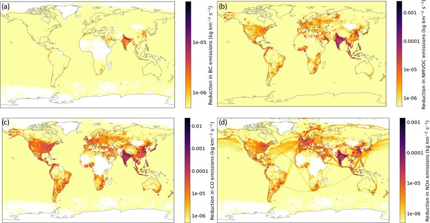
Figure 1. Concentrations for the three persistent GHGs: (a) CO2 , (b) CH4 , and (c) N2 O. In each case the baseline data are very similar to 2-
and 4-year blips, hence the difficulty distinguishing between the lines.
Figure 2. Difference in emissions between the baseline and the 2-year blip COVID-19 scenario during April 2020. White regions indicate
that the emissions change was zero (often due to emissions being zero in the first place) or emissions increased. Species are (a) BC, (b)
NMVOC, (c) CO, and (d) NOx .
After the end of the data, we use a linear trend to reach to the output with recent results but required the introduction
two-thirds of the last month’s average factor as before. As of new parameters to define where the linear trend began.
of 8 October 2020, the data for 2019 have also been released
open-source, so for version 5 of the data and onwards this ap-
proach (with either weekly or monthly averaging) is used for 5 Data for aerosol optical properties and associated
all outputs. We also stop the linear interpolation to the base- effects on clouds
line for monthly behaviour, since this made little difference
Data for the anthropogenic aerosol optical properties and an
associated effect on clouds are available via the MACv2-
Geosci. Model Dev., 14, 3683–3695, 2021 https://doi.org/10.5194/gmd-14-3683-2021R. D. Lamboll et al.: Modifying emissions scenario projections for the effects of COVID-19 3689
by following the method previously applied to other gridded
emissions data from CMIP6 (Fiedler et al., 2019a). The re-
sults for the anthropogenic aerosol optical depth, τa , point
to a global decrease by 10 % due to the pandemic in 2020
relative to the baseline. First estimates of the effective radia-
tive forcing associated with anthropogenic aerosols in 2020
point to a less negative global mean by +0.04 W m−2 relative
to the baseline. Such small effective radiative forcing (ERF)
differences are difficult to determine due to the large impact
of model-internal variability (e.g. Fiedler et al., 2019b). We
therefore propose to run ensembles of simulations for partic-
Figure 3. Monthly global emissions reduction estimates for 2020 in ipating in CovidMIP. The post-pandemic recovery of emis-
version 5 of the data. sions is associated with a global τa increase in two out of four
scenarios until 2030 and reductions in all scenarios there-
after (Fiedler et al., 2021). In 2050, the τa spread is 0.012
to 0.02. This is a decrease in τa relative to 2005 and rela-
tive to four out of nine of the original CMIP6 scenarios for
2050 (Fiedler et al., 2019a). Using the new MACV2-SP data
in EC-Earth3 suggests an associated ERF spread of −0.38 to
−0.68 W m−2 for 2050 relative to the pre-industrial period,
which falls within the present-day uncertainty of aerosol ra-
diative forcing (Fiedler et al., 2021).
6 Ozone data
For models without ozone chemistry schemes, ozone fields
are generated using the OsloCTM3 model (Søvde et al.,
2012; Skeie et al., 2020). The OsloCTM3 is a chemistry
transport model driven by 3-hourly meteorological fore-
cast data by the Open Integrated Forecast System (Open
IFS, cycle 38 revision 1) at the European Centre for
Medium-Range Weather Forecasts. The horizontal resolution
is ∼ 2.25◦ × 2.25◦ with 60 vertical layers ranging from the
surface up to 0.1 hPa. Here, the meteorological data for the
Figure 4. Aviation data for (a) monthly calculation of activity level year 2014 are used in the simulations.
– this is normalised to the January data, as data from previous years The emissions fields described in Sect. 4 are used as input
were not available in open-source format – and (b) workings to- to the model as monthly fields. Natural emissions including
wards weekly activity level, using closed-source data from previ- biomass burning emissions are kept constant, and the ozone-
ous years too. This approach is used from version 5 onwards for depleting substances are kept the same in all simulations. The
monthly data too. surface methane concentrations are scaled by the increase in
concentration since 2019 provided in Sect. 3.
Time slice simulations for the years 2020, 2021, 2023,
SP parameterisation (Fiedler et al., 2017; Stevens et al., 2030, 2040, and 2050 are performed using emissions from
2017). Models using MACv2-SP can obtain the necessary the four scenarios as well as the baseline scenario SSP2-4.5
input data from the supplementary material of Fiedler et al. (Feng et al., 2020). The ozone in the 2-year blip scenario is
(2021) for participating in the model intercomparison project equal to that in the other scenarios for 2020 and 2021 and
(CovidMIP) experiments. A detailed assessment of the new equal to that of the baseline simulation for the remaining
MACv2-SP data suggests that the global aerosol radiative years. The changes in ozone in the 2-year blip compared to
forcing from CovidMIP will fall within the original spread the baseline scenario are shown in Fig. 5a for April 2020
in the CMIP6 scenarios (Fiedler et al., 2021). with a decrease of up to 6 % in the Northern Hemisphere
All scenarios from Forster et al. (2020a) have been used troposphere. Figure 5b shows the change in total ozone in
to create consistent MACv2-SP data (Fiedler et al., 2021). the different scenarios from 2019 and up to 2050 from the
To this end, annual scaling factors for MACv2-SP have been OsloCTM3 simulations relative to the baseline. For 2020 and
calculated from the SO2 and NH3 emissions from all sectors 2021 the total ozone decreased by 1 Dobson unit (DU) in the
https://doi.org/10.5194/gmd-14-3683-2021 Geosci. Model Dev., 14, 3683–3695, 20213690 R. D. Lamboll et al.: Modifying emissions scenario projections for the effects of COVID-19
2-year blip compared to the baseline. In 2023 all scenarios year blip forcing. This will be an initial condition ensemble,
are similar. For the fossil fuel scenario, the ozone changes are with model-by-model choice how to arrive at perturbed ini-
positive relative to the baseline scenario but less than 1 DU. tial conditions. Note the requirement that parallel SSP2-4.5
The largest change in ozone is for the strong green scenario, simulations already exist, so we anticipate that the same en-
with a decrease of 6 DU in 2050 compared to the baseline semble technique and initial conditions can be used.
scenario. Protocol details can be found in Table 3.
The modelled absolute difference in ozone between the
scenario and the baseline are added to the CCMI SSP2-4.5 7.2 Strand-2: longer-term impact of recovery scenarios
v1.0 ozone dataset prepared for input4MIPs (Hegglin et al.,
2020). The absolute ozone changes are horizontally and ver- This strand uses the three recovery scenarios derived by
tically interpolated to the same grid as the input4MIPs fields, Forster et al. (2020a): strong and moderate green stimulus re-
and the monthly mean values are linearly interpolated for the covery and a fossil-fuel rebound economic recovery scenario.
years in between the years simulated. We place the highest priority (tier 1) on the strong green stim-
ulus recovery as it will likely have the highest signal. As ex-
pansion work (tier 3), it includes the short-term lockdown
impacts (2-year and 4-year blip scenarios). The experiments
7 Protocol for CovidMIP
are tabulated in Table 3. For full details of the scenarios, see
Forster et al. (2020a), but results are summarised in Table 2.
The emissions and concentrations described above are used
in CMIP6 Earth system models to simulate the climatic im- 7.3 Strand-3: separation of forcing
pacts of lockdown. There are three focuses or strands to this
MIP. The first is to address the short-term response to the COVID lockdown has led to reduced emissions across a wide
emissions reductions, and the second is to address the longer- range of sectors and species. Some of these have compet-
term response to alternative recovery scenarios. There are ing or offsetting effects on atmospheric composition, radia-
sufficient differences in design and groups interested to make tive forcing, and climate. For example, Forster et al. (2020a)
this split pragmatic. The third focus is on understanding pro- show that at a global level the near-term warming due to re-
cesses and separating out the role of individual forcing com- duced aerosols may be at least partially offset by reduced
ponents in contributing to changes in radiative forcing and greenhouse forcing from ozone. Only on longer timescales
climate. does the climate effect of CO2 reductions become significant.
Some model groups also have the ability to perform In this strand we use both detection and attribution tech-
“nudged” simulations which force their model’s physical niques and fixed-SST (sea-surface temperature) diagnosis
state towards a pre-defined meteorology. This can reduce techniques to isolate and compare the ERF from individual
signal-to-noise issues and help identify aspects of atmo- emission types or categories and their full implications for
spheric composition which might not be apparent in “free- regional and global climate evolution.
running” model simulations. This is preferred where models Two detection and attribution simulations are proposed to
have this capacity. parallel ssp245-covid and allow the separation of the effects
It is assumed that model groups have performed the SSP2- of aerosols and well-mixed greenhouse gas perturbations on
4.5 scenario simulations, and we use this as a reference set of climate, similar to the way that hist-aer and hist-GHG sim-
simulations (baseline) against which we will compare Covid- ulations in DAMIP allow the separation of the effects of
MIP results. Any forcing or aspect of simulation not explic- these forcings over the full historical period (Gillett et al.,
itly defined in this protocol (for example HFCs or land +use) 2016). The ssp245-cov-aer simulation is identical to ssp245-
should be kept unchanged from the SSP2-4.5 simulation. covid, except that only aerosol and aerosol precursor emis-
sions (BC, OC, SO2 , SO4 , NOx , NH3 , CO, NMVOCs) follow
7.1 Strand-1: near-term impact of COVID-lockdown ssp245-covid, while greenhouse gas concentrations, ozone,
emissions reductions and all other forcings follow ssp245. Similarly the ssp245-
cov-GHG simulation is identical to ssp245-covid, except that
The goal of these simulations is to assess the impact of only the concentrations of the well-mixed greenhouse gases
COVID-induced lockdown emissions reductions on climate, follow ssp245-covid, while all other forcings follow ssp245.
atmospheric composition, and air quality in the near term. To We suggest that groups run as large ensembles of these sim-
achieve this, we use emissions reductions as close as possi- ulations as possible, but no minimum size is required.
ble to real emissions as reconstructed from activity data de-
scribed above. A recovery to baseline emissions is assumed 7.3.1 ERF calculations
by either (for the tier 1 emissions case) 2023 or (tier 2) 2025,
and simulations should run for 5 years (although longer is The most commonly used methodology for estimating ERF
also accepted – see Sect. 6.2). For the tier 1 case, we use is to utilise simulations with fixed sea-surface temperatures
the 2-year blip forcing, and for the tier 2 case we use the 4- (fSST) and prescribed emissions (Richardson et al., 2019;
Geosci. Model Dev., 14, 3683–3695, 2021 https://doi.org/10.5194/gmd-14-3683-2021R. D. Lamboll et al.: Modifying emissions scenario projections for the effects of COVID-19 3691 Figure 5. (a) The relative difference in ozone zonal concentration between the 2-year blip and the baseline in April 2020 (%) in the OsloCTM3. The vertical coordinates in OsloCTM3 are hybrid sigma–pressure levels. The field is plotted for the model levels and indi- cated by approximate pressure levels on the y axis. (b) The difference in annual total ozone (DU) between the scenarios and the baseline simulations in the OsloCTM3. Table 3. Table of experiments for CovidMIP. All experiments branch from SSP2-4.5 on 1 January 2020. Emissions/concentrations not specified come from the baseline data. Strand Name Tier Run length Recommended ensemble size scenarios 1 ssp245-covid 1 5 years or more As large as possible, 10+ members 2-year blip 1 ssp245-covid4yr 2 5 years or more As large as possible, 10+ members 4-year blip 2 ssp245-cov-strgreen 1 31 years 10 members Strong green 2 ssp245-cov-modgreen 2 31 years 10 members Moderate green 2 ssp245-cov-fossil 2 31 years 10 members Fossil fuel 2 ssp245-cov-2yr 3 31 years 10 members 2-year blip 2 ssp245-cov-4yr 3 31 years 10 members 4-year blip 3 ssp245-cov-aer 1 5 years or more As large as possible, 10+ members 2-year blip for aerosols 3 ssp245-cov-GHG 1 5 years or more As large as possible, 10+ members 2-year blip for GHGs 3 ssp245-cov-fsst 1 52 years As large as possible, 10+ members All baseline 3 ssp245-cov-fsst-aer 1 52 years As large as possible, 10+ members 2-year blip for SOx , BC, and OC 3 ssp245-cov-fsst-ozone 1 52 years As large as possible, 10+ members 2-year blip for NOx , CO, and NMVOC 3 ssp245-cov-fsst-bc 2 52 years As large as possible, 10+ members 2-year blip for BC 3 ssp245-cov-fsst-sox 2 52 years As large as possible, 10+ members 2-year blip for SOx 3 ssp245-cov-fsst-oc 2 52 years As large as possible, 10+ members 2-year blip for OC Pincus et al., 2016; Myhre et al., 2013). This allows the at- (CO2 , CH4 , N2 O) for all years. For the SST pattern, we pre- mospheric conditions to rapidly equilibrate, and rapid ad- fer repeated year 2021 values, taken from a coupled simu- justments to play out, but broadly avoid the feedbacks as- lation, but if this is challenging then another recent year is sociated with a change in surface temperature. For example, acceptable so long as the baseline and signal have the same Forster et al. (2016) found 30 years of fSST simulations suf- SSTs. Meteorology can vary according to internal variability ficient to reduce the global 5 %–95 % confidence interval to but should be representative of the year 2021. 0.1 W m−2 , superior to other methods. CovidMIP defines simulations for diagnosing ERF as fol- As CovidMIP aims to quantify ERFs that are likely to be lows. For tier 1, to quantify the forcing from aerosols and relatively weak, on the order of 0.01–0.1 W m−2 , the recom- ozone, we request mended protocol is to run 52-year simulations, where the first 2 years are spinup and the last 50 years are used for analysis. – ssp245-cov-fsst: all emissions from the baseline, year Quantification requires a baseline simulation and one dedi- 2021; cated simulation for each component to be quantified. Emis- sions are taken from the year 2021 of the “baseline” and 2- – ssp245-cov-fsst-aer: aerosol emissions (SOx , BC, OC) year blip scenarios from Forster et al. (2020a). For GHG con- from the 2-year blip and all other emissions from the centrations, we use the prescribed value for 1 January 2021 baseline; https://doi.org/10.5194/gmd-14-3683-2021 Geosci. Model Dev., 14, 3683–3695, 2021
3692                           R. D. Lamboll et al.: Modifying emissions scenario projections for the effects of COVID-19

  – ssp245-cov-fsst-ozone: ozone precursor emissions               gories of particulate matter (PMs). This will allow us to esti-
    (NOx , CO, NMVOC) from the 2-year blip and all other           mate the global impact of lockdown on health effects.
    emissions from the baseline.                                      Model data will be made freely available via the Earth Sys-
   For tier 2, to quantify the forcing from individual aerosol     tem Grid Federation (ESGF). Users of these data are encour-
species, we request runs with only a single emission species       aged to contact model group representatives and invite pos-
different from the baseline value. The three species for which     sible involvement in any resulting publications.
we want these experiments run are BC, SOx , and OC emis-              We expect this MIP will allow us to estimate the continued
sions from the 2-year blip. More details can be found in Ta-       relevance of climate projections that do not include the ef-
ble 3.                                                             fects of lockdown. If results significantly deviate from base-
   For all strands, we request that model groups produce the       line projections, then the continued relevance of outdated
same diagnostics as per their baseline SSP2-4.5 simulations,       simulations is questioned; if results are broadly similar, old
reported for the ScenarioMIP.                                      projections can be used with more confidence. Initial results
   As an alternative to fSST-based ERF diagnosis, some             indicate that the latter is the case.
models are able to run nudged simulations where meteo-
rological conditions (typically surface winds and temper-
                                                                   8    Conclusions
atures) are forced to be comparable between signal and
baseline. This allows for a direct, time-evolving calculation
                                                                   We have demonstrated a novel way to combine data-rich
of ERF based on differences in top-of-atmosphere radia-
                                                                   emissions nowcasting with long-term emissions projections
tive imbalance between the simulations (Chen and Gettel-
                                                                   to create a dataset suitable for investigating the impact of the
man, 2016; Liu et al., 2018). Although they may not cap-
                                                                   large and unforeseen emissions reduction arising from lock-
ture the full range of atmospheric adjustments (Forster et al.,
                                                                   down. This will form the basis for a model intercomparison
2016), nudged ERF calculations are sufficiently comparable
                                                                   project to answer questions around how much climatic im-
to fSST-based calculations that they will be used in Covid-
                                                                   pact we expect to observe from lockdown measures in both
MIP provided they have prescribed the same emissions as
                                                                   the short and medium term. We also provide ozone fields
described above.
                                                                   derived from these results for models that do not produce
7.4    Anticipated analysis                                        their own estimates of this. Finally we provide a protocol
                                                                   for how different simulation groups can run experiments on
CovidMIP analysis will primarily start with analysis of 2-         un-initialised, coupled atmosphere–ocean general circulation
year blip simulations up to 2025. The focus will be on main        model (AOGCMs)/ESMs.
climate outputs of surface temperature and rainfall, winds,
and basic circulation and also basic-level biogeochemical di-
agnostics such as carbon stores and fluxes. The first instance     Code availability. The code to perform this analysis and
of results are available at Jones et al. (2021). These show that   to generate an animation of the data is available at
                                                                   https://doi.org/10.5281/zenodo.4736578 (Lamboll, 2021).
the reduction in aerosols is clear in the 2020–2025 period,
                                                                      Old versions of the code and variants can be found at https:
but the impact of this on temperature or precipitation does
                                                                   //github.com/Rlamboll/modify_COVID19_netCDF_Emissions
not have a clear enough signal to be detectable in the aggre-      (Lamboll, 2020b).
gated data. Some individual models have found clearer trends
using nudged analysis (Gettelman et al., 2020).
   Similar analysis is planned but focusing on temperature         Data availability. The output of these protocols is available from
and precipitation extremes, with analysis based on maximum         several Zenodo addresses. Each address carries the different itera-
daily air temperature (tasmax) and precipitation data and a        tions of the same data where multiple versions are available.
focus on regional aspects. Regionally specific analyses are
                                                                       – The main set of monthly aerosols emissions and GHG con-
possible, with East Asia a particular focus region as this is
                                                                         centrations: https://doi.org/10.5281/zenodo.3957826 (Forster
where the largest effects of emissions have been seen in sur-            et al., 2020b);
face aerosols and air quality. The implications of this on local
rainfall and monsoon circulation patterns is of particular in-         – Four-year blip files for version 4 of the data:
terest. North Atlantic and European circulation changes will             https://doi.org/10.5281/zenodo.4446200 (Lamboll et al.,
                                                                         2021);
also be investigated.
   The effect of emissions reductions on CO2 concentrations            – CO2 emissions data, monthly, with data every year 2015–
is also of interest and may be investigated by Earth system              2025: https://doi.org/10.5281/zenodo.3951601 (Lamboll et al.,
models (ESMs) with the capability of performing emissions-               2020b);
driven CO2 simulations. Similarly, ESMs with atmospheric               – Aerosol       emissions     data,   daily  for            2020:
chemistry schemes will be investigated to see the role of                https://doi.org/10.5281/zenodo.3952960 (Lamboll      et     al.,
emissions reductions on surface ozone and different cate-                2020c);

Geosci. Model Dev., 14, 3683–3695, 2021                                               https://doi.org/10.5194/gmd-14-3683-2021
R. D. Lamboll et al.: Modifying emissions scenario projections for the effects of COVID-19 3693
– NOx emissions from aviation, weekly in 2020: Chen, C.-C. and Gettelman, A.: Simulated 2050 aviation radiative
https://doi.org/10.5281/zenodo.3956794 (Lamboll et al., forcing from contrails and aerosols, Atmos. Chem. Phys., 16,
2020d); 7317–7333, https://doi.org/10.5194/acp-16-7317-2016, 2016.
– Ozone fields: https://doi.org/10.5281/zenodo.4106460 (Skeie, Climate Action Tracker: Climate Action Tracker, available at: https:
2020). //climateactiontracker.org/, last access: 16 June 2021.
Daly, D. C.: We have been in lockdown, but deforesta-
The underlying data for emissions modification terms are available
tion has not, P. Natl. Acad. Sci. USA, 117, 24609–24611,
from https://github.com/Priestley-Centre/COVID19_emissions
https://doi.org/10.1073/pnas.2018489117, 2020.
(Forster, 2021).
Feng, L., Smith, S. J., Braun, C., Crippa, M., Gidden, M. J.,
Data required for the DAMIP component of this
Hoesly, R., Klimont, Z., van Marle, M., van den Berg, M.,
MIP (ssp245-covid, ssp245-cov-aer and ssp245-cov-
and van der Werf, G. R.: The generation of gridded emis-
GHG) are also available from the Input4MIPs site
sions data for CMIP6, Geosci. Model Dev., 13, 461–482,
at https://doi.org/10.22033/ESGF/input4MIPs.15901
https://doi.org/10.5194/gmd-13-461-2020, 2020.
(Lamboll and Jones, 2021a) and
Fiedler, S., Wyser, K., Rogelj, J., and van Noije, T.: Radiative effects
https://doi.org/10.22033/ESGF/input4MIPs.15902 (Lamboll
of reduced aerosol emissions during the COVID-19 pandemic
and Jones, 2021b).
and the future recovery, Atmos. Res., submitted, 2021.
Fiedler, S., Stevens, B., and Mauritsen, T.: On the sensitivity of
anthropogenic aerosol forcing to model-internal variability and
Author contributions. CDJ, JR, and PMF conceived the project. parameterizing a Twomey effect, J. Adv. Model. Earth Syst., 9,
RDL performed the emissions and concentration analysis, RBS cal- 1325–1341, https://doi.org/10.1002/2017MS000932, 2017.
culated the ozone data, and SF provided the MACv2-SP data. CDJ, Fiedler, S., Kinne, S., Huang, W. T. K., Räisänen, P., O’Donnell,
BHS, and NPG determined the protocol for the MIPs. RDL, CDJ, D., Bellouin, N., Stier, P., Merikanto, J., van Noije, T., Makko-
RBS, SF, BHS, NPG, and JR contributed to writing the text, and all nen, R., and Lohmann, U.: Anthropogenic aerosol forcing –
authors were involved in reviewing. insights from multiple estimates from aerosol-climate models
with reduced complexity, Atmos. Chem. Phys., 19, 6821–6841,
https://doi.org/10.5194/acp-19-6821-2019, 2019a.
Competing interests. The authors declare that they have no conflict Fiedler, S., Stevens, B., Gidden, M., Smith, S. J., Riahi, K., and
of interest. van Vuuren, D.: First forcing estimates from the future CMIP6
scenarios of anthropogenic aerosol optical properties and an as-
sociated Twomey effect, Geosci. Model Dev., 12, 989–1007,
Disclaimer. Publisher’s note: Copernicus Publications remains https://doi.org/10.5194/gmd-12-989-2019, 2019b.
neutral with regard to jurisdictional claims in published maps and Flightradar24: Flight tracking statistics – Real-time flight tracker,
institutional affiliations. available at: https://www.flightradar24.com/data/statistics, last
access: 16 June 2021.
Forster, P.: COVID-19 emissions, GitHub, available at: https:
Financial support. This research has been supported by Horizon //github.com/Priestley-Centre/COVID19_emissions, last access:
2020 (CONSTRAIN (grant no. 820829) and CRESCENDO (grant 21 April 2021.
no. 641816)), the Department for Business, Energy and Indus- Forster, P., Lamboll, R., and Rogelj, J.: Emissions changes
trial Strategy, UK Government (grant no. GA01101), and the Bun- in 2020 due to Covid19 (Version 4.0), Zenodo [data set],
desministerium für Verkehr und Digitale Infrastruktur (grant no. https://doi.org/10.5281/zenodo.3957826, 2020b.
BMVI/DWD 4818DWDP5A). Forster, P. M., Richardson, T., Maycock, A. C., Smith, C. J., Samset,
B. H., Myhre, G., Andrews, T., Pincus, R., and Schulz, M.: Rec-
ommendations for diagnosing effective radiative forcing from
climate models for CMIP6, J. Geophys. Res., 121, 12460–12475,
Review statement. This paper was edited by Sophie Valcke and re-
https://doi.org/10.1002/2016JD025320, 2016.
viewed by Ben Sanderson and two anonymous referees.
Forster, P. M., Forster, H. I., Evans, M. J., Gidden, M. J., Jones,
C. D., Keller, C. A., Lamboll, R. D., Quéré, C. L., Rogelj, J.,
Rosen, D., Schleussner, C. F., Richardson, T. B., Smith, C. J.,
References and Turnock, S. T.: Current and future global climate impacts
resulting from COVID-19, Nat. Clim. Change, 10, 913–919,
Andrijevic, M., Schleussner, C. F., Gidden, M. J., McCol- https://doi.org/10.1038/s41558-020-0883-0, 2020a.
lum, D. L., and Rogelj, J.: COVID-19 recovery funds Fricko, O., Havlik, P., Rogelj, J., Klimont, Z., Gusti, M., Johnson,
dwarf clean energy investment needs, Science, 370, 298–300, N., Kolp, P., Strubegger, M., Valin, H., Amann, M., Ermolieva,
https://doi.org/10.1126/science.abc9697, 2020. T., Forsell, N., Herrero, M., Heyes, C., Kindermann, G., Krey, V.,
Bauwens, M., Compernolle, S., Stavrakou, T., Müller, J. F., van McCollum, D. L., Obersteiner, M., Pachauri, S., Rao, S., Schmid,
Gent, J., Eskes, H., Levelt, P. F., van der A, R., Veefkind, J. P., E., Schoepp, W., and Riahi, K.: The marker quantification of
Vlietinck, J., Yu, H., and Zehner, C.: Impact of Coronavirus the Shared Socioeconomic Pathway 2: A middle-of-the-road sce-
Outbreak on NO2 Pollution Assessed Using TROPOMI and nario for the 21st century, Glob. Environ. Change, 42, 251–267,
OMI Observations, Geophys. Res. Lett., 47, e2020GL087978, https://doi.org/10.1016/j.gloenvcha.2016.06.004, 2017.
https://doi.org/10.1029/2020GL087978, 2020.
https://doi.org/10.5194/gmd-14-3683-2021 Geosci. Model Dev., 14, 3683–3695, 20213694 R. D. Lamboll et al.: Modifying emissions scenario projections for the effects of COVID-19 Gettelman, A., Lamboll, R., Bardeen, C. G., Forster, P. M., Lamboll, R. D., Forster, P., and Rogelj, J.: Daily aerosol emis- and Watson-Parris, D.: Climate Impacts of COVID-19 Induced sions changes in 2020 due to Covid19: modified SSP2-4.5 to ac- Emission Changes, Geophys. Res. Lett., 48, e2020GL091805, count for sector activity level (Version 4.0), Zenodo [data set], https://doi.org/10.1029/2020gl091805, 2020. https://doi.org/10.5281/zenodo.3952960, 2020c. Gillett, N. P., Shiogama, H., Funke, B., Hegerl, G., Knutti, R., Lamboll, R. D., Forster, P., and Rogelj, J.: Weekly NOx aviation Matthes, K., Santer, B. D., Stone, D., and Tebaldi, C.: The De- emissions changes due to COVID-19: modified SSP2-4.5 to ac- tection and Attribution Model Intercomparison Project (DAMIP count for sector activity level (Version 4.5), Zenodo [data set], v1.0) contribution to CMIP6, Geosci. Model Dev., 9, 3685–3697, https://doi.org/10.5281/zenodo.3956794, 2020d. https://doi.org/10.5194/gmd-9-3685-2016, 2016. Lamboll, R. D., Forster, P., and Rogelj, J.: Four-year blip emis- Gillingham, K. T., Knittel, C. R., Li, J., Ovaere, M., and sions changes due to COVID-19: modified SSP2-4.5 to account Reguant, M.: The Short-run and Long-run Effects of Covid- for sector activity level (Version v4.8.1), Zenodo [data set], 19 on Energy and the Environment, Joule, 4, 1337–1341, https://doi.org/10.5281/zenodo.4446200, 2021. https://doi.org/10.1016/j.joule.2020.06.010, 2020. Le, T., Wang, Y., Liu, L., Yang, J., Yung, Y. L., Li, G., and Seinfeld, Hegglin, M. I., Kinnison, D., and Plummer, D. A.: His- J. H.: Unexpected air pollution with marked emission reductions torical and future ozone database (1850–2100) in sup- during the COVID-19 outbreak in China, Science, 369, 702–706, port of CMIP6, available at: http://blogs.reading.ac.uk/ccmi/ https://doi.org/10.1126/science.abb7431, 2020. forcing-databases-in-support-of-cmip6/ (last access: 16 June Le Quéré, C., Jackson, R. B., Jones, M. W., Smith, A. J., Aber- 2021), 2020. nethy, S., Andrew, R. M., De-Gol, A. J., Willis, D. R., Shan, IEA: Global Energy Review 2020, OECD publishing, Y., Canadell, J. G., Friedlingstein, P., Creutzig, F., and Peters, https://doi.org/10.1787/a60abbf2-en, 2020. G. P.: Temporary reduction in daily global CO2 emissions dur- Jones, C. D., Hickman, J. E., Rumbold, S. T., Walton, J., Lam- ing the COVID-19 forced confinement, Nat. Clim. Change, 10, boll, R. D., Skeie, R., Fiedler, S., Forster, P. M., Rogelj, J., 647–653, https://doi.org/10.1038/s41558-020-0797-x, 2020a. Abe, M., Botzet, M., Calvin, K., Cassou, C., Cole, J. N., Davini, Le Quéré, C., Jackson, R. B., Jones, M. W., Smith, A. J., Aber- P., Deushi, M., Dix, M., Fyfe, J. C., Gillett, N. P., Ilyina, T., nethy, S., Andrew, R. M., De-Gol, A. J., Willis, D. R., Shan, Kawamiya, M., Kelley, M., Kharin, S., Koshiro, T., Li, H., Mack- Y., Canadell, J. G., Friedlingstein, P., Creutzig, F., and Peters, allah, C., Müller, W. A., Nabat, P., van Noije, T., Nolan, P., G. P.: Supplementary data to: Le Quéré et al (2020), Temporary Ohgaito, R., Olivié, D., Oshima, N., Parodi, J., Reerink, T. J., reduction in daily global CO2 emissions during the COVID-19 Ren, L., Romanou, A., Séférian, R., Tang, Y., Timmreck, C., forced confinement (Version 1.0), Nat. Clim. Change, 10, 647– Tjiputra, J., Tourigny, E., Tsigaridis, K., Wang, H., Wu, M., 653, https://doi.org/10.1038/s41558-020-0797-x, 2020b. Wyser, K., Yang, S., Yang, Y., and Ziehn, T.: The Climate Re- Le Quéré, C., Peters, G. P., Friedlingstein, P., Andrew, R. M., sponse to Emissions Reductions due to COVID-19: Initial Re- Canadell, J. G., Davis, S. J., Jackson, R. B., and Jones, sults from CovidMIP, Geophys. Res. Lett., 48, e2020GL091883, M. W.: Fossil CO2 emissions in the post-COVID-19 era, Nat. https://doi.org/10.1029/2020GL091883, 2021. Clim. Change, 11, 197–199, https://doi.org/10.1038/s41558- Karin, T.: global-land-mask: Release of version 1.0.0, Zenodo, 021-01001-0, 2021. https://doi.org/10.5281/zenodo.4066722, 2020. Liu, Y., Zhang, K., Qian, Y., Wang, Y., Zou, Y., Song, Y., Wan, Lamboll, R. D.: Silicone examples github, Zenodo, H., Liu, X., and Yang, X.-Q.: Investigation of short-term effec- https://doi.org/10.5281/zenodo.4020372, 2020a. tive radiative forcing of fire aerosols over North America us- Lamboll, R. D.: Emissions modification github, GitHub, available ing nudged hindcast ensembles, Atmos. Chem. Phys., 18, 31–47, at: https://github.com/Rlamboll/modify_COVID19_netCDF_ https://doi.org/10.5194/acp-18-31-2018, 2018. Emissions (last access: 19 January 2020), 2020b. Liu, Z., Ciais, P., Deng, Z., Lei, R., Davis, S. J., Feng, S., Zheng, B., Lamboll, R.: Modifying aerosol emissions and GHG concentra- Cui, D., Dou, X., Zhu, B., Guo, R., Ke, P., Sun, T., Lu, C., He, tions to reflect the impact of lockdown (Version v5.1.0), Zenodo P., Wang, Y., Yue, X., Wang, Y., Lei, Y., Zhou, H., Cai, Z., Wu, [code], https://doi.org/10.5281/zenodo.4736578, 2021. Y., Guo, R., Han, T., Xue, J., Boucher, O., Boucher, E., Cheval- Lamboll, R. D. and Jones, C. D.: ImperialCollege-DAMIP- lier, F., Tanaka, K., Wei, Y., Zhong, H., Kang, C., Zhang, N., contribution-of-CovidMIP, Earth System Grid Federation, Chen, B., Xi, F., Liu, M., Bréon, F.-M., Lu, Y., Zhang, Q., Guan, https://doi.org/10.22033/ESGF/input4MIPs.15901, 2021a. D., Gong, P., Kammen, D. M., He, K., and Schellnhuber, H. J.: Lamboll, R. D. and Jones, C. D.: ImperialCollege- Near-real-time monitoring of global CO2 emissions reveals the ssp245-covid-4-8-1, Earth System Grid Federation, effects of the COVID-19 pandemic, Nat. Commun., 11, 5172, https://doi.org/10.22033/ESGF/input4MIPs.15902, 2021b. https://doi.org/10.1038/s41467-020-18922-7, 2020. Lamboll, R. D., Nicholls, Z. R. J., Kikstra, J. S., Mein- McCollum, D. L., Zhou, W., Bertram, C., De Boer, H. S., Bosetti, shausen, M., and Rogelj, J.: Silicone v1.0.0: an open-source V., Busch, S., Després, J., Drouet, L., Emmerling, J., Fay, M., Python package for inferring missing emissions data for cli- Fricko, O., Fujimori, S., Gidden, M., Harmsen, M., Huppmann, mate change research, Geosci. Model Dev., 13, 5259–5275, D., Iyer, G., Krey, V., Kriegler, E., Nicolas, C., Pachauri, S., https://doi.org/10.5194/gmd-13-5259-2020, 2020a. Parkinson, S., Poblete-Cazenave, M., Rafaj, P., Rao, N., Rozen- Lamboll, R. D., Forster, P., and Rogelj, J.: CO2 emissions berg, J., Schmitz, A., Schoepp, W., Van Vuuren, D., and Riahi, changes due to COVID-19: modified SSP2-4.5 to account K.: Energy investment needs for fulfilling the Paris Agreement for sector activity level (Version 4.0), Zenodo [data set], and achieving the Sustainable Development Goals, Nat. Energ., https://doi.org/10.5281/zenodo.3951601, 2020b. 3, 589–599, https://doi.org/10.1038/s41560-018-0179-z, 2018. Geosci. Model Dev., 14, 3683–3695, 2021 https://doi.org/10.5194/gmd-14-3683-2021
You can also read