Motion Characteristics of Human Roller Skating - Biology Open

Motion Characteristics of Human Roller Skating

Jiawei Chen, Kun Xu*, Hanxin Ma, X.L. Ding

School of Mechanical Engineering and Automation, Beihang University, China

Abstract
In order to achieve a high speed of skating robot based on the leg structure with passive wheels on even ground, the
motion characteristics of human roller skating is studied in this paper. Utilizing three dimensional motion capture
system, the linear and turning gait are analyzed to express the motion characteristics of human roller skating.
According to the observation and analysis, the normal linear gait can be divided into four phases and normal turning
can be divided into three phases. The spin angle between the sagittal plane and the roller skate of supporting leg is
mainly generated by the external/internal rotation of hip joint instead of ankle, and the spin angular velocity of body
with one supporting leg is mainly generated by the roller angle of passive wheels. A new model named as skating
inverted pendulum based on the motion and angle feature of the roller skating gait is presented, which can be used
to describe the characteristics of one supporting leg. The structure of roller skates improving the stability for the
roller skating and the method of the turning gait with a small radius are discussed.

KEY WORDS: human roller skating, non-holonomic constraint, skating inverted pendulum

INTRODUCTION
There are many researches (Baker, R.,2006) on gaits of human walking from different perspectives. The kinematics
analysis of human walking is a basis research (Mcginley, J. L., Baker, R., Wolfe, R., & Morris, M. E., 2009 and
Nagahara, R., Matsubayashi, T., Matsuo, A., & Zushi, K., 2014) based on theory of mechanism. The Helen Hays
model (Vaughan, C. L., Davis, B. L., & O'Connor, J. C., 1999) is the most classic model to describe motion
characteristics of human walking. Some researches (Kadaba, M. P., Ramakrishnan, H. K., & Wootten, M. E., 1990)
focus on the derivative from the Helen Hays model, such as a six-degrees-of-freedom gait analysis model (Żuk,
Magdalena, & Pezowicz, C. A., 2015) based on the international society of biomechanics recommendation on
definitions of joint coordinate systems. The different conditions of human walking such as slope walking (Lay, A.
N., Hass, C. J., & Gregor, R. J. 2006) and stair walking (Yosibash, Z., Wille, H., & Rank, E., 2015) is an important
research. The research (Schache, A. G., Baker, R., & Vaughan, C. L., 2007) discusses whether in fact the frame in
which moments are expressed has a dominant effect upon transverse plane moments and thus provides a valid
explanation for an observed inconsistency in this literature. Most studies on human walking observe the
characteristics of gait and joint angle, and few investigate the mechanism of human walking. The spring load inverted
pendulum (SLIP) (Brown, H. B., 1986) is a famous simplified model to describe the animal running utilized to
control biped and quadruped robot.
 The wheel motion with high energy utilization on level ground is a special human creation while the legged
motion is the way of animal walking. Many researches of wheel motion focus on special conditions such as bicycle.
The study (Kooijman, J. D., Meijaard, J. P., Papadopoulos, J. M., Ruina, A., & Schwab, A. L.,2011) discusses the
principle of the bicycle self-stability that has no strict explain in the recent one hundred years.
 The wheel-legged robot (DING Xilun, ZHENG Yi, & XU Kun., 2017) that combines the structure of wheels
and legs becomes a research hot topic. The motion with passive wheels is a special locomotion different from the
 Biology Open • Accepted manuscript

motion with active wheels. Human roller skating is an amusing special motion based on the leg structure with passive
wheels to achieve a high speed on level ground instead of walking. The roller skating robot with high speed and
adaptation becomes an interesting topic. The legged robot with passive wheels can be controlled as a common legged
robot and improve the efficiency of locomotion with simple and light wheels. The ice skating humanoid robot
(Iverach-Brereton, C., Baltes, J., Anderson, J., Winton, A., & Carrier, D., 2014) can propel itself on ice skates using
a dynamically stable gait based on the inverted pendulum model and the skating gait is better than a conventional
walking gait. The leg-wheel hybrid vehicle (GenEndo, & ShigeoHirose., 2012) with passive wheels can achieve a
wheeled locomotion as ‘Roller-Walk’ that improves the locomotion efficiency 8 times higher than the crawl gait.
The ‘Roller-Walk’ with four passive wheels is a static gait while the dynamical gait of roller skating is still a difficult
point. So, the roller skating robot can learn from the motion characteristics of human roller skating. The research on
human roller skating can promote a method to improve velocity of legged robot utilizing wheel motion.

 © 2019. Published by The Company of Biologists Ltd.
 This is an Open Access article distributed under the terms of the Creative Commons Attribution License
 (http://creativecommons.org/licenses/by/4.0), which permits unrestricted use, distribution and reproduction
 in any medium provided that the original work is properly attributed.

 Downloaded from http://bio.biologists.org/ by guest on January 8, 2021

Most researches on human roller skating pay attention to the energy and biological feature. The experiment
results (Stefanucci, J. K., Proffitt, D. R., Clore, G. L., & Parekh, N., 2008) suggest that explicit awareness of slant
is influenced by the fear associated with a potentially dangerous action that could be performed on the hill. The
research (Hettinga, F. J., Koning, J. J. D., Schmidt, L. J. I., Wind, N. A. C., Macintosh, B. R., & Foster, C., 2011) is
to “override” self-paced performance by instructing athletes to execute a theoretically optimal pacing profile. Some
researchers (de Koning, J. J., Foster, C., Lampen, J., Hettinga, F., & Bobbert, M. F., 2005) evaluate these parameters
during competitive imitations for the purpose of improving model predictions. Nobes, K. J. (Nobes, K. J.,
Montgomery, D. L., Pearsall, D. J., Turcotte, R. A., Lefebvre, R., & Whittom, F.,2003) compares skating economy
and oxygen uptake on-ice and on the skating treadmill. The researches based on kinematic characteristics of roller
skating are very few.
 In this paper, the motion of roller skating is analyzed from the perspective of mechanisms utilizing a three
dimensional motion capture system. According to the data of roller skating, the linear and turning gait that are typical
skating gaits are analyzed. Based on a new model derived from the Helen Hayes model, the supporting leg of roller
skating can be simplified to a briefly dynamical model from the motion characteristics. The real structure of roller
skate and the strategy of the turning gait with a small radius are discussed in detail.

MATERIALS AND METHODS
Subjects and materials
Five male participants (means.d., 17520 mm, 655 kg) used the same roller skate to achieve roller skating.
Subjects provided written informed consent and study procedures were conducted in accordance with the Declaration
of Helsinki. A typical roller skate with four passive wheels was selected to keep the reliability of experiment. The
radius of first/last passive wheel is 38 mm and the radius of second/third passive wheel is 39 mm. The distance
between centers of two adjacent passive wheels is 80 mm.
 The kinematics data are obtained by a series of human roller skating experiments using a three dimensional
motion capture system (MotionAnalysis). The precision of MotionAnalysis system is 0.058 mm and the frequency
capture of experiment is 100 Hz in this paper. In order to avoid the influence of sunlight, the test site is selected in
the indoor with wood floor. MotionAnalysis including eight infrared cameras (Raptor-E Specifications) is used to
collect the kinematics data in a 1033 m3 space. A new model named as the roller skating model derived from
the Helen Hayes model is used to post points on roller skating participants, in Fig. 1 (A). The influence of upper
body for roller skating gaits is ignored and we pay attention to the motion feature of lower body in the roller skating
gait. The difference between the traditional Helen Hayes model and the roller skating model is that the traditional
foot markers are installed on the roller skate. The L_Toe/R_Toe marker is installed on toe of roller skate. The
L_Heel/R_Heel marker is installed on heel of roller skate. The L_Ankle, R_Ankle, L_Ankle_Medial and
R_Ankle_Medial markers are installed on the piercing nail toe of roller skate. This four markers installed on one
roller skate can describe the posture of passive wheels because the roller skate is regarded as a rigid body. The motion
characteristics of body can be expressed according to this three markers, R_ASIS, L_ASIS and V_sacral. The motion
between a shank and a roller skate is expressed as an ankle motion in the roller skating model.
Data analysis
 Suppose participants are symmetric in the sagittal plane and the initial supporting leg is left. The ground and
body coordinate systems are shown in Fig. 1 (B). In the ground coordinate system, Z 0 is perpendicular to the ground
and opposite to the gravity while X 0 and Y0 are set on the ground. The body coordinate system whose Z b
 Biology Open • Accepted manuscript

parallels Z 0 is built on the body. The roll angle and spin angle are expressed as the angle of rotating the X and Z
axis from the body coordinate system to the ground coordinate system respectively.

The skating plane
 In human walking, the traditional method of kinematics analysis usually focuses on the sagittal plane. Different
from human walking, the motion characteristics of roller skating are difficult to be described in the sagittal plane.
The motion characteristics of roller skating are analyzed in a 3D space and skating plane. The skating plane shown
in Fig. 1(B) is defined as a plane that is perpendicular to the horizontal plane and parallel to the direction of passive
wheel on the supporting leg. The skating coordinate system based on the skating plane is shown in Fig. 1 (B). The
skating plane is the same as the sagittal plane when the passive wheel direction of supporting leg is parallel to the
sagittal plane. In the skating coordinate system, we pay attention to the relation between the roller skate of supporting
leg and the center of body. The center of body and the position of supporting skate is mapped in the skating coordinate
system by a rotation transformation.
 The critical parameter of the linear and turning gait is shown as Fig. 1 (C).

 Downloaded from http://bio.biologists.org/ by guest on January 8, 2021

The critical parameter of the linear gait
The linear direction of human roller skating locomotion is parallel to the X 0 axis. The experiment of the linear gait
is that participants with an initial speed skate along a line between two points (20 times/participant). The participant
try to keep a stable speed in one experiment and the roller skating speed adapts from slow to fast in repeated
experiments.
 The normalization processing is utilized to deal with time and speed of human roller skating for eliminating the
influence of repeatability error. The direction of passive wheels, position of roller skates and position of the center
of body are the focus of human roller skating. The ligature of toe (L_Toe or R_Toe) marker and heel (L_Heel or
R_Heel) marker is parallel to the direction of passive wheels. The direction of passive wheels can be calculated as
 y  yHeel
 tan   Toe (1)
 xToe  xHeel
where  is the angle between the X 0 axis and the passive wheel, xToe , yToe , xHeel and yHeel represent the values
of toe marker and heal marker position along X axis and Y in ground coordinate system respectively. The position
of roller skate can be expressed as
 P  PToe
 Pf  Heel (2)
 2
where Pf is the position of the roller skate, PToe and PHeel represent the position of Toe (L_Toe or R_Toe) marker
and Heel (L_Heel or R_Heel) marker respectively. The center of body can be calculated as
 PR _ ASIS  PV _ Sacral  PL _ ASIS
 Pbody  (3)
 3
where Pbody is the position of the center of body, PR _ ASIS PV _ Sacral and PL _ ASIS represent the position of R_ASIS,
V_Scral and L_ASIS markers in the ground coordinate system respectively.

The critical parameter of the turning gait
The direction of the turning gait is left for consistency. The analysis method of the turning gait without swing leg is
different from the linear gait. The experiment of the turning gait is that participants with an initial speed skate along
an arc between two points (20 times/participant). The participant try to turn between two special points with the
same speed and turning radius.
 The roll angle of passive wheel, spin angular velocity of passive wheel and turning radius of passive wheel can
be used to describe the motion characteristics of the turning gait. The ligature of ankle (L_Ankle or R_Ankle) marker
and Ankle_Medial (L_Ankle_Medial or R_Ankle_Medial) marker is parallel to the axis of passive wheels. The roll
angle of passive wheel can be calculated as
 zankle  zankle _ medial
 tan  =
 2 (4)
  xankle  xankle _ medial    yAnkle  yankle _ medial 
 2

 where  is the roll angle between the passive wheel axis and the Z axis of body, Pankle   xankle zankle 
 T
 yankle
 T
is the position of ankle marker and Pankle _ medial   xankle _ medial yankle _ medial zankle _ medial  is the position of
Ankle_Medial marker. The spin angular velocity of passive wheels can be computed as the differential of . After
obtaining the spin angular velocity of passive wheels, the turning radius of passive wheel can be calculated as
  xHeel  +  yHeel  (5)
 2 2

 RH =
 γ
 Biology Open • Accepted manuscript

where x is the differential operation.

RESULT
The characteristics of the linear gait
According to the linear gait experiments of human roller skating, one gait cycle of the linear gait can be divided into
4 phases (Fig. S1).
Right Push Phase (RPP):
The center of body moves from right leg to left leg with a thrust generated by right leg. The right roller skate has
tiny relative motion with ground when the thrust between the right skate and ground is generated. Most vertical
supporting force of body is provided by left leg. The heel of right leg leaves from the ground before the center of
body closes to the line of support leg.
Right Back Phase (RBP):

 Downloaded from http://bio.biologists.org/ by guest on January 8, 2021

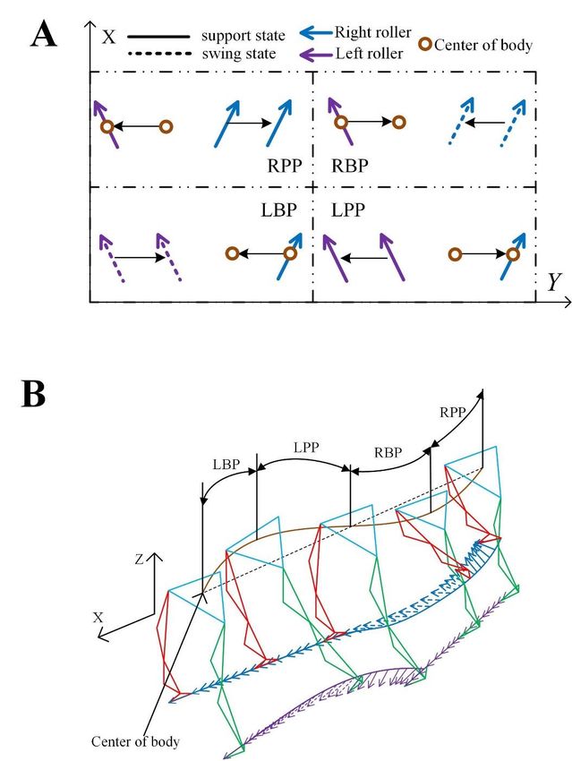
The demarcation between RPP and RBP is the moment that the toe marker of right skate leaves from the ground.
The body and left leg can be regard as a rigid body without relative motion. The swing height of right leg is as small
as possible without the ground reaction force (GRF) for decreasing energy consumption generated by wiggle. The
center of body slide along the direction of left passive wheels with stability.
Left Push Phase (LPP):
The demarcation between RBP and LPP is the moment that heel of right skate falls to the ground. The center of body
moves from left leg to right leg with a thrust is generated by left leg. The left roller skate has no relative motion with
ground when the thrust between the right skate and ground is generated. Most vertical supporting force of body is
provided by right leg. The heel of left skate leaves from the ground before the center of body closes to the line of
support skate.
Left Back Phase (LBP):
The demarcation between LPP and LBP is the moment that the toe marker of left leg leaves from the ground. The
body and right leg can be regard as a rigid body without relative motion. The swing height of left leg is as small as
possible without GRF for decreasing energy consumption generated by wiggle. The center of body slides along the
direction of right passive wheels with stability. The demarcation between LBP and RPP is the moment that the heel
of left skate falls to the ground.
 According to the data of experiment results from all participants, the time of RPP, RBP, LPP and LBP are about
10%~15%, 35%~40%, 10%~15% and 35%~40% of the whole cycle, respectively. The direction of the right and left
passive wheels are shown as Fig. 2 (A) in one cycle of the linear gait for all participants. In Fig. 2 (A), the angle
between the X axis of body and the passive wheel of the supporting skate remains about 10-20°. The direction of the
passive wheels of the supporting skate in LBP and RBP for five participants shown as Tab. 1 is the individual
difference in the linear gait. The angle of left and right skates has a certain differences with a small range. In RBP
and LBP, the body is controlled to be consistent with the supporting leg for a stable movement. The angle between
the X axis of body and the passive wheel of swing leg without obvious features is dependent on the line motion for
the body balance.
 The position of roller skates and center of body can be expressed as an ‘S’ curve in 3D space as shown in Fig.
2 (B) and (C). In RBP and LBP, the value of the center of body along Y axis becomes bigger then smaller while the
height of center of body becomes higher then lower. In the horizontal plane, roller skate motion is an apparent linear
move along the direction of supporting passive wheels in RBP and LBP. The skate height of swing leg is about 50
mm for reducing energy consumption.
 The relative position from the center of body to left roller skate in RBP and the relative position from the center
of body to right roller skate in LBP in the skating coordinate system are shown in Fig 2 (D) and (E). The relative
position from the center of body to the supporting leg shows the same feature in the skating coordinate systems. In
the skating coordinate system, the value of X axis and Y axis has a large fluctuation. The value of Z axis shows a
small fluctuation, first rise and then fall, and remains about 800 mm.
The characteristics of the turning gait
According to the turning gait experiments of human roller skating, one gait cycle of the turning gait can be divided
into 3 phases (Fig. S2).
Enter Turning State (ETS):
After the speed of supporting passive wheels is enough quick, the center of body transfers to left and the sagittal
plane rotate to be parallel to the skating plane of left leg by the hip rotation. The roll angle between the passive wheel
of left skate and the Z axis of body increases for gaining a spin angular velocity of body. The supporting force
provided by left leg is gradually increasing.
 Biology Open • Accepted manuscript

Remain Turning State (RTS):
This phase can be skipped while the expected spin angle of body is small. When the roll angle between the passive
wheel of left skate and the Z axis of body remains a specific value, the body enters a state of equilibrium without
any joint movement in the absence of friction loss. Most supporting force is provided by left leg and right leg is
utilized to keep balance. The angle between the right passive wheel and body remains about 15° in order to control
the turning radius while the right foothold is behind the center of body along the X b axis. The friction and initial
speed determine the time that the invariable posture of the whole body can be maintained.
Quit Turning State (QTS):
When the aim direction of the turning gait is almost realized, the center of body can return to the middle of two legs.
QTS can be regarded as the inverse process of ETS.

 Downloaded from http://bio.biologists.org/ by guest on January 8, 2021

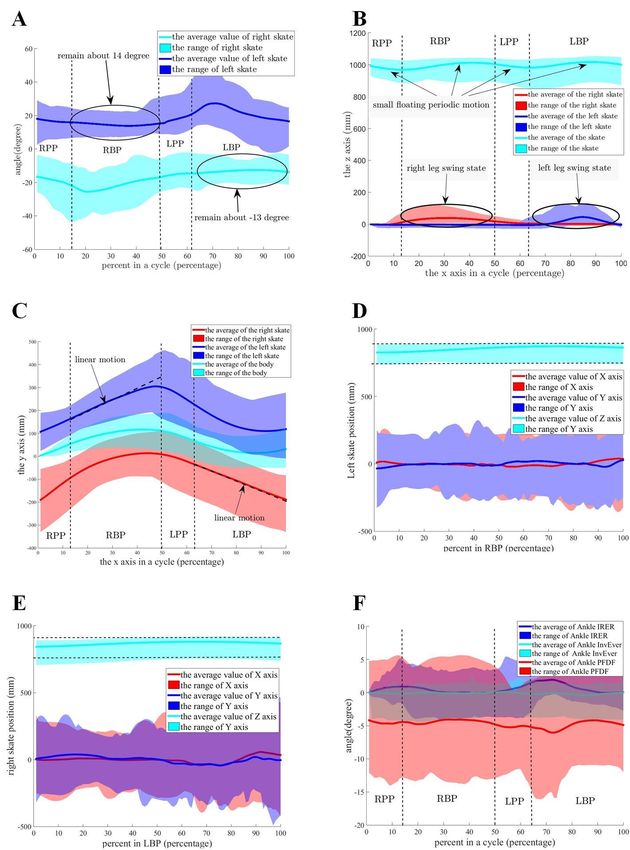
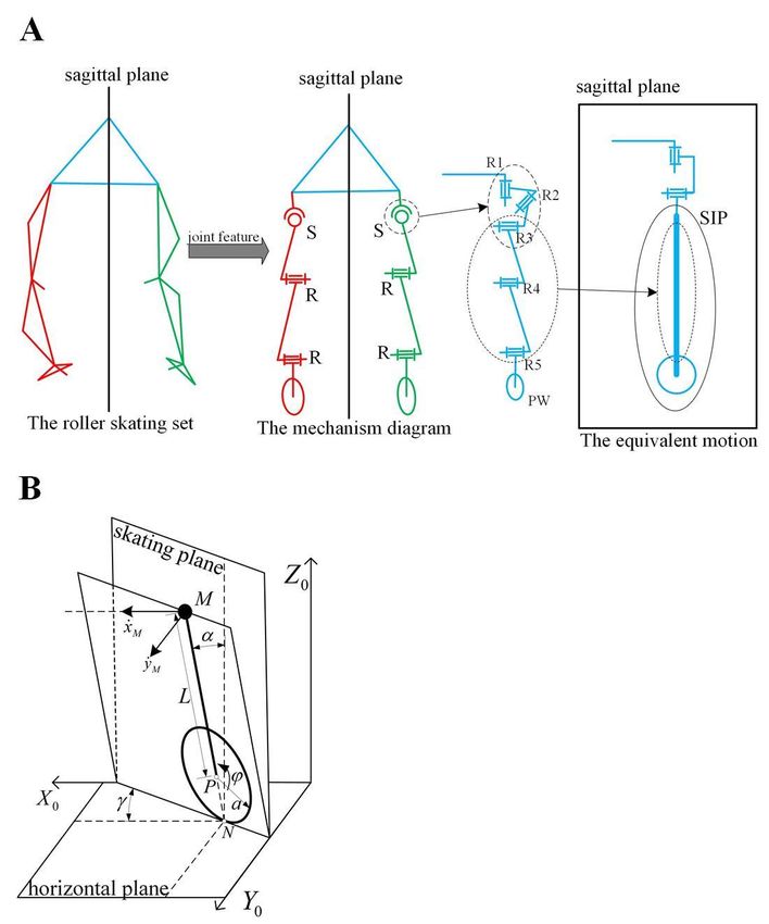
The roll angles of passive wheels in the turning gait are shown in Fig. 3 (A). The roll angle of left skate increases
when participants enter RTS and returns the initial value when participants quit RTS. The roller angle of left skate
has a small change in RTS for a short time. The passive wheel of right skate with tremendous float plays an important
role of auxiliary balance and controlling the turning radius of body. Because there is no relative motion between the
center of body and left skate in RTS, the spin angular speed of left skate can be regarded as the spin angular speed
of body.
 The spin angular velocity and turning radius of passive wheel for all participants are expressed in Fig. 3 (B)
and (C). In Fig. 3 (B), the spin angular velocity of left skate remains about 55 °/s and the turning radius of left skate
is about 2.3 m with a small floating in RTS. But the turning radius of body has a great disturbance when the
participant enters and quits the turning gait. A signally chaos shown in the spin angular speed and turning radius of
right skate reveals the constraint between right skate and ground is a special non-holonomic constraint with sliding
friction. The angle between the X axis of body and the passive wheel direction of right skate is used to remain the
turning radius of body using the feature of non-holonomic constraint. The kinematics characteristics of right skate
indicate the primary function of right skate is to control the spin angular velocity of body utilizing the lateral force
of passive wheel. The primary function is also confirmed by the phenomenon the angle between the left and right
skate passive wheel remains a constant value. The relative position between left and right skate foothold is another
factor to control the turning radius of body. The turning radius and roll angle of body are decided by the passive
wheel speed of left skate when the participant enters the turning gait. The turning gait is different to be achieved
when the initial speed of passive wheel is too slow or too fast. The average spin angular velocity and turning radius
of passive wheels in RTS for all participants is shown in Tab. 2. In order to achieve the same radius of circular
movement, the spin angular velocity remain similar to each other.
 The relative position from the center of body to left skate of RTS in the skating coordinate system is shown in
Fig 3 (D). The relative position from the center of body to left skate of RTS remain unchanged for the stable turning
radius. The value of Z S axis shows a small fluctuation and remains about 0.8 m. A small change shows the expected
motion of body while the participant wants to control the stability on the movement direction of passive wheel along
the X S axis.

DISCUSSION
The joint feature of the roller skating gait
The motion characteristics of roller skating are decided by the bone structure of human. The analysis of human
structure based on the new roller skating model benefits understanding the internal cause of the motion
characteristics of roller skating. The roller skating model for expressing the motion of human roller skating is similar
to the typical Helen Hayes model for describing the motion of human walking. Seven segments in the roller skating
model consist of one pelvis, two thighs, two shank and two roller skates. Three main joints whose movement is
expressed in Fig. 1 (D) are defined as hip joint, knee joint and ankle joint, similar to the Helen Hayes model. The
hip joint of the roller skating set connects a pelvis and a thigh. The knee joint connects a thigh and a shank. The
ankle joint connects a shank and a roller skate.
 The hip joint can be regarded as a spherical joint with three DOFs. The ankle and knee in the roller skating
model are modified based on the feature of roller skating. In traditional Helen Hays model, the ankle joint can be
regarded as a spherical joint with three DOFs. Three DOFs of the ankle joint are named as Ankle_PFDF,
Ankle_InvEver and Ankle_IRER. Their variations in the linear and turning gait are shown in Fig. 2 (F) and Fig. 3
(E). In the linear gait, the Ankle_PFDF angle of supporting leg remain a constant with a large range for all passive
 Biology Open • Accepted manuscript

wheels touching the ground. The angle of Ankle_InvEver and Ankle_IRER remain about 0 degree with a small
fluctuation when the leg is a supporting state. In the turning gait, the Ankle_PFDF angle of supporting leg has a
change following the height of body with a large range for stability. The angle of Ankle_InvEver and Ankle_IRER
show small fluctuation. According to the features of the angle joint for roller skating, the ankle joint can be regarded
as a revolute named as Ankle_PFDF. In the roller skating model, Ankle_InvEver and Ankle_IRER of ankle without
impacting the motion characteristics can be ignored. In traditional Helen Hays model, the ankle joint can be regarded
as a spherical joint with one DOFs named as Knee_FE.
The derivation of one supporting leg
 One supporting leg model of human roller skating described as a simply wheel model is difficult to fit the
experiment results. Base on the characteristics of body motion and all joints, a new model named as the skating
inverted pendulum (SIP) for one supporting leg is built to simplify the roller skating feature. The derivation from
the real roller skating to the SIP model can be expressed in Fig. 4 (A). The hip, knee and ankle joints of the roller
skating set can be regarded as a spherical, a revolute and a revolute joint based on the feature of all joints respectively.

 Downloaded from http://bio.biologists.org/ by guest on January 8, 2021

The passive wheel constraint (PW) of supporting leg consists of one revolute and one typical non-holonomic
constraint. The mechanism diagram of one supporting leg can be expressed as an S-R-R-PW serial mechanism from
the traditional Helen Hays model in Fig. 4 (A). The axis of passive wheel is perpendicular to the sagittal plane in the
initial state. The axis of this two revolute joints is parallel to each other and is parallel the axis of passive wheel in
the initial state. Based on the theory of mechanism, one spherical joint can be decomposed as three revolute joints
named as R1, R2 and R3. The axis of R1 is parallel to the gravity. The axis of R2 is parallel to the direction of passive
wheel in the sagittal plane. The axis of R3 is parallel to R4. The combination of R3, R4 and R5 can be equivalent to
an inverted pendulum that is perpendicular to the direction of passive wheel in the sagittal. In the linear gait, R1 is
utilized to adapt the angle between the sagittal plane and the direction of passive wheel. Part of the spin force to
achieve the turning gait is generated by R1. R2 is used to generate the roller angle for the SIP model and the torque
to keep the body balance. SIP including R3, R4, R5 and PW is used to describe the motion characteristics of human
roller skating. SIP different from the traditional plane locomotion on the vertical plane is three dimensional motion
because the contact between the passive wheel and ground is a non-holonomic constraint. The motion feature of SIP
decides the characteristics of roller skating based on one supporting leg. When values of R1 and R2 are not equal to
zero, the sagittal plane should change to the skating plane for showing the motion characteristics of the SIP model.

The characteristics of SIP model
The SIP model consisted of an equivalent rigid body, an equivalent link and a virtual passive wheel can be expressed
as Fig. 4 (B).
 In Fig. 4 (B) M, P and N are points of the center of body, the center of the virtual passive wheel and the contact
between the passive wheel and ground respectively. The mass and moment of inertia of the equivalent body are mM
 J J z  . The equivalent link whose mass and moment is ignored has a rigid connection with the rigid
 T
and x Jy
body. The virtual passive wheel whose mass and moment is ignored has a revolution joint with the equivalent link
whose length is . The radius and angle of passive wheel are a and . The orientation of the rigid body can be
described that rotating  about the Z axis after rotating  about the X axis. Based on the feature of non-
holonomic constraint, the kinematics of the rigid body can be expressed as (proposed in appendix 1 in detail)
  xM   L  a   sin  cos     cos  sin     a cos 
 
  yM   L  a    cos  cos     sin  sin     a sin  (6)
  z = L+a cos 
  M  
where xM , yM is the velocity of body along X 0 , Y0 axis and zM is the height of body.
 According to the Lagrange equation, the dynamic of the rigid body about  ,  , can be expressed as (proposed
in appendix 1 in detail)
     A1    sin  cos   A2   cos   A3 sin  +B1 
 2

 
   A6 sin      A7    cos + B2 sin 2  +B3 cos 2  c      sin 
      
  A4 sin 2   A5 cos 2  A4 sin 2   A5 cos 2  (7)
 
    8   9     10     B sin   B5 cos 
 2
 A sin A A sin 2 2

     cos  + 4 2 c      sin   sin 
  A4 sin 2   A5 cos 2  A4 sin   A5 cos 2 

where Ai  i  1,,10 , Bi  i  1,,5 is constant about mM ,  J x J z  ,   is the moment for the
 T
 Jy
balance of the rigid body, c is the damping torque coefficient of the Z axis generated from frictional resistance.
 Biology Open • Accepted manuscript
 The dynamic model of SIP with an integral about the time is different to be described. We pay attention to the
special stable state of SIP, the linear motion and circular motion.
The linear motion:
 The boundary condition of the linear motion can be expressed as  =0 ,  =0 ,  =0 ,  = 0 ,  =0 ,  =0
satisfied the dynamic equation of SIP.  0 is a constant and 0 is a constant that is not zero. The motion of the
rigid body can achieve the linear motion described as
  xM  0 a cos  0
 
  yM  0 a sin  0 (8)
  z =L +a
  M
 The special boundary condition of the linear motion is utilized to keep the linear gait of human roller skating
with one supporting leg. The supporting leg of the linear gait shows the same feature as the SIP model and moves
along the direction of passive wheels. In LBP and RBP, the center of body is controlled on the line of supporting
passive wheels. The axis of supporting passive wheels remain to be parallel to the horizontal plane.

 Downloaded from http://bio.biologists.org/ by guest on January 8, 2021

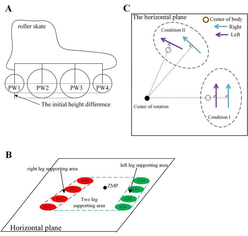
The circular motion:
 The boundary condition of the circular motion is similar to the linear motion with a different initial value    0 .
The boundary condition of the circular motion can be expressed as  =0 ,  =0 ,  =0 ,  = 0 ,  =0 .  0 and 0
that is not zero is satisfied the condition that    0 . The motion of the rigid body can achieve the circular motion
described as
  xM   L  a   0 sin  0  0 a  cos  0t
 
 
  yM   L  a   0 sin  0  0 a  sin  0t (9)
 
  zM =  L +a  cos  0
 
 In the special circular motion, the trajectory of the rigid body is a circle in the horizontal plane. The turning
radius of the center of body in the boundary condition of the circular motion is
 
 RB   L  a  sin  0  a 0 (10)
  0
 The turning radius of the circular motion is decided by  0 and 0 that is a free DOF without directly
controlling. According to the dynamic of SIP from the linear motion to the circular motion, the spin velocity
generated by a roll velocity can be used to turn instead of the direct control from the spin force. The spin angular
velocity (   ) of center of body can be generated by hip joint with a huge moment. For improving the energy
utilization in the turning gait, the special dynamic characteristic of SIP is used to generate the spin angular velocity.
The spin angular speed adjusted by the roller angle from zero to  0 controls the turning radius with the passive
wheel speed ( 0 ).

Strategy of the roller skating
In this section, the method using SIP to enhance the stability in the linear gait and the efficiency in the turning gait
is discussed.
 In order to analyze the stability of human roller skating, the zero moment point (ZMP) (Vukobratovic, M., &
Borovac, B.)(Potkonjak, V.) used for analysis of the human and robot motion stability is selected to be the stability
criterion. Different from the traditional human walking, the contact area of the human roller skating between one
passive wheel and the ground is very small. So the structure with one passive wheel is different to keep stability. In
real roller skate, four passive wheels named as PW1, PW2, PW3 and PW4 are collinear in Fig. 5 (A). The radius of
PW2 and PW3 is great than PW1 and PW4. The contact area between one roller skate and the ground including four
disconnected small area increase the supporting area. The supporting area of human roller skating based on ZMP is
shown as Fig. 5 (B). The contact area of the left skate PW1, PW2, PW3 and PW4 are LN1, LN2, LN3 and LN4. The
contact area of the right leg PW1, PW2, PW3 and PW4 are RN1, RN2, RN3 and RN4. The supporting area of human
roller skating with two supporting skates utilizing the structure of roller skate is close to the area of walking. The
human roller skating with two supporting skates has better stability, such as RPP and LPP. The supporting area with
one supporting is close to a line, such as RBP and LBP. The stability of human roller skating with one supporting is
different to controlled on the axis of passive wheels. The movement of the supporting skate is important to control
the ZMP for the stability. The movement of R3, R4 and R5 equivalent to the planar motion can adapt the equivalent
inverted pendulum to be perpendicular to the direction of passive wheel in the skating plane. The equivalent inverted
pendulum is difficult to be perpendicular to the direction of passive wheel while the supporting skate has one passive
wheel. The stable area is proportional to the distance between centers of PW1 and PW4. The stability of roller skating
can be improved by the structure of roller skate. So the mass dumping along the direction of passive wheel is not
 Biology Open • Accepted manuscript
considered in the SIP model. In the linear gait, the passive wheel of supporting skate is controlled to be perpendicular
to the horizontal plane in order to the linear motion based on SIP. The center of body is controlled between centers
of PW1 and PW4 for stability roller skating.

 Downloaded from http://bio.biologists.org/ by guest on January 8, 2021

Based on SIP, the rotating motion of roller skating can be generated by rolling passive wheels. However, the
frictional resistance generated by the structure of four passive wheels is too large to difficult to achieve the turning
gait with a small radius. The difference between four passive wheels and the cooperative work of two legs play a
significant part of the turning gait with a small radius. The initial height difference can be utilized to decrease the
frictional resistance while the touch point between the four passive wheels and ground is not collinear. The touch
point between the four passive wheels and ground can be regarded as the point of circle arc in RTS for improving
the effect of rotation. In RTS of the turning gait, the direction and position of passive wheels can be divided into two
condition shown in Fig. 5 (C). In the condition I, the passive wheel axis of two legs is collinear. The turning gait
with a small radius is difficult to be obtain while the whole of body can be regarded as a holonomic constraint of a
rectilinear motion in the condition I. Because the whole of body can be regarded as a holonomic constraint of a
rotary motion in the condition II, the condition II is selected to achieve the turning gait with a small radius by the
participants in the process of experiment.

CONCLUSION
 Based on the motion characteristics of the roller skating, the linear gait can be divided into four phases and the
turning gait can be divided into three phases. The spin angle between the sagittal plane and the roller skate of
supporting leg is mainly generated by the external/internal rotation of hip joint instead of ankle. In RBP and LBP of
the linear gait, the motion of the body and supporting skate along the direction of supporting passive wheels shows
the same feature. In the turning gait, the spin angular of body with one supporting leg mainly is generated by the
roller angle of passive wheels. The SIP model is built to describe the center of body with one supporting leg in the
linear gait and turning gait. Utilizing the structure of the roller skate with four passive wheels to improve the stability,
the SIP model ignores the DOF of rotating the Y axis in the body coordinate system. The method to achieve a turning
gait with a small radius is to use two non-holonomic constraints of two legs. The motion characteristics of human
roller skating shows the same feature with the SIP model on the special state. In the feature work, the roller skating
robot can use the SIP model and this method to improve the stability and efficiency.

Acknowledgement
This work was supported by the National Natural Science Foundation of China (Grant No. 51775011).

APPENDIX I
The kinematics and dynamic of the SIP model is derived in detail.
According to the hypothesis in this paper, the orientation of the rigid body is
 cos   cos  sin  sin  sin  
 R M   sin  cos  cos   sin  cos   .
  0 sin  cos  
The unit vector of the passive wheels axis is
 yW    cos sin  cos cos  sin   .
 T

The unit vector of the equivalent inverted pendulum axis is
 zW = sin  sin   cos  sin  cos 
 T

The angular velocity of the rigid body is
 w M =   cos    sin   
 Biology Open • Accepted manuscript
 T

Without the slipping between the passive and the ground, the velocity of N point that is zero can be expressed as
 v N  v M  w M   L  a   zW  + yW   a  zW   0 (I.1)

Eq. (I.1) can be simplified as Eq. (6).
 xM   L  a   sin  cos     cos  sin     a cos 

 yM   L  a    cos  cos     sin  sin     a sin 
 z = L+a cos 
 M  
Suppose that the generalizing DOF is defined as q   xM    .
 T
 yM zM
The non-holonomic constraint of the SIP can be defined as
  1 =xM   L  a   sin  cos     cos  sin     a cos 
 
  2  yM   L  a    cos  cos     sin  sin     a sin 
  =z  L +a cos 
  3 M  

 Downloaded from http://bio.biologists.org/ by guest on January 8, 2021

The whole energy of system is
 T
 1
 2
  mM v2M +wTM JW w M  +mM gzM .
The damp of the ground is c     sin  0 0 1 .
 T

The driving force is   cos  sin  0 .
 T

According to the Lagrange equation, the dynamic of SIP is
 d T T   
   Qi  Pi +1 1 +2 2 +3 3
 dt qi qi qi qi qi (I.2)
  i  0,1,2,3,4,5,6 
Where 1, 2 , 3 are undetermined multipliers
Eq. (I.2) can be simplified as Eq. (7) without i .
    A1    sin  cos   A2   cos   A3 sin  +B1 
 2


  A6 sin      A7    cos + B2 sin 2  +B3 cos 2  c      sin 
     
 A4 sin 2   A5 cos 2  A4 sin 2   A5 cos 2 

   A8 sin   A9      A10 sin     B sin 2   B5 cos 2 
 2

   cos  + 4 2 c      sin   sin 
 A4 sin   A5 cos 
 2 2
 A4 sin   A5 cos 2 
 J y  J z +mM  L  a 
 2
 J y +mM a  L  a  mM g  L  a 
 A4  J y mM L2 , A5  J z  J y  mM a 2 
 1
A1 = ，A2 = A3 = ，B1 =
 J x +mM  L  a  J x +mM  L  a  J x +mM  L  a  J x +mM  L  a 
 2 2 2 2

A6   J y  mM a 2  mM La  2mM L2  J y   2 A5 A7   J y  J y  mM a 2  , B2  mM La, B3    J y  mM a 2 

 J  mM aL  mM a 2   J y mM L2  A5
 2

A8  J y
 y
 A9   J z  J y  2mM aL  2mM a 2  , A10  J y  J y  mM aL  mM a 2 
 J y  mM a 2
B4  mM L  L  a  , B5  J y  mM a  L  a   J z

 Biology Open • Accepted manuscript

 Downloaded from http://bio.biologists.org/ by guest on January 8, 2021

REFERENCES
Baker, R. (2006). Gait analysis methods in rehabilitation. Journal of NeuroEngineering and Rehabilitation, 3(1), 4.
Mcginley, J. L., Baker, R., Wolfe, R., & Morris, M. E. (2009). The reliability of three-dimensional kinematic gait measurements:
a systematic review. Gait & Posture, 29(3), 360-369.
Nagahara, R., Matsubayashi, T., Matsuo, A., & Zushi, K. (2014). Kinematics of transition during human accelerated
sprinting. Biol Open,3(8), 689-699.
Vaughan, C. L., Davis, B. L., & O'Connor, J. C. (1999). Dynamics of human gait. Human Kinetics Publishers.
Kadaba, M. P., Ramakrishnan, H. K., & Wootten, M. E. (1990). Measurement of lower extremity kinematics during level
walking. Journal of Orthopaedic Research Official Publication of the Orthopaedic Research Society, 8(3), 383-92.
Żuk, Magdalena, & Pezowicz, C. A., (2015). Kinematic analysis of a six-degrees-of-freedom model based on isb
recommendation: a repeatability analysis and comparison with conventional gait model. Applied Bionics and
Biomechanics,2015,(2015-1-29), 2015, 1-9.
Lay, A. N., Hass, C. J., & Gregor, R. J. (2006). The effects of sloped surfaces on locomotion: a kinematic and kinetic analysis.
Journal of Biomechanics, 39(9), 1621-1628.
Yosibash, Z., Wille, H., & Rank, E. (2015). Stochastic description of the peak hip contact force during walking free and going
upstairs. Journal of Biomechanics, 48(6), 1015-22.
Schache, A. G., Baker, R., & Vaughan, C. L. (2007). Differences in lower limb transverse plane joint moments during gait when
expressed in two alternative reference frames. Journal of Biomechanics, 40(1), 9-19.
Brown, H. B. (1986). Running on four legs as though they were one. IEEE Journal of Robotics & Automation.
Ramirez, R. (1983). Dynamics of non-holonomic systems. , 6.
DING Xilun, ZHENG Yi, & XU Kun. (2017). Wheel-legged hexapod robots:a multifunctional mobile manipulating platform.
Chinese Journal of Mechanical Engineering, 30(1), 3-6.
Kooijman, J. D., Meijaard, J. P., Papadopoulos, J. M., Ruina, A., & Schwab, A. L. (2011). A bicycle can be self-stable without
gyroscopic or caster effects. Science, 332(6027), 339-42.
Iverach-Brereton, C., Baltes, J., Anderson, J., Winton, A., & Carrier, D. (2014). Gait design for an ice skating humanoid robot.
Robotics & Autonomous Systems, 62(3), 306-318.
GenEndo, & ShigeoHirose. (2012). Study on roller-walker — improvement of locomotive efficiency of quadruped robots by
passive wheels. Advanced Robotics, 26(8-9), 969-988.
Stefanucci, J. K., Proffitt, D. R., Clore, G. L., & Parekh, N. (2008). Skating down a steeper slope: fear influences the perception
of geographical slant. Perception, 37(2), 321-323.
Hettinga, F. J., Koning, J. J. D., Schmidt, L. J. I., Wind, N. A. C., Macintosh, B. R., & Foster, C. (2011). Optimal pacing
strategy: from theoretical modelling to reality in 1500-m speed skating. Br J Sports Med, 45(1), 30-5.
de Koning, J. J., Foster, C., Lampen, J., Hettinga, F., & Bobbert, M. F. (2005). Experimental evaluation of the power balance
model of speed skating. Journal of Applied Physiology, 98(1), 227-233.
Nobes, K. J., Montgomery, D. L., Pearsall, D. J., Turcotte, R. A., Lefebvre, R., & Whittom, F. (2003). A comparison of skating
economy on-ice and on the skating treadmill. Can J Appl Physiol, 28(1), 1-11.
Vukobratovic, M., & Borovac, B. (2004). Zero-moment point: thirty years of its life. International Journal of Humanoid Robotics,
1, 157-173.
Potkonjak, V. (2012). Human-and-humanoid motion - distinguish between safe and risky mode. IFAC Proceedings Volumes,
45(22), 524-529.

 Biology Open • Accepted manuscript

 Downloaded from http://bio.biologists.org/ by guest on January 8, 2021

Tab. 1 the average angle between the X axis and passive wheels for five participants
 Participant
 Left skate in RBP(°) Right skate in LBP(°)
 number
 1 16.3 -11.7
 2 14.5 -12.3
 3 14.6 -11.6
 4 11.8 -15.5
 5 12.7 -17.1
 all 14.4 -13.3
Tab. 2 the average spin angular velocity and turning radius in RTS for five participants
 Participant
 spin angular velocity(°/s) turning radius(m)
 number
 1 49.9 2.30
 2 63.3 2.11
 3 56.6 2.26
 4 52.6 2.43
 5 49.1 2.46
 all 54.1 2.32

 Biology Open • Accepted manuscript

 Downloaded from http://bio.biologists.org/ by guest on January 8, 2021

Figures

 Biology Open • Accepted manuscript

Fig. 1 The roller skating model (A) the marker set (B) the skating plane (C) the critical parameter(D)the joint set

 Downloaded from http://bio.biologists.org/ by guest on January 8, 2021

Biology Open • Accepted manuscript

Fig. 2 The characteristics of the linear gait for human roller skating for all participants (A) the angle between the X
axis of body and passive wheels in cycle (B) the Z-X position of roll skates and the center of body in the ground
coordinate system (C) the Y-X position of roll skates and the center of body in the ground coordinate system (D)
the relative position from the center of body to the left skate in the skating coordinate system in RBP (E) the
relative position from the center of body to the right skate in the skating coordinate system in LBP (F) the angle of
ankle joint

 Downloaded from http://bio.biologists.org/ by guest on January 8, 2021

Biology Open • Accepted manuscript

Fig. 3 The characteristics of the turning gait for human roller skating (A) the roll angle of passive wheels in the
turning gait for all participants (B) the spin angular velocity of the turning gait in a cycle for all participants (C) the
turning radius of the turning gait in a cycle for all participants (D) the relative positon from the center of body to
left skate of RTS in the skating coordinate system (E) the angle of ankle joint

 Downloaded from http://bio.biologists.org/ by guest on January 8, 2021

Fig. 4 The derivation and model of SIP (A) the derivation from the real roller skating to SIP (B) the model of SIP

 Biology Open • Accepted manuscript

 Downloaded from http://bio.biologists.org/ by guest on January 8, 2021

Fig. 5 The real structure of human roller skating (A) the real structure of roller skate (B) the supporting area of
human roller skating (C) the condition of cooperative work in RTSss

 Biology Open • Accepted manuscript

 Downloaded from http://bio.biologists.org/ by guest on January 8, 2021

Biology Open (2019): doi:10.1242/bio.037713: Supplementary information

 Fig. S1 The linear gait of human roller skating (A) the vertical view in body coordinate system (B) the Biology Open • Supplementary information
 obligue view in the ground coordinate system

 Downloaded from http://bio.biologists.org/ by guest on January 8, 2021

Biology Open (2019): doi:10.1242/bio.037713: Supplementary information

 Biology Open • Supplementary information
 Fig. S2 The turning gait of human roller skating (A) the vertical view in body coordinate system (B) the
 obligue view in the ground coordinate system

 Downloaded from http://bio.biologists.org/ by guest on January 8, 2021

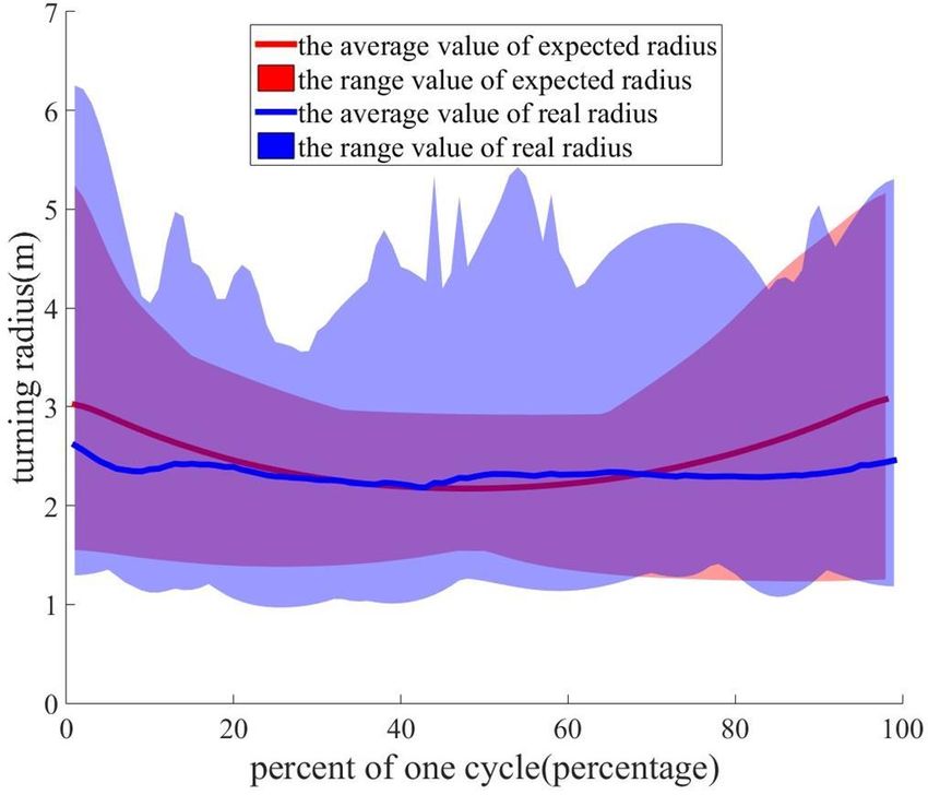
Biology Open (2019): doi:10.1242/bio.037713: Supplementary information

 Fig. S3 The real and expected radius of body in the turning gait for all participants. The real radius of body is
 computed by the curvature in the ground coordinate system. The expected radius of body is calculated by the SIP
 model. The real radius remains about 2.5m and the expected radius changes between 3m and 2.5m.

 Biology Open • Supplementary information

 Downloaded from http://bio.biologists.org/ by guest on January 8, 2021

Biology Open (2019): doi:10.1242/bio.037713: Supplementary information

 Fig. S1 The linear gait of human roller skating (A) the vertical view in body coordinate system (B) the Biology Open • Supplementary information
 obligue view in the ground coordinate system

Biology Open (2019): doi:10.1242/bio.037713: Supplementary information

 Biology Open • Supplementary information
 Fig. S2 The turning gait of human roller skating (A) the vertical view in body coordinate system (B) the
 obligue view in the ground coordinate system

Biology Open (2019): doi:10.1242/bio.037713: Supplementary information

 Fig. S3 The real and expected radius of body in the turning gait for all participants. The real radius of body is
 computed by the curvature in the ground coordinate system. The expected radius of body is calculated by the SIP
 model. The real radius remains about 2.5m and the expected radius changes between 3m and 2.5m.

 Biology Open • Supplementary information