Multi-lens, Multi-camera Calibration of Sony Alpha NEX 5
←
→
Page content transcription
If your browser does not render page correctly, please read the page content below
Multi-lens, Multi-camera Calibration of Sony Alpha NEX 5
                                     Digital Cameras
                                                    M. R. Shortis
                                  School of Mathematical and Geospatial Sciences
                              RMIT University, GPO Box 2476 Melbourne 3001, Australia
                                              mark.shortis@rmit.edu.au

Abstract
This paper describes close-range calibrations of multiple Sony Alpha NEX 5 consumer digital cameras with multiple
interchangeable lenses.     The standard physical parameter set and a standard parameter set with affinity and
orthogonality terms are tested with both block-invariant and photo-invariant principal point parameters. The impact of
the parameter sets is analysed to determine the effectiveness of the inclusion of these parameters in reducing
systematic errors. The parameters are analysed to determine if a lens effect or camera effect is being modelled. Some
conclusions are drawn regarding the possible physical sources of the systematic errors.
Key words: photogrammetry, close-range, calibration, parameters, multi-camera, multi-lens, stability
Author Biography

Mark Shortis is Professor of Measurement Science in the School of Mathematical and Geospatial Sciences and Director, Program
Quality in the College of Science, Engineering and Health at RMIT University in Melbourne, Australia. Since the early 1980s he
has been active in research in photogrammetry at close range, for example collaborative research with NASA Langley Research
Center on the structural dynamics of aerospace models, with the University of Western Australia on underwater assessment of
marine fish populations and habitats, with DLR Germany on the characterisation of solar concentrators for energy generation and
with CSIRO Marine Research on deep water seabed mapping.

Introduction

To determine accurate measurements using close range photogrammetry, cameras must be calibrated. The parameters
and techniques used for the calibration of cameras at close range are well established (Brown, 1971; Fryer, 1996,
Fraser, 1997; Remondino and Fraser, 2006). Self-calibration using a calibration fixture or the measurement object is
the accepted technique for the modelling and elimination of the systematic errors which would otherwise adversely
affect the accuracy of the photogrammetric measurements (Kenefick et al., 1972). The details of the photogrammetric
network solution based on collinearity and an iterative, least squares estimation solution are described in Granshaw
(1980). In order to confidently derive the calibration parameters, the geometry of the photogrammetric network
should be multiple, convergent photographs of a three dimensional target array or calibration fixture, preferably with a
range of camera to object distances and a variety of orthogonal roll (rotation about the camera axis) angles to reduce
correlations between parameters (Kenefick et al., 1972).
Previous camera calibrations, particularly in the field of high accuracy metrology, have demonstrated that camera
calibration parameters can compensate for distortion effects that have no readily associated physical meaning. A
typical example is the continued use and statistical significance of the image affinity term with the standard physical
parameter model for camera calibration of both close-range (Reulke, 2006) and aerial (Cramer, 2004) digital cameras.
This parameter was designed to compensate for affine film shrinkage, yet the parameter is still used regularly in
calibration models for cameras with digital image sensors. An orthogonality term is also used in parameter sets to
account for non-orthogonality of the x-y image coordinates, also known as image shear. Orthogonality is perhaps less
frequently used and is only rarely reported as a significant term in the calibration set. Nevertheless, even though the
physical effect of image
shear is associated with photographic film, not with CCD and CMOS image sensors, the term is included in the ’10
parameter’ calibration set (Fraser, 1997). Both parameters are included in many close-range photogrammetry network
adjustment software applications, for example Australis 1 and AICON 3D Studio 2.
1
    www.photometrix.com.au
2
    www.aicon.de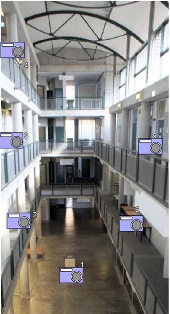
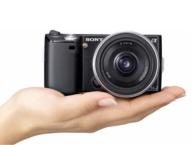
Calibration Parameters

Camera calibration at close-range is most often based on a set of physical parameters comprising the principal distance
(PD), principal point (PP) location, radial and decentring lens distortions (Fraser, 1997). The primary physical
parameters of the calibration define the location of the lens perspective centre with respect to the image sensor and the
lens distortions that represent the departures from a perfect central projection. Radial and decentring lens distortion
characteristics have been well established through extensive testing and validation over several decades since the
initial formulation of the models (Brown, 1966; Ziemann and El-Hakim, 1983). One recent review has suggested that
this physical parameter set is sufficient and extra parameters are not necessary for digital cameras (Remondino and
Fraser, 2006). This contention is supported by calibrations that include these parameters but the analysis indicates that
affinity and orthogonality are not significant (Chikatsu and Takahashi, 2009; Wendt and Dold, 2005), even when used
with large area image sensor arrays (Mills et al., 2003; Rieke-Zapp, 2010).
A review of physical, empirical and combinations of types of additional parameters to model the secondary image
non-linearities and image plane unflatness is given in Faig and Shih (1988). However because of the geometric
regularity and stability of the sensor combined with digital transmission of the pixel data (Shortis and Beyer, 1996),
modern CCD and CMOS sensors should not be subject to the classic image deformations associated with film or glass
plate cameras (Fraser, 1997). Nevertheless both Fraser et al. (1995) and Shortis et al. (1995) found that the affinity
term in the camera calibration parameter set was highly significant. Fraser et al. (1995) reports that the affinity term is
strongly correlated with lenses, rather than cameras, in a calibration test that compared three different focal length
lenses interchanged between two different resolution digital cameras. This suggests that the affine change in scale is
associated with an optical effect rather than an image deformation. In contrast, Shortis et al. (1995) reports that the
affinity terms is strongly correlated with cameras, rather than lenses, for two different scientific CCD cameras with
two interchangeable lenses with different nominal focal lengths. This suggests that the affinity term is compensating
for a physical property of, in that case, large format area array image sensors.
One confounding factor associated with consumer quality digital cameras is the lack of stability of the camera body,
the image sensor mounting and the camera lens (Shortis et al., 1998; Rieke-Zapp et al., 2009). The poor reliability
contributes systematic errors to the camera calibration and the effects may be partially compensated by parameters
such as affinity and orthogonality.
The instability of the principal point location, caused by movement of the image sensor and the camera lens during
manual handling, can be compensated using a photo-invariant model for the principal point (Mills et al., 2003;
Moniwa, 1981; Shortis et al., 1998).         This approach associates a unique principal point location with every
photograph in the calibration network. The extra unknown terms in the least squares estimation solution tend to
weaken the network, however the impact can be lessened if the network has a strong geometry and approaches hyper-
redundancy by using many photographs and many targets (Fraser et al., 2005).

Experiment

Cameras
An opportunity arose to test the associations between calibration parameters for a ‘semi-professional’ or ‘prosumer’
compact digital camera. The opportunity was generated from the requirement to conduct a multi-camera, multi-lens
calibration of three Sony Alpha NEX 5 digital cameras (see Figure 1) acquired by the University of Queensland. The
cameras are deployed on an unmanned airborne vehicle (UAV) to capture multi-spectral imagery over mine closure
sites, in order to monitor the potential impacts of underground mining (Lechner et al., 2012; Stecha et al., 2012).
The Sony NEX 5 cameras were chosen specifically because of the ability to interchange fixed focal length lenses, as
well as the compact format, the high resolution, large area image sensor, the very light weight and relatively modest
cost. The cameras currently have available Sony 16mm ‘pancake’ lenses and in the future LEICA 35mm and 50mm
lenses will be acquired. The option of different fixed focal length lenses was a critical factor in the selection of the
camera, because of the instabilities associated with zoom lenses (Shortis et al., 2006) which would otherwise add to
the inherent instability of the body (Rieke-Zapp et al., 2009) for this class of prosumer camera.
The NEX 5 has a maximum image resolution of 4592 by 3056 pixels. The CMOS sensor is the APS-C format of 23.6
mm by 15.7 mm with a pixel spacing of 5.1 micrometres. Still images are recorded in JPEG format. The camera can
also record HDTV format video, which is useful for the aerial imagery but requires a separate calibration (Shortis,
2011).
Two of the NEX 5 cameras have an unaltered image sensor. The image sensor has the standard visible spectrum cut
filter that prevents the non-visible ultra violet and infra-red radiation reaching the CMOS array. These two cameras
are designated RGB1 and RGB2. The third camera has been altered to enable infra-red sensitivity, because the near
infra-red is important to landscape and vegetation studies. In this case the visible spectrum cut filter has been
removed so that the camera becomes a ‘full spectrum imager’, sensitive to less than 350nm in the ultra violet and up to
a wavelength of around 1000nm in the infra-red. For the mine rehabilitation application, an infra-red cut filter is
fitted to the camera lens to block frequencies of less than 720nm. This camera is designated as NIR.
After the removal of the visible light filter, the back focus of the camera must be corrected because the refraction
characteristics of the lens are altered by the change in the dominant wavelengths of light. Infra-red light is refracted
less than visible light, so the plane of best focus is displaced away from the lens. This adjustment is made using shims
or spring loaded screws, depending on the type of image sensor mounting.

                   Figure 1. Sony Alpha NEX 5 digital camera with the 16mm lens (www.sony.com)

Calibration
The three cameras must be pre-calibrated because a rigorous self-calibration is not feasible for the blocks of imagery
routinely used for the landscape monitoring. The pre-calibration information is provided as input into the aero-
triangulation software INPHO 3, used to adjust the blocks of photography captured from the UAV. The cameras must
be focussed at infinity for the pre-calibration, and it is essential that there are no unexpected correlations between
calibration parameters that may introduce systematic errors and therefore produce perturbed values for the calibration
parameters.
Accordingly, the calibration test range adopted for the pre-calibration must meet several requirements. First, the test
range must be quite versatile to accommodate the different lenses and associated fields of view. To ensure high
fidelity of the calibration parameters, especially the lens distortions, it is very important to ensure that the full format

3
    www.inpho.de
of the sensor is covered by target images. Second, a large space is required to ensure infinity focus can be used and
simultaneously retain all targets within the depth of field. Third, the test range must permit strong network geometry
to minimise parameter correlations (Kenefick et al., 1972). Finally, the test range must be permanently established to
allow for repeated calibration of the cameras to ensure the accuracy and reliability of the information derived from the
aerial imagery.
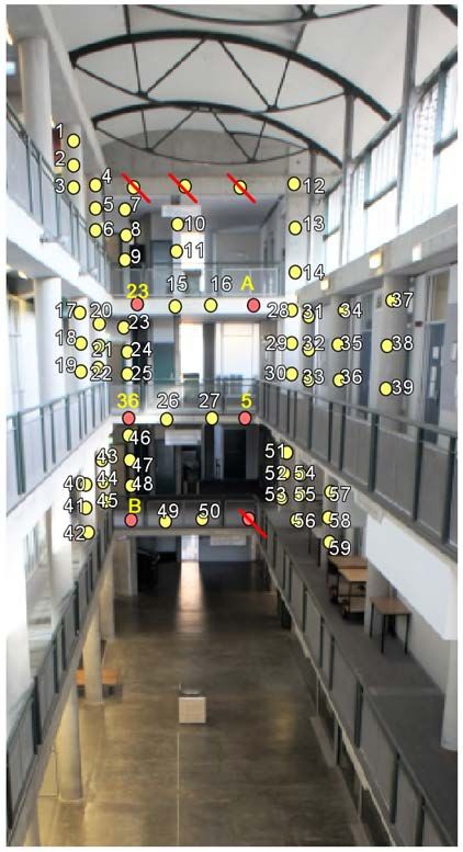
An ideal test range is provided by the atrium of one of the buildings on the University of Queensland campus (see
Figure 2). The approximate dimensions of the space are 10m by 20m by 12m, with three levels of usable volume to
place targets and four levels to position camera stations. The ground floor is deemed unsuitable for targets because of
the prominent impact on the aesthetics of the building and the potential for interference with the targets in the high
pedestrian traffic areas. The space is flexible enough for all three lens types because the long galleries allow the range
between the cameras and the targets to be varied to ensure that the target images fill the field of view of the cameras.
Approximate coordinates of the targets were determined to a precision of ±5mm using a total station.
Nine sets of calibration images were captured. Each calibration set comprised 24 exposures of the array of 62 targets
from six camera stations. The cameras were rolled into four different orthogonal orientations at each camera station.
The targets span approximately 6m by 12m by 8m in width, length and height respectively. The camera stations span
an area of 5m width by almost 10m of height. The average camera to target horizontal separation is approximately
9m.
Each of the nine camera and lens combinations were initially processed in separate self-calibrating, internally
constrained networks to determine initial calibration parameters and filter out any gross errors in the image
measurements. The network adjustments were carried out using VMS 4, which uses the standard physical model for
calibration parameters with the option of block-invariant or photo-invariant principal point parameters (Shortis et al.,
1998). The initial calibration model comprised only the primary physical parameters of block-invariant principal
point location, principal distance and lens distortions. Target coordinates were used as starting values only and were
subject to adjustment by the free network solution.
4
www.geomsoft.comFigure 2. Calibration test range: target array (left), camera stations (right). Inspection of the networks revealed that whilst some gross errors are readily attributed to problems such as partial occlusions, there is no apparent reason for a significant number of rejected image measurements near the edges of the camera format. The likely source of these rejections is the unusual radial distortion profile of the Sony 16mm lens and, in particular, the steep gradient at the edge of the field of view (see Figure 3). The gradient effectively magnifies image space errors and incorrectly classifies acceptable measurements as gross errors. In most cases these image measurements are retained in the data sets. To take advantage of hyper-redundancy (Fraser et al., 2005), the nine combinations of camera and lens were combined into one large, self-calibrating network. This network is used for the analysis of the different calibration models. The full network has more than 12000 redundancies and the average target is imaged on 106 exposures. There are just over 100 image measurements rejected by the outlier detection, with a high percentage of these near the edge of the format. Again the likely source of the concentration of rejections is the steep gradient of the radial distortion profiles. Results and Analysis A summary of the results of the self-calibrating network adjustments with the nine combinations of camera and lens is given in Table 1. Shown in the table is the RMS image residual, a prime indicator of the effectiveness of the calibration model used, and the mean precision of the target coordinates to indicate the object space precision. The table indicates clearly that a change in calibration model from block-invariant principal point to a photo-invariant principal point has a profound impact on the network, reducing the RMS image residual by half. In contrast, the inclusion of the image orthogonality and affine scale parameters has only a minor impact on the block-invariant model and no apparent improvement for the photo-invariant case.
Mean Precision of
                                                                        RMS Image
                              Calibration Model                                                  Target
                                                                       Residual (um)
                                                                                            Coordinates (mm)
             Physical parameters only, block-invariant PP                    1.24                 0.55
             Physical parameters only, photo-invariant PP                    0.63                 0.35
             Physical parameters and affinity, orthogonality,
                                                                             1.21                 0.53
             block-invariant PP
             Physical parameters and affinity, orthogonality,
                                                                             0.63                 0.35
             photo-invariant PP

Table 1. Results of the self-calibrating network adjustments with different calibration models.
Accordingly, the following results are based on the calibration model comprising physical parameters, affinity,
orthogonality and photo-invariant principal point. In all cases the values of the parameters are significant at a 95%
confidence limit.
Table 2 shows the mean principal point location in X and Y, and the principal distance for the nine combinations of
camera and lens. The principal point location is defined as the intersection of the optical axis of the lens with the focal
plane of the camera, so it would be expected that the X-Y coordinates would tend to follow the camera body. In Table
2 there is no obvious trend for the X coordinate of the principal point, which might suggest that the optical axes of the
lenses are also playing a role in the variability. The Y coordinate of the principal point has a stronger association with
the cameras than with the lenses, as indicated by the row and column standard deviations in Table 2. However there
remains a significant level of variability, confirming that the principal point location is influenced by both the position
of the sensor in the camera body and the location of the optical axis of the lens with respect to the lens mount. It is
remarkable that Fraser et al. (1995) reports a very similar outcome in that the Y coordinate of the principal point was
substantially more consistent than the X coordinate.
The unadjusted principal distances shown in Table 2 demonstrate a clear trend. The values for the two visible light
sensitive cameras, RGB1 and RGB2, indicate that the principal distance is associated with the lens, as would be
expected. The values for the NIR camera are consistently larger, by an average of 50 micrometres, reflecting the
requirement to physically adjust the back focus of this camera for the infra-red sensitivity. Mills et al. (2003) reports a
similar result for the removal of an infra-red cut filter. Once the NIR camera data is adjusted for this change, the
values of the principal distances for each lens are consistent to 1-2 micrometres.

                                                 Principal Point X (mm)
                                                         Camera
                                  Lens                                               SD
                                              RGB1       RGB2          NIR
                                    1        -0.346       -0.216      -0.226        0.072
                                    2        -0.237       -0.090      -0.115        0.079
                                    3        -0.236       -0.086      -0.081        0.088
                                   SD         0.063        0.074       0.076

                                                 Principal Point Y (mm)
                                                         Camera
                                  Lens                                               SD
                                              RGB1       RGB2          NIR
                                    1         0.368       0.187       0.104         0.135
                                    2         0.372       0.184       0.084         0.146
                                    3         0.434       0.244       0.137         0.150
                                   SD         0.037       0.034       0.027
Principal Distance (mm)
Camera NIR
Lens SD Adjusted SD
RGB1 RGB2 NIR
1 15.831 15.830 15.879 0.028 15.829 0.001
2 15.876 15.878 15.926 0.028 15.876 0.001
3 15.852 15.851 15.904 0.030 15.854 0.002
SD 0.023 0.024 0.023 0.023
Table 2. Comparison of Principal Point location and Principal Distance for the nine combinations of camera and
lens. SD = standard deviation.
The radial and decentring lens distortion profiles for the nine combinations of the three cameras and the three lenses
are shown in Figures 3 and 4 respectively. It would be expected that the lens distortion profiles, both radial and
decentring, would be consistent for each lens. This was unequivocally confirmed by both Fraser et al. (1995) and
Shortis et al. (1995), reporting insignificant differences in lens distortion profiles at a 95% confidence limit. For the
Sony 16mm lens there is some clustering of the distortion profiles evident for the lenses, especially for the decentring
distortion of lens 2.
Figure 3. Radial distortion profiles for the nine combinations of camera and lens.Figure 4. Decentring distortion profiles for the nine combinations of camera and lens. The three profiles for lens 2
are coincident. The profiles for Lens 1 RGB2, Lens 3 RGB2 and Lens 3 NIR are closely aligned.
For the radial distortion, the clustering is more evident at the furthest radial distance from the principal point.
However this is in an area of sparse data and a confident conclusion cannot be drawn, despite the fact that the
differences in the profiles are significant. For example, at a radius of 10mm, the average precision of the radial lens
distortion profile is approximately ±1 micrometre at a 95% confidence interval, yet there are variations of up to 20
micrometres for the same lens on different cameras.
Table 3 details the relative angle of the maximum profile of decentring distortion (Fryer, 1996) for the nine
combinations. This is effectively the orientation of the pattern of decentring distortion. Because decentring distortion
is a function of the misalignment of the lens elements, it would be expected that these angles are consistent for each
lens, and this is clearly evident in the table.
Camera
Lens
RGB1 RGB2 NIR
1 47.3 46.8 46.6
2 28.4 26.9 24.4
3 72.7 72.3 71.3
Table 3. Comparison of decentring lens distortion maximum profile orientation.
The magnitudes of affinity and orthogonality at a radius of 10mm from the principal point are shown in Table 4. For
each camera and lens, the amount of variability is indicated by the standard deviation of the values for each column
and row, respectively. Across all three cameras, the affinity parameter appears to have the same variability as across
the three lenses. However there is a similarity in the values for the two visible light sensitive cameras, whereas the
values for the NIR camera follow a different trend. This suggests that, similar to the conclusion drawn by Fraser et al.
(1995), the affinity term may be compensating for an optical distortion in the lens, but in this case the spectral
sensitivity of the NIR lens changes the magnitude of the effect.Affinity at 10mm Radius (um)
Camera
Lens SD
RGB1 RGB2 NIR
1 -2.2 -2.7 -0.4 1.2
2 -0.7 -1.1 0.9 1.0
3 -2.6 -2.9 -1.0 1.0
SD 1.0 1.0 1.0
Orthogonality at 10mm Radius (um)
Camera
Lens SD
RGB1 RGB2 NIR
1 -1.1 -1.5 -1.3 0.2
2 -0.2 -0.6 -1.0 0.4
3 -0.2 -0.5 -0.4 0.1
SD 0.5 0.6 0.5
Table 4. Comparison of Affinity and Orthogonality for the nine combinations of camera and lens.
SD = standard deviation.
There is no clear trend for the orthogonality, or image shear, parameter across the three cameras or the three lenses.
Whilst the standard deviations of the parameters tend to suggest the effect is associated with the lens, the differences
in the variability are not substantial. As noted previously, individual parameters are significant, typically an order of
magnitude larger than the estimated precision.
Conclusions
This investigation of a multi-camera, multi-lens calibration of the Sony Alpha NEX 5 camera demonstrates that some
parameters in the standard calibration set are clearly associated with the physical source. The principal distance of
each of the lenses is consistent for all cameras. Some aspects of the distortion profiles of each of the lenses are
consistent for all cameras, whilst others are more variable, possibly influenced by the instability of the camera bodies
and lens mounts. From this analysis there is inconclusive evidence regarding the principal point, so for the NEX 5
camera the location may be influenced by both the position of the image sensor within the camera body and the
position of the optical axis of the lens with respect to the lens mount.
There is some evidence in the results, as previous research has identified, that the affinity term in the camera
calibration is associated with an optical signal from the lenses, rather than some physical aspect of the image sensor.
However this conclusion is tentative because the NIR camera does not conform to this trend. There is no significant
pattern associated with cameras or lenses for the orthogonality parameter. Whilst there is a significant effect, the
magnitude is variable and the physical source is unknown.
There is considerable scope for further research into multi-camera, multi-lens calibration of the current generation of
digital cameras. A limitation of the research described in this paper is that the cameras and lenses are virtually
identical. A clearer trend for the association of calibration parameters with cameras or lenses should be obtained if the
cameras and interchangeable lenses are significantly different, as was the case for Fraser et al. (1995) and Shortis et al.
(1995). Further, more definitive results should be obtained if cameras with a more reliable body and lens mount are
used, in order to minimise the confounding factor of poor stability.
The outcome for the Sony Alpha NEX 5 cameras is mixed. The results of the calibrations clearly indicate that there is
variability across the camera and lens combinations, so each combination must be subject to an individual calibration.The lack of consistency of the results is most likely caused by lack of stability of the camera and lens, which brings into question the reliability of the camera. Nevertheless, the image space precision of approximately one ninth of a pixel is typical for this type of camera and corresponds to a few centimetres on the ground. When combined with the utility and features of the NEX 5, the camera will provide a very effective imaging system for the landscape monitoring. Acknowledgement The author gratefully acknowledges the assistance of Dr. Alex Lechner, Centre for Mined Land Rehabilitation, Sustainable Minerals Institute, The University of Queensland, for the considerable time and effort required to provide advice on the cameras, to identify, design and prepare the test field, and then to capture the images for the calibration networks. References Brown, D. C. 1966. Decentring distortion of lenses. Photogrammetric Engineering, 22:444-462. Brown, D. C., 1971. Close range camera calibration. Photogrammetric Engineering, 37(8): 855-866. Chikatsu, H. and Takahashi, Y., 2009. Comparative evaluation between consumer grade cameras and mobile phone cameras fore close range photogrammetry. Videometrics, Range Imaging and Applications X, F. Remondino, M. R. Shortis and S. F. El-Hakim (Eds.), SPIE Vol. 7447, paper 74470H. The International Society for Optical Engineering, Bellingham WA, USA. Cramer, M., 2004. EuroSDR network on digital camera calibration. International Archives of Photogrammetry, Remote Sensing and Spatial Information Sciences, XXXV-B6, pp. 204-209. Faig, W., and Shih, T.-Y., 1988. Functional review of additional parameters. Proceedings, Technical Papers Volume 3, ACSM-ASPRS Annual Convention, St. Louis, U.S.A., pp 158-168. Fraser, C. S., Digital camera self-calibration, 1997. ISPRS Journal of Photogrammetry and Remote Sensing, 52(4): 149-59. Fraser, C. S., Shortis, M. R. and Ganci, G., 1995. Multi-sensor system self-calibration. Videometrics IV, S. F. El- Hakim (Ed.), SPIE Vol. 2598, pp 2-18. The International Society for Optical Engineering, Bellingham WA, USA. ISBN 0819419621. Fraser, C. S., Woods, A., and Brizzi, D., 2005. Hyper redundancy for accuracy enhancement in automated close range photogrammetry. The Photogrammetric Record, 20(111): 205-17. Fryer, J. G. 1996. Camera calibration. In Close Range Photogrammetry and Machine Vision. K. B. Atkinson (ed.). Caithness, United Kingdom: Whittles Publishing, pp 156-179. Granshaw, S. I. 1980. Bundle adjustment methods in engineering photogrammetry. The Photogrammetric Record, 10(56):181-207. Kenefick, J. F., Gyer, M. S. and Harp, B. F. 1972. Analytical self-calibration. Photogrammetric Engineering and Remote Sensing, 38(11): 1117-1126. Lechner, A.M., A. Fletcher, K. Johansen, and P. Erskine, 2012. Characterising upland swamps using object-based classification methods and hyper-spatial resolution imagery derived from an Unmanned Aerial Vehicle. ISPRS Annals of Photogrammetry, Remote Sensing and Spatial Information Science, I-4, 101-106. Mills, J. P., Schneider, D., Barber, D. M. and Bryan, P. G., 2003. Geometric assessment of the Kodak DCS Pro Back. The Photogrammetric Record, 18(103): 193-208. Moniwa, H., 1981. The concept of “photo-variant” self-calibration and its application in block adjustment with bundles. Photogrammetria 36(1): 11-29. Rieke-Zapp, D. H., 2010. Digital medium-format camera for metric applications - Alpa 12 Metric. The Photogrammetric Record, 25(131): 283–298. Rieke-Zapp, D., Tecklenburg, W., Peipe, J., Hastedt, H., and Haig, C., 2009. Evaluation of the geometric stability and the accuracy potential of digital cameras – Comparing mechanical stabilization versus parameterisation. ISPRS Journal of Photogrammetry and Remote Sensing, 64(3): 248-258.
Remondino, F. and Fraser, C. S., 2006. Digital camera calibration methods: considerations and comparisons.
International Archives of Photogrammetry, Remote Sensing and Spatial Information Sciences, Vol. XXXVI, Part 5,
pp. 266-272.
Reulke, R., 2006. Combination of distance data with high resolution images. International Archives of
Photogrammetry, Remote Sensing and Spatial Information Sciences, Vol. XXXVI, Part 5, 5 pages.
Shortis, M. R., 2011. Comparisons of calibrations for still image and movie modes for consumer digital cameras.
Proceedings on CD-ROM, GSR_1 Geospatial Science Research Symposium, RMIT University, December 12-14,
paper 30, 11 pages. ISBN 478-0-9872527-0-8.
Shortis, M. R., Bellman, C. J., Robson, S, Johnston, G. J. and Johnson G. W., 2006. Stability of zoom and fixed
lenses used with digital SLR cameras. International Archives of Photogrammetry and Remote Sensing, 36(5): 285-
290.
Shortis, M. R. and Beyer, H. A. 1996. Sensor technology for close range photogrammetry and machine vision. In
Close Range Photogrammetry and Machine Vision. K.B. Atkinson (ed.). Caithness, United Kingdom: Whittles
Publishing, 106-155.
Shortis, M. R., Robson, S. and Beyer, H. A., 1998. Principal point behaviour and calibration parameter models for
Kodak DCS cameras. The Photogrammetric Record, 16(92): 165-186.
Shortis, M. R., Snow, W. L. and Goad, W. K., 1995. Comparative geometric tests of industrial and scientific CCD
cameras using plumb line and test range calibrations. ISPRS Intercommission Workshop "From Pixels to Sequences",
Zurich, Switzerland, pp 53-59.
Strecha, C., A. Fletcher, A. Lechner, and P. Erskine, 2012. Developing species specific vegetation maps using multi-
spectral hyperspatial imagery from unmanned aerial vehicles. ISPRS Annals of Photogrammetry, Remote Sensing and
Spatial Information Science, I-3, 311-316.
Wendt, A., and Dold, C., 2005. Estimation of interior orientation and eccentricity parameters of a hybrid imaging and
laser scanning sensor. International Archives of Photogrammetry, Remote Sensing and Spatial Information Sciences,
XXXVI-5/W8, 7 pages.
Ziemann, H. and El-Hakim, S. F. 1983. On the definition of lens distortion reference data with odd-powered
polynomials. Canadian Surveyor, 37(3): 135-143.
You can also read