NEW ZEALAND SELECTED ISSUES - International Monetary Fund
←
→
Page content transcription
If your browser does not render page correctly, please read the page content below
IMF Country Report No. 19/304

                 NEW ZEALAND
                 SELECTED ISSUES
September 2019
                 This Selected Issues paper on New Zealand was prepared by a staff team of the
                 International Monetary Fund as background documentation for the periodic consultation
                 with the member country. It is based on the information available at the time it was
                 completed on September 5, 2019.

                                  Copies of this report are available to the public from

                                   International Monetary Fund • Publication Services
                                         PO Box 92780 • Washington, D.C. 20090
                                    Telephone: (202) 623-7430 • Fax: (202) 623-7201
                                 E-mail: publications@imf.org Web: http://www.imf.org
                                              Price: $18.00 per printed copy

                                         International Monetary Fund
                                               Washington, D.C.

                 © 2019 International Monetary Fund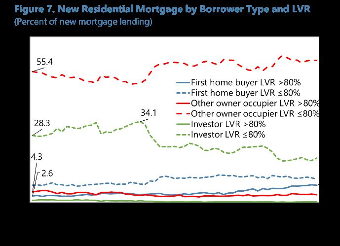
NEW ZEALAND
                     SELECTED ISSUES
September 5, 2019

                        Approved By                Prepared by Geoff Bannister, Dirk Muir, and Yu Ching Wong
                        Asia and Pacific           (all APD), with additional inputs from Ioana Hussiada and
                        Department                 assistance from Nadine Dubost (both APD).

                       CONTENTS
                    TRADE NET MIGRATION AND AGRICULTURE: INTERACTIONS BETWEEN EXTERNAL
                    RISKS AND THE NEW ZEALAND ECONOMY __________________________________________ 3
                    A. The Interaction of External Risks and Linkages in New Zealand _______________________ 3
                    B. Spillovers from a Growth Slowdown in China _________________________________________ 6
                    C. Spillovers from the Interplay of Net Migration and the Australian Economy _________ 14
                    D. Spillovers to New Zealand’s Agriculture Sector ______________________________________ 18
                    E. Conclusions __________________________________________________________________________ 20

                    References _____________________________________________________________________________ 21

                    BOX
                    1. ANZIMF – The Australia-New Zealand Integrated Monetary and Fiscal Model ________ 4

                    FIGURES
                    1. New Zealand’s Agricultural Exports ___________________________________________________ 3
                    2. New Zealand’s Services Exports _______________________________________________________ 3
                    3. Growth Slowdown in China – Outcomes in China _____________________________________ 7
                    4. Growth Slowdown in China – Spillovers to New Zealand ______________________________ 8
                    5. Growth Slowdown in China – Net Migration Effects in New Zealand _________________ 10
                    6. Growth Slowdown in China with Various New Zealand Policy Options _______________ 12
                    7. Growth Slowdown in China with Fiscal Stimulus in Different Economies _____________ 13
                    8. Growth Slowdown in Australia – Outcomes in Australia ______________________________ 14
                    9. Growth Slowdown in Australia – Spillovers to New Zealand _________________________ 16
                    10. Growth Slowdown in Australia – Net Migration Effects in New Zealand ____________ 17
                    11. Agriculture Sector Risk Scenarios ___________________________________________________ 19

                     TABLE
                    1. Trade Patterns in ANZIMF____________________________________________________________ 15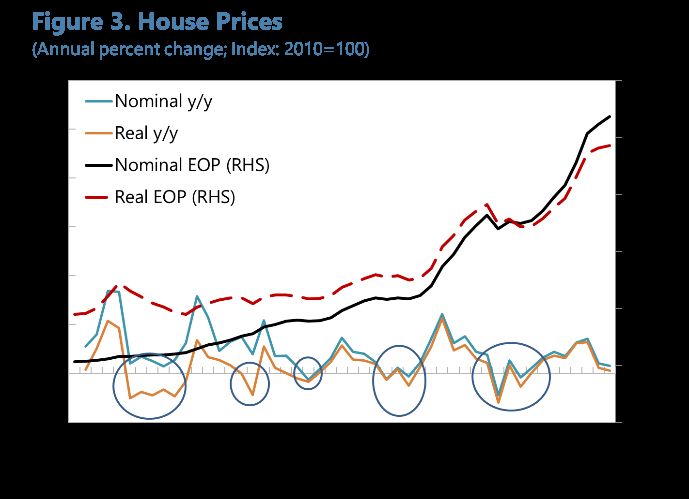
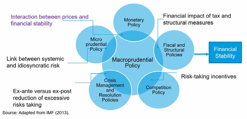
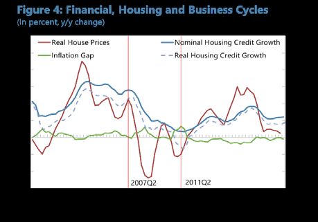
NEW ZEALAND

ANNEXES
I. Key Assumptions Underlying the Simulations_____________________________________________________ 22
II. New Zealand’s Fiscal Multipliers in ANZIMF ______________________________________________________ 25

QUANTIFYING CONSUMPTION-EQUIVALENT WELFARE IN NEW ZEALAND ___________________ 27

References__________________________________________________________________________________________ 33

FIGURES
1. Consumption-Equivalent Welfare vs. Income, 2017 ______________________________________________ 29
2. New Zealand, Welfare Index in 2017 _____________________________________________________________ 29
3. Progress in Welfare Over Time __________________________________________________________________ 30

TABLES
1. Mapping Consumption-Equivalent Welfare (CEWS) Indicators Into Living Standards
  Framework (LSF) __________________________________________________________________________________ 28
2. Welfare Indicators, 2017 _________________________________________________________________________ 30
3. Growth of Welfare, Income, and Components, 2007-2017 _______________________________________ 31

INTERACTION BETWEEN MONETARY POLICY AND FINANCIAL STABILITY IN NEW
ZEALAND __________________________________________________________________________________________ 35
A. Introduction _____________________________________________________________________________________ 35
B. A Review of the Debate on Monetary Policy and Financial Stability ______________________________ 36
C. Macroprudential Policy, Financial Stability, and Monetary Policy_________________________________ 38
D. Monetary Policy and Financial Stability in New Zealand _________________________________________ 39
E. Conclusions ______________________________________________________________________________________ 44

References__________________________________________________________________________________________ 45

BOXES
1. Debate on the Role of Monetary Policy in Achieving Financial Stability __________________________ 37
2. Macroprudential Policy Framework ______________________________________________________________ 42

FIGURES
1. Monetary Policy and Financial Stability To Lean or Not to Lean and their Trade-offs ____________ 38
2. Achieving Financial Stability: Relationship between Macroprudential and Other Policies_________ 39
3. House Prices _____________________________________________________________________________________ 40
4. Financial, Housing and Business Cycles __________________________________________________________ 40
5. Policy Rates, Inflation Gap, and Output Gap _____________________________________________________ 40
6. Policy Rates, House Prices, and Household Debt _________________________________________________ 40
7. New Residential Mortgage by Borrower Type and LVR___________________________________________ 42
8. Existing Residential Mortgage Lending___________________________________________________________ 42

TABLE
1. Housing Price Cycles, 2000-2018 _________________________________________________________________ 41

2    INTERNATIONAL MONETARY FUND
NEW ZEALAND

TRADE, NET MIGRATION AND AGRICULTURE:
INTERACTIONS BETWEEN EXTERNAL RISKS AND THE
NEW ZEALAND ECONOMY1
A. The Interaction of External Risks and Linkages in New Zealand

1.      As a small open economy, New Zealand is vulnerable to external risks, a concern at a
time when downside risks to the global economy have increased. The risks of greatest concern
are those that would involve New Zealand’s key external linkages – trade in tourism and education
services, trade in agricultural goods, and external wholesale funding of its banks – or key trading
partners and markets – Australia, China, and global markets for agricultural goods. In this paper, the
external risks related to trade are examined, using the Australia-New Zealand Integrated Monetary
and Fiscal Model (ANZIMF), a version of GIMF, the IMF’s Global Integrated Monetary and Fiscal
model (Box 1).

2.      This paper considers three channels for New Zealand’s external linkages.
     1) New Zealand is a large-scale agricultural exporter of agricultural goods, especially dairy
        products (Figure 1). Agricultural exports account for over 13 percent of New Zealand’s GDP.
     2) New Zealand is a large exporter of tourism and education services, referred to hereafter as
        services. While it has a diverse clientele for both, its largest relationships are with Australia
        and China (Figure 2). Export links with Australia tend be strongest for services, while those
        for China tend to involve more agricultural goods.

 Figure 1. New Zealand’s Agricultural Exports            Figure 2. New Zealand’s Services Exports
 (Percent of New Zealand GDP)                            (Percent of GDP)

 Sources: StatsNZ, UN COMTRADE, and IMF staff            Sources: OECD.stat EBOPS 2010 database, StatsNZ,
 calculations.                                           and IMF staff calculations.

1
  Prepared by Dirk Muir (APD). The chapter benefited from valuable comments by the Treasury of New Zealand and
participants at a joint Treasury and Reserve Bank of New Zealand seminar.

                                                                       INTERNATIONAL MONETARY FUND           3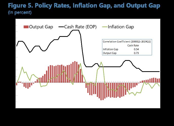
NEW ZEALAND

       3) Net immigration is a third source of external linkages, which has become increasingly
          important in the past five years. A novel feature of this paper is to consider the additional
          impacts from potential changes in net migration arising from the risks under consideration.
          Net migration into New Zealand, while slowing, is still near record-high levels. It is in part
          driven by external factors. Students coming to school in New Zealand (many from Australia
          and China) are staying as permanent residents afterwards. Australia also accounts for other
          migration flows – not just of Australian citizens but also returning New Zealand citizens who
          left when the domestic economy was relatively weaker.

         Box 1. ANZIMF – The Australia-New Zealand Integrated Monetary and Fiscal Model

    ANZIMF is an annual, multi-region, micro-founded general equilibrium model of the global
    economy. It is based on the IMF’s Global Integrated Monetary and Fiscal model (GIMF), with supporting
    documentation that is broadly applicable to ANZIMF (Kumhof and others, 2010, and Anderson and others,
    2013). Structurally, each country/regional block is close to identical, but with potentially different key
    steady-state ratios and behavioral parameters (Table 1). This exercise focuses on New Zealand.
               ANZIMF Expenditure Accounts Calibration                                Consumption dynamics are driven
                                        New                        Rest of   United   by higher-income, saving
                                       Zealand Australia   China    Asia     States   households and non-saving,
     Share of Global GDP (Percent)      0.23      1.7      15.1     14.6      24.4    lower-income households. Saving
                                                                                      households face a consumption-
     Domestic Demand (Percent of GDP)
                                                                                      leisure choice, based on the
     Household Consumption              60.4      55.1     54.5     58.7      62.0
     Private Investment                 16.3      21.3     25.0     21.0      18.2
                                                                                      overlapping generations (OLG)
     Government Absorption              23.3      23.6     20.5     23.0      19.8    model of Blanchard (1985), Weil
          Consumption                   19.5      19.8     13.5     20.0      16.3    (1989) and Yaari (1962). Households
          Investment                     3.8      3.8       7.0      3.0      3.5     treat government bonds as wealth
     Trade (Percent of GDP)
                                                                                      since there is a chance that the
     Non-Commodity Exports              14.1      19.1     17.4     26.3      13.7    associated tax liabilities will fall due
          Goods                         11.7      17.6     17.0     24.2      12.8    beyond their expected lifetimes
          Services                       2.4      1.5       0.4      2.1      0.9     making the model non-Ricardian.
     Non-Commodity Imports              -21.0    -25.1     -17.3    -25.5    -13.7    The long-term real global interest
          Goods                         -19.4    -23.1     -16.5    -23.6    -13.2    rate, therefore, is endogenous and
          Services                       -1.6     -2.0     -0.8     -1.9      -0.5    equilibrates global savings and
     Net Agriculture                    11.0      1.9       0.1     -1.2      0.3     investment. The real exchange rate
     Key Parameters                                                                   serves to adjust each country’s
     Percent share of LIQ households     25       25        25       40        25     saving position (its current account
                                                                                      and associated stock of net foreign
     Note 1: "Services" includes tourism and education services.                      assets) relative to the global pool.
     Note 2: "Goods" includes consumption, investment, and intermediate               Non-saving, lower income
     goods and other services.                                                        households must consume all their
     Sources: IMF staff calculations; IMF’s World Economic Outlook and                income each year, amplifying the
     Direction of Trade Statistics databases; U.N. Comtrade; OECD.Stat National       model’s non-Ricardian properties in
     Accounts Database.                                                               the short term.
     Private investment relies on the Bernanke-Gertler-Gilchrist (1999) financial accelerator. Investment
    cumulates to the private capital stock for tradable and nontradable firms, which is chosen by firms to
    maximize their profits. The capital-to-GDP ratio is inversely related to the cost of capital, which is a function

4       INTERNATIONAL MONETARY FUND
NEW ZEALAND
Box 1. ANZIMF – The Australia-New Zealand Integrated Monetary and Fiscal Model
(concluded)
of depreciation, the real corporate interest rate, the corporate income tax rate, and relative prices, and an
endogenously determined corporate risk premia.
Government absorption consists of exogenously determined spending on consumption goods and
infrastructure investment. Both affect the level of aggregate demand. Spending on infrastructure
cumulates into an infrastructure capital stock (subject to a constant but low rate of depreciation). A
permanent increase in the infrastructure capital stock permanently raises economy-wide productivity.
Trade is tracked bilaterally between all regions. There are flows for goods, services, and agricultural
goods, and they react to demand, supply and pricing (i.e., the terms of trade and bilateral real exchange
rates) conditions. Agricultural goods trade, and its related demand and supply equations, are based on a
broad array of products, as New Zealand has strong exports for dairy products, meat, and fruit.
The nominal side of the economy depends on implicit Phillips’ curves and monetary policy. The core
price is the consumer price index (CPI), while relative prices mimic the structure of the national expenditure
accounts. There is also wage inflation, which is implicitly a key driver for CPI inflation. In the short term, the
nominal side of the economy is linked to the real side through monetary policy, which is conducted under a
CPI inflation targeting regime, where with an interest rate function returns expected inflation to target over
several years.
Fiscal policy is driven by a sufficiently detailed government sector that can reproduce simplified fiscal
accounts for each country. Fiscal policy aims to maintain a debt target (expressed in flow space as a deficit
target), using at least one of seven policy instruments available in the model. On the spending side, they are
government consumption, infrastructure spending, general lumpsum transfers to all households (such as
pensions, aged care provisions, unemployment insurance) and lumpsum transfers targeted to LIQ
households (such as welfare, certain pensions). On the revenue side, the instruments are taxes on
consumption (the goods and services tax, GST), personal income (PIT) and corporate income (CIT).
Relative to standard versions of GIMF, this model contains sectors for agriculture and for services.
The data definition for the agriculture sector in this application covers all agricultural goods, but the focus
for New Zealand is on dairy with significant contributions from meat (lamb and beef) and fruit (kiwi fruit).
Similarly, the definition of services is restricted to tourism (mostly travel, accommodation, and food services)
and education (mostly travel and correspondence courses).
The agriculture sector. The U.S. dollar global agriculture price is determined when producing countries sell
in a global market, from which all countries then compete for their demands based on price. Countries
produce agricultural goods from their endowment. Supply moves in tandem in the short term with the gap
between the current and medium-term average global price and reacts (optionally) to demand-driven long-
term changes in the global price. Both the short- and long-term price elasticities of supply are 0.40. Net
export flows are explicitly tracked, although it is possible from the structure of the model to deduce the
bilateral flows. Agricultural goods are part of consumption and inputs to both tradable and non-tradable
intermediate goods production (much more for tradables).
The services sector. Services are produced from tradable and nontradable goods. They are priced as an
input for consumption in New Zealand or exported to be consumed by foreigners. Services are exclusively
part of consumption, and their demand vis-à-vis consumption goods is relatively inelastic. Consumption of
services is a combination of services provided domestically or abroad. This allows for a final price of services
that will enter the CPI, much as consumption services combines with the consumption of goods to define
final household consumption.
INTERNATIONAL MONETARY FUND 5NEW ZEALAND
3. This paper considers how external risks affect New Zealand through the three spillover
channels. 2 The components and magnitudes of the risk scenarios are illustrative only. Their results
are presented relative to a baseline forecast consistent with the IMF’s World Economic Outlook. The
risk scenarios address three configurations of spillovers to New Zealand:
• Section B: Spillovers through all three channels, by considering a growth slowdown in China. It
includes exacerbating impacts from net migration and also considers potential roles and
interactions for New Zealand’s monetary and fiscal policies.
• Section C: Spillovers through the net migration channel, by considering an illustrative growth
slowdown in Australia.
• Section D: Spillovers from lower global agricultural prices caused by demand or supply factors,
contrasted with impacts from domestic supply factor.
Section E concludes.
B. Spillovers from a Growth Slowdown in China
4. Global trade tensions could result in a broad-based growth slowdown in China. This
risk scenario considers the possibility that global trade tensions could disrupt the ongoing structural
reform process. In that case, China’s real GDP would be significantly lower than expected under
current baseline forecasts, along with most components of GDP. However, exchange rate and terms
of trade adjustments would mitigate the impact on New Zealand’s GDP, although domestic demand
would contract.
A Growth Slowdown in China 3
5. China would experience substantially weaker real GDP growth under this scenario
(Figure 3). 4 Real GDP growth would be about 1 percentage point lower than in the baseline in the
short term, and about 0.6 percent lower for nine years. In the long term, the level of real GDP would
be 11.9 percent lower relative to the baseline. Two-thirds of the decline would be from lower
productivity, which leads to higher production costs and lower production capacity compared to the
baseline. China’s goods would be more expensive and would experience reduced foreign demand.
Inflation in tradable goods prices would be even weaker than before, being 1.0 percent lower by the
third year, and would only return to baseline after ten years. Lower inflation in China would result in
2
The external risk scenarios are quantified in detail in Annex I.
3
This scenario is derived from previous scenarios focused on China (Dizioli and others 2016) and Australia (Karam
and Muir 2017)
4
The growth slowdown in China is based on four shocks. The trade tensions are assumed to result in lower
productivity growth of about 0.5 percent per year for 10 years, reducing economy-wide productivity levels by
5 percent in the long term. At the same time, firms would face higher risk premiums, an increase of 0.5 percentage
points relative to baseline. House prices in the major urban centers would fall by 10 percent over two years. Demand
for imported agricultural goods would decline by about 0.5 percent per year, summing up to levels that are 9 percent
lower in the long term, as household preferences would be shifting to local products.
6 INTERNATIONAL MONETARY FUNDNEW ZEALAND
a negative inflation impulse to countries that import substantial quantities of Chinese goods, such as
New Zealand.
Figure 3. Growth Slowdown in China – Outcomes in China
(Deviations from WEO-consistent forecasts)
Note: The bar marked “SS” is the steady-state value.
Source: IMF staff calculations.
6. Household consumption would be considerably lower in this scenario. The decline in
house prices would decrease household wealth, while the lower productivity would reduce firms’
labor demand and, consequently, labor income, wealth, and consumption. Consumption growth
would be around 0.2 to 0.5 percentage points weaker than that of real GDP growth. Imports would
INTERNATIONAL MONETARY FUND 7NEW ZEALAND
also be lower, including imports of agricultural goods. The latter would result in lower global prices
for agricultural goods of almost 1 percent on impact and of 2.1 percent in the long term.
Figure 4. Growth Slowdown in China – Spillovers to New Zealand
(Deviations from WEO-consistent forecasts)
Note: The bar marked “SS” is the steady-state value.
Source: IMF staff calculations.
Spillovers to New Zealand
7. New Zealand would experience strong spillovers through trade channels (Figure 4). The
China-led fall in global agricultural prices would reduce the value of New Zealand’s production,
8 INTERNATIONAL MONETARY FUNDNEW ZEALAND
although lower prices would also shore up foreign demand outside China and New Zealand. A real
depreciation of the New Zealand dollar would mitigate the impact on exports over time. New
Zealand’s tourism and education exports would be 1.6 percent lower in the short term, for example,
but would decline by only 1.0 percent in the long term. The impact on agriculture and services
would be a wealth shock, and lead to a depreciated REER. Therefore, while goods exports would be
1.1 percent longer in the short term, goods exports would be 0.5 percent higher in the long term.
8. Economic activity would contract in the short term but would return to baseline in the
long term because of expenditure switching. The lower agricultural goods prices lower New
Zealand’s wealth and consumption, with the latter being 0.9 percent lower relative to baseline in the
long term. But given the behavior of exports, real GDP would contract by only 0.2 percent on impact
and be broadly unchanged relative to baseline in the long term.
How Lower Net Migration Could Exacerbate the Negative Impact on New Zealand
9. A growth slowdown in China could have the additional impact of reducing Chinese
student migration into New Zealand (Figure 5). A part of New Zealand’s services exports is
consumed in the country by temporary residents, namely exports of education services. In recent
years, this type of export has also contributed to increases in net migration into New Zealand
because students obtain work permits after graduation. Here, the net migration of Chinese students
is assumed to decline in line with the economic slowdown. The combination of lower consumption
in China and a shift in preferences toward domestically produced goods and services might well
result in fewer Chinese students attending school in New Zealand. This would not only reduce
services exports but could also mean fewer students remaining in New Zealand after graduation.
Currently, 17 percent of net migration comes from China in New Zealand. In the scenario below, it is
assumed New Zealand’s population is 0.1 percentage points lower per year for 10 years –
approximately 40 percent of the share of New Zealand’s net migration inflow coming from China.
10. The shock to net migration would operate through its impact on labor supply. It would
decrease the productive capacity of New Zealand and increase wage pressures. Given the lower
long-term labor supply, demand for capital would be less, so investment would be 0.2 (short term)
to 0.7 percent (long term) weaker relative to the scenario without the net migration effects. Wealth
would be lower, leading to household consumption being 1.8 percent lower instead of 0.9 percent.
Pressures from consumption and investment would reduce imports, decreasing the short-term
current account deficit before the long-term re-equilibration from the change in the REER.
11. The fall in net migration would exacerbate the negative spillovers to New Zealand
from China. Real GDP would now be 0.7 percent lower than baseline in the long term. Short-term
losses in the economy would be confined largely to the domestic sector. In the long term, the
external sector would not be as strong, as the REER would depreciate less (only 0.9 percent) because
of stronger real wages relative to the case without changes net migration. Services exports would be
1.6 percent lower relative to baseline, compared to 0.7 percent under the case without changes in
net migration.
INTERNATIONAL MONETARY FUND 9NEW ZEALAND
Figure 5. Growth Slowdown in China – Net Migration Effects in New Zealand
(Deviations from WEO-consistent forecasts)
Note: The bar marked “SS” is the steady-state value.
Source: IMF staff calculations.
The Interaction of Monetary and Fiscal Policy
12. A need for a fiscal policy response to an economic downturn in New Zealand is
becoming more likely than it has been in the past. The global risk profile is increasingly tilted to
the downside, at a time when the Reserve Bank of New Zealand’s (RBNZ) policy rate is already at a
low of 1 percent. If a major risk realized, the effective lower bound (ELB) on nominal interest rates
10 INTERNATIONAL MONETARY FUNDNEW ZEALAND
might be more likely to become a constraint on monetary policy. This section considers the effects
of a fiscal policy response to a slowdown in China with the policy rate at the ELB. The effects on New
Zealand would be relatively small if the RBNZ could cut the policy rate but much larger if it could
not (Figure V.1, blue versus red lines).
13. The effectiveness of a fiscal policy response would depend on the instruments used.
Depending on the instruments, the multipliers of the discretionary fiscal policy response would be
different. Two options at the opposite end of the spectrum of the multipliers are considered below: 5
• Lower Multipliers, Quicker to Deploy: Increased government consumption spending and a
GST rate cut.
• Higher Multipliers, Slower to Deploy: Increased government infrastructure investment and
GST rebates targeted to lower-income households.
Each pair of fiscal instruments would be changed by 0.5 percent of GDP relative to their original
paths for five years (Figure 6, green solid and dashed lines). As aggregate demand increased and led
to inflationary pressures, it is assumed that the monetary authority would not increase the overnight
cash rate even if inflation were to enter its target range in later years.
14. Both forms of fiscal stimulus would have the same qualitative effects. The additional
stimulus would push up inflation between 0.5 to 0.8 percentage points by the fifth year, thereby
reducing the real interest rate and stimulating the economy. It would also increase the government-
debt-to-GDP ratio, but by a manageable amount – only between 2.0 to 2.5 percent of GDP after
5 years. This is lower than what the cumulation of the deficits over the same period would seem to
imply at first consideration, because the stronger nominal growth provided by the stimulus would
increase the denominator of debt-to-GDP ratio relative to baseline.
15. In the case of the lower-multiplier fiscal stimulus, there would be a multiplier for real
GDP of 0.7 on impact. Real GDP would peak at 1.0 percent higher in the fifth year, relative to the
growth slowdown in China constrained by the ELB and no additional fiscal policy response.
Government spending would automatically increase aggregate demand. The temporary cut in the
GST rate would only increase consumption for lower-income, non-saving households. Higher-
income saving households consume smoothly from their stock of wealth, so the GST rate cut would
add little to household wealth and have no discernible effect on households’ level of consumption.
16. In the case of the higher-multiplier fiscal stimulus, there would be a multiplier for real
GDP of 1.1 on impact. Real GDP would peak at 1.6 percent higher in the fifth year, relative to the
growth slowdown in China constrained by the ELB and no additional fiscal policy response. Public
infrastructure investment, besides increasing aggregate demand, would increase productivity over
the medium-to-long term. This would encourage more short-term private investment and increase
the economy’s productive capacity for an extended period. A larger share of a targeted GST rebate
5
Annex II discusses the multipliers from the seven fiscal instruments available in ANZIMF and orders them from
highest to lowest.
INTERNATIONAL MONETARY FUND 11NEW ZEALAND
would likely be spent compared to a general GST rate cut, as it would affect only households that
would benefit strongly from such a rebate. There would be the risk that infrastructure investment
could not be increased as rapidly as depicted here.
Figure 6. Growth Slowdown in China with Various New Zealand Policy Options
(Deviations from WEO-consistent forecasts)
Source: IMF staff calculations.
12 INTERNATIONAL MONETARY FUNDNEW ZEALAND
17. New Zealand’s openness would mean that either fiscal stimulus package would
effectively induce a “fiscal devaluation.” The REER would depreciate between 0.4 and 0.6 percent
more than the case without fiscal stimulus. A fiscal devaluation would stimulate the economy
through the export channel.
18. In both cases, there would be a fair degree of leakage to abroad from the fiscal
stimulus. In New Zealand’s open economy, a significant portion of the fiscal stimulus would be
spent on imports. There would be a higher current account deficit (higher imports for consumption
and investment, or conversely, higher investment and government dissaving) of between 0.2 and 0.3
percentage points of GDP. Other more-closed economies might have higher multipliers from the
same package, and smaller increases in their current account deficits.
19. The effects of New Zealand’s fiscal stimulus would be reinforced if there was to be
simultaneous fiscal stimulus elsewhere in Asia and Australia (Figure 7). The fiscal stimulus in
other economies would have some positive spillovers through trade channels, and further stimulate
aggregate demand. This is in turn, in the presence of monetary accommodation, would allow for a
lower real interest rate and greater REER depreciation, which would further stimulate aggregate
demand.
Figure 7. Growth Slowdown in China with Fiscal Stimulus in Different Economies
(Deviations from WEO-consistent forecasts)
Source: IMF staff calculations.
INTERNATIONAL MONETARY FUND 13NEW ZEALAND
C. Spillovers from the Interplay of Net Migration and the Australian
Economy
20. Because of New Zealand’s deep economic links with Australia, a growth slowdown in
Australia might have large impacts on New Zealand. This includes the Trans-Tasman Travel
Arrangement, which allows free movement of labor between the two countries. In any slowdown
originating in Australia, net migration could potentially play a large role – a factor not often
considered for many countries, given the unique relationship and patterns of population
movements between Australia and New Zealand over time.
Figure 8. Growth Slowdown in Australia – Outcomes in Australia
(Deviations from WEO-consistent forecasts)
Note: The bar marked “SS” is the steady-state value.
Source: IMF staff calculations.
14 INTERNATIONAL MONETARY FUNDNEW ZEALAND
A Growth Slowdown in Australia
21. In this illustrative scenario, Australia’s real GDP growth would be substantially weaker
(Figure 8). 6 Real GDP growth would be lower by about 3 percentage points on impact, and continue
to be negative, subtracting around 0.5 percentage points off growth for another 9 years, such that
real GDP would be 9.3 percent lower in the long term. Over 20 percent would be attributable to
lower population growth from lower net migration. Lower population and productivity would reduce
the productive capacity of the economy, and lead to higher marginal costs and inflation. Exports
would become more expensive to produce. This would induce the Reserve Bank of Australia (RBA) to
cut interest rates, and there would be a short-term 2 percent REER depreciation before being
reversed by the continuing negative productivity shock. Therefore, foreign demand would eventually
fall after its initial positive reaction to the short-term depreciation and help drive the REER to
appreciate by 4.3 percent in the long term.
22. Imports would weaken with the economy. Lower housing prices would subtract from
financial wealth, restricting consumption, reinforced by lower productivity and population. Demand
for tourism and education services would be reduced by 5.9 percent on impact, falling to 9.8 percent
lower, before settling at only 4.7 percent lower. Agricultural imports are much less important for
Australia than China, particularly from New Zealand, so the impact would only be around 0.2 percent
of GDP in the short term, approaching 0.3 percent in the long term.
Spillovers to New Zealand
23. To understand the spillovers to New Zealand, it is useful to compare its relationship
with Australia versus
Table 1. New Zealand: Trade Patterns in ANZIMF
China. The relative impacts
(Percent of New Zealand nominal GDP)
should reflect the
Category for New Zealand Australia China Global
magnitudes of the growth
Aggregate Exports 4.5 5.0 27.5
slowdowns under
Agriculture 1.2 2.6 13.4
consideration – that of
Tourism and Education Services 0.3 0.4 2.4
Australia (9.3 percent of
Goods and Other Services 3.0 1.9 11.7
GDP in the long term) would
Aggregate Imports 3.4 5.4 27.5
be less than that of China
Agriculture 0.5 0.1 2.4
(11.9 percent of GDP in the
Tourism and Education Services 0.2 0.4 2.0
long term). Spillovers would
Goods and Other Services 2.7 4.9 23.1
also reflect that trade
Sources: StatsNZ, UN COMTRADE, and IMF staff calculations.
linkages are stronger with
6
This growth slowdown in Australia is based on four shocks. There would be a slowdown in net migration, reducing
labor supply about 0.25 percent per year for 10 years. At the same time, there would be a negative shift in
expectations around the effects of new technology on the economy, resulting in permanently lower path for
productivity, also about 0.25 percent per for year for 10 years. Both factors would contribute to a 20 percent decline
in housing prices during the first two years, reducing household wealth and consequently consumption. All three
factors would contribute to higher perceived country risk for Australia, which would permanently increase the
country risk premium by 0.5 percentage points within a couple of years, further depressing investment.
INTERNATIONAL MONETARY FUND 15NEW ZEALAND
China than Australia. In the context of ANZIMF, the relationship is close to that in the data in 2016
(Table 2). Moreover, shocks emanating from China are more likely to move global prices than those
from Australia as China is more than nine times the size of Australia in terms of nominal U.S. dollar
GDP.
Figure 9. Growth Slowdown in Australia – Spillovers to New Zealand
(Deviations from WEO-consistent forecasts)
Note: The bar marked “SS” is the steady-state value.
Source: IMF staff calculations.
24. New Zealand’s exports would be lower (Figure 9). New Zealand’s services exports would
be about 0.4 percent lower (0.6 percent in the long term), much less than in the China growth
16 INTERNATIONAL MONETARY FUNDNEW ZEALAND
slowdown considered above, and in line with the composition of New Zealand exports. Similarly,
goods exports would be roughly 1.3 percent lower (0.4 percent in the long term). Net agricultural
exports would be broadly unchanged, because Australia has weaker demand for New Zealand
agricultural goods than China, and no significant impact on global agricultural prices, unlike China.
Figure 10. Growth Slowdown in Australia – Net Migration Effects in New Zealand
(Deviations from WEO-consistent forecasts)
Note: The bar marked “SS” is the steady-state value.
Source: IMF staff calculations.
INTERNATIONAL MONETARY FUND 17NEW ZEALAND 25. These factors would weaken the domestic economy and real GDP would be 0.1 percent lower in the short and long terms. The fall in exports would reduce productive capacity and labor demand. The depreciation would discourage imports of consumption and investment goods. Overall, consumption would fall by 0.6 percent. Because of weaker inflation from aggregate demand, monetary policy would provide some short-term stimulus with lower real interest rates. There would be a short-term 0.1 percent of GDP deterioration in current account. In the long term there would be little impact on the current account as there would be a rebalancing between the domestic and external sectors, facilitated by a REER that would be 0.2 percent lower on impact, and 0.4 percent lower in the long term. How Net Migration Could Improve Outcomes for New Zealand 26. The results presented above do not account for the unique net migration patterns between Australia and New Zealand, which could potentially offset the negative impacts on New Zealand (Figure 10). This can be illustrated by attributing 20 percent of Australia’s lower population growth to higher net migration to New Zealand, Real GDP would expand steadily at about 0.2 percent per year, reaching 2.0 percent higher than baseline in the long term. The short- term benefits would be confined largely to the domestic sector. However, the external sector would also benefit in the long term as productive capacity would expand beyond domestic demand needs. Consequently, the REER would depreciate by 1.5 percent relative to baseline (instead of 0.4 percent). However, there would be little effect on the agriculture sector, as it would still be operating at capacity. 27. The impacts would come from the net migration shock increasing labor supply. It would directly increase the productive capacity of New Zealand and reduce wage pressures. Moreover, investment would peak at 2.0 percent higher in the short term to build up the capital stock needed to complement labor and would stabilize at 1.6 percent higher in the long term. There would be increased household wealth and 2.2 percent higher consumption. Higher consumption and investment would stimulate imports, increasing the current account deficit by 0.5 percent of GDP (instead of only 0.1 percent of GDP). D. Spillovers to New Zealand’s Agriculture Sector 28. New Zealand’s agriculture sector faces external risks that differ from those that could originate within the country. At the global level, a decrease in agricultural prices is considered, driven by either a permanent global (excluding New Zealand) supply increase or demand decrease of 10 percent for agricultural goods. These are contrasted against a supply decrease within New Zealand alone because of a sustained drought that lowers agricultural output by about 6 percent for 2 years before starting to recover. Global Risks from Both Supply and Demand 29. In the long term, the global price would be 2.7 percent lower from either a global supply increase or demand decrease (Figure 11, red and green lines). Overall, the long-term 18 INTERNATIONAL MONETARY FUND
NEW ZEALAND

effects would be similar between demand and supply shocks. In the short term, demand would
move sluggishly in response to higher supply, because it would need the lower price to clear the
market. Volume supplied would be assumed to be fixed in the long term. There would be short-term
supply changes in response to price changes. Since the global price must fall to re-equilibrate global
demand and supply, it would return demand to its baseline levels in the demand shock, whereas in
the positive supply shock it would lift demand to absorb the additional supply.

                              Figure 11. Agriculture Sector Risk Scenarios
                               (Deviations from WEO-consistent forecasts)

   Note: The bar marked “SS” is the steady-state value.
   Source: IMF staff calculations.

                                                                INTERNATIONAL MONETARY FUND       19
NEW ZEALAND 30. From the perspective of New Zealand, it only would experience a negative wealth shock from lower prices. In the short term, there may be some fall in production which could slow the fall in prices, but in the end, production would remain unchanged. Consumption would be weaker from the wealth effect – 0.5 percent in long term, but substantially more at 1.0 percent in the short term for the global supply shock. As households would need time to adjust their demand to lower wealth, they would also dissave in the short term. This would lead to a higher current account deficit by 0.5 percent of GDP and a REER depreciation of 1.2 percent under the global supply shock, but a nearly unchanged current account deficit and a REER depreciation of only 0.7 percent under the global demand shock. 31. There would be a long-term rebalancing of the domestic and external sectors. Long- term real GDP would be roughly unchanged, even after the initial short-term negative impact from the rapid current account deterioration in the global supply risk scenario. In the medium term, the REER depreciation would lead to higher non-agricultural exports of about 1.3 percent. How Domestically-Driven Risks Have Different Outcomes 32. For a domestically-driven risk such as a sustained drought in New Zealand, the outcomes would be markedly different (Figure 11, blue lines). One hand, the real GDP loss would be less, at only 0.4 percent on impact. However, the external sector would be much weaker from lower exports, with a higher current account deficit of 0.8 percent of GDP. There would be little impact on the global agricultural price. First, the drought is assumed to be only temporary, but more importantly, New Zealand is only a small global player, despite the large importance of agriculture in the domestic economy. Consequently, there would be little short-term mitigation from the 0.4 percent REER, depreciation, and there would be no significant external-domestic sector rebalancing. E. Conclusions 33. The current set of external risks have the potential to be extremely damaging to New Zealand, but two factors would likely mitigate the economic impact. First, the flexible exchange rate regime is a reliable shock absorber and automatic stabilizer from the perspective of real GDP, although it leads to a rebalancing between the domestic and external sectors in the economy. Second, net migration flows can reduce the negative impact of lower external demand under some circumstances, such as a growth slowdown in Australia. However, this is not a reliable stabilizer – the magnitude of net migration is subject to many factors, plus it can also reinforce negative impacts, such as the example of a growth slowdown in China. 34. Fiscal policy could also offset some of the short-term costs of adjustment. Fiscal policy can provide stimulus at relatively small and manageable cost to the already-low government debt to GDP ratio. Moreover, at the current juncture, fiscal policy might need to provide the bulk of policy support against negative shocks, as monetary policy might be ineffective if has become constrained by an effective lower bound on the monetary policy interest rate. 20 INTERNATIONAL MONETARY FUND
NEW ZEALAND

                                           References
Anderson, D., B. Hunt, M. Kortelainen, M. Kumhof, D. Laxton, D. Muir, S. Mursula, and S. Snudden,
       2013, “Getting to Know GIMF: The Simulation Properties of the Global Integrated Monetary
       and Fiscal Model,” International Monetary Fund, IMF Working Paper 13/55.

Bernanke, B., M. Gertler, and S. Gilchrist, 1999, “The Financial Accelerator in a Quantitative Business
       Cycle Framework,” in J. Taylor and M. Woodford, eds., Handbook of Macroeconomics, Volume
       1c, Amsterdam: Elsevier.

Blanchard, O., 1985, “Debts, Deficits and Finite Horizons,” Journal of Political Economy, 93: 223-47.

Bom, P. and J. Ligthart, 2014, “What Have We Learned from Three Decades of Research on the
       Productivity of Public Capital?” Journal of Economic Surveys, 28(5): 889-916.

Coenen, G., C. Erceg, C. Freedman, D. Furceri, M. Kumhof, R. Lalonde, D. Laxton, J. Lindé, A.
      Mourougane, D. Muir, S. Mursula, J. Roberts, W. Roeger, C. de Resende, S. Snudden, M.
      Trabandt, and J. in‘t Veld, 2012, “Effects of Fiscal Stimulus in Structural Models”, American
      Economic Journal: Macroeconomics, 4(1): 22-68.

Dizioli, A., B. Hunt, and W. Maliszewski, 2016, “Spillovers from the Maturing of China’s Economy”,
         International Monetary Fund, IMF Working Paper 16/212.

Karam, K. and D. Muir, 2018, “Australia's Linkages with China: Prospects and Ramifications of China's
       Economic Transition”, International Monetary Fund, IMF Working Paper 18/119.

Kumhof, M., D. Laxton, D. Muir, and S. Mursula, 2010, “The Global Integrated Monetary and Fiscal
      Model (GIMF) – Theoretical Structure” International Monetary Fund, IMF Working Paper
      10/34.

Weil, P., 1987, “Permanent Budget Deficits and Inflation,” Journal of Monetary Economics, 20: 393-
         410.

Yaari, M., 1965, “Uncertain Lifetime, Life Insurance, and the Theory of the Consumer,” Review of
        Economic Studies 32(2): 137-50.

                                                                  INTERNATIONAL MONETARY FUND           21
NEW ZEALAND
Annex I. Key Assumptions Underlying the Simulations
Key Model Assumptions for ANZIMF
1. All agents in the model (including households, firms and the fiscal and monetary authorities)
have perfect foresight.
2. The model has non-linearities in the financial accelerator, and potential for non-linearities in the
conduct of monetary policy by either encountering the zero-interest-rate floor (the effective
lower bound, ELB) or using monetary accommodation. Otherwise, the model is approximately
linear for small enough shocks.
3. All countries in ANZIMF have the same economic structures, differing only through their
parameterization and calibration.
4. The baseline calibration of ANZIMF is based on parameter values consistent with 2017 for the
great ratios to GDP such the capital stock, government debt and deficit, net foreign assets and
current account balance, and national accounts aggregates as well as trade flows, and 2016 and
2017 for services data.
5. The real exchange rate is a “jumper,” adjusting immediately in the first year to shocks, since it
follows the standard forward-looking, risk-adjusted uncovered interest rate parity condition
which equates the forward sum of Australia-international interest rate differentials with the one-
year in the exchange rate. However, there is no financial friction in the equation required to
bring the net foreign asset position to its steady state, as the net foreign asset position and its
dynamics solve endogenously as part of the OLG framework.
6. The agriculture sector is a global market with one global price.
7. China has a flexible exchange rate, with no capital controls. Capital controls are hard to model in
this context, and in the current environment, it is not clear that China would always impose them
if there were to be sudden movements in elements of the balance of payments.
8. There are no substantial financial market channels. ANZIMF only has a financial accelerator
(albeit using the full general equilibrium form with non-linearities) and assumes complete
domestic ownership of firms. All net foreign asset positions are denominated in U.S. dollars, in
all countries. Some financial channels could be mimicked by correlated, exogenously-specified
shocks.
9. The model is at an annual frequency, so degree of detail for some of the economy’s dynamics
are lost, particularly in the first year for investment.
Risk Scenario Assumptions
The risk scenarios result from shocks originating in China. Australia and the rest of the world interact
with spillovers that are either direct, via third countries, or via the global agricultural goods market.
22 INTERNATIONAL MONETARY FUNDNEW ZEALAND
Growth Slowdown in China
The scenario is composed of four separate shocks in China:
1. Lower productivity. Permanent 5 percent reduction in tradables and nontradables productivity.
Phased in as a -2 percentage points on productivity growth in year 1, and -1 percentage point
on growth in years 2 through 4.
2. Lower housing wealth. 10 percent decline on impact in year 1 in nontradable sector net worth,
to proxy for the permanent fall in the value of the housing stock.
3. Increased corporate risk premia. Permanent 0.5 percentage point increase in the corporate risk
premia for both tradable- and nontradable-producing firms. Phased in by year 4, declining from
an initial 2 percentage point increase on impact in year 1.
4. Lower agricultural goods demand. Permanent 5 percent reduction in demand for agricultural
goods. Phased in over 5 years.
Additional Net Migration Effect in New Zealand. There are permanently fewer migrants to New
Zealand from China. There is a 0.1 percent reduction in labor force growth for 10 years in New
Zealand, so that the New Zealand population is permanently 1.0 percent lower.
The Interaction of Fiscal and Monetary Policies in New Zealand. The overnight cash rate (the
RBNZ’s monetary policy rate, and ANZIMF’s short-term interest rate) is assumed to be unchanged
for 5 years and is expected each year to be unchanged until the end of the following year. There are
two different configurations of fiscal stimulus presented.
1. Higher-multiplier fiscal stimulus. 5-year, 0.25 percent of baseline GDP higher spending on
government infrastructure investment. 5-year 0.25 percent of baseline GDP rebate of GST
revenues to non-saving, lower-income households.
2. Lower-multiplier fiscal stimulus. 5-year, 0.25 percent of baseline GDP higher spending on
government consumption (wages, salaries and other operating expenses). 5-year cut in the
general GST rate such that government revenues are 0.25 percent of baseline GDP lower each
year.
Growth Slowdown in Australia
The scenario is composed of four separate shocks in Australia:
1. Lower net migration. Permanent 2.5 percent reduction in labor force. Phased in over 10 years
at 0.25 percentage points per year.
2. Lower productivity. Permanent 2.5 percent reduction in tradables and nontradables
productivity. Phased in over 10 years as a -0.25 percentage points per year.
3. Lower housing wealth. 20 percent decline on impact in year 1 in nontradable sector net worth,
to proxy for the permanent fall in the value of the housing stock.
4. Increased corporate risk premia. Immediate and permanent 0.5 percentage point increase in
the corporate risk premia for both tradable- and nontradable-producing firms.
INTERNATIONAL MONETARY FUND 23NEW ZEALAND Additional Net Migration Effect in New Zealand. There are permanently more migrants to New Zealand from Australia. There is a 0.26 percent increase in labor force growth for 10 years in New Zealand, so that the New Zealand population is permanently 2.6 percent higher. Agriculture Sector There are three different scenarios under consideration, each consisting of one shock: 1. Higher global agriculture supply. Immediate and permanent 10 percent increase in the global supply of agricultural goods, outside of New Zealand, by increasing the endowment (long-term supply curve). 2. Lower global agriculture demand. Immediate and permanent 10 percent reduction in the global demand for agricultural goods, outside of New Zealand, by reducing the consumer’s preference parameters for agricultural goods directly. 3. Drought in New Zealand. The supply of agricultural goods in New Zealand is reduced by 6.25 percent in years 1 and 2. It takes until year 6 for long-term supply to return to its previous levels. The short-term elasticity of agricultural goods supply is set to 0 in years 1 and 2, so that agricultural goods supply cannot respond to short-term price movements. The elasticity is increased gradually, returning to its original value by year 6. 24 INTERNATIONAL MONETARY FUND
NEW ZEALAND

          Annex II. New Zealand’s Fiscal Multipliers in ANZIMF
ANZIMF has seven fiscal instruments. On the spending side, they are government consumption,
government investment (infrastructure), lumpsum transfers to all households (such as pensions,
aged care provisions, unemployment insurance) and lumpsum transfers targeted to LIQ households
(such as welfare, certain pensions). On the revenue side, the instruments are taxes on consumption
(the goods and services tax, GST), personal income (PIT) and corporate income (CIT).

Fiscal multipliers can be computed from the change in real GDP in model simulations. ANZIMF
can be simulated with a change of one percentage point of baseline real GDP for two years for each
fiscal instrument, separately, to provide fiscal stimulus to the economy. Two assumptions for
monetary policy can be considered – either the RBNZ sets the overnight cash rate (OCR) to keep
inflation within the target range, or it accommodates the fiscal stimulus by leaving the OCR
unchanged for two years, so that monetary policy does not crowd out any of the fiscal expansion.

The fiscal instruments act on the economy through direct channels that then feed through the
rest of the economy. The only reduced-form effect is the productivity increase induced by an
increase in government infrastructure investment. This is calibrated using an estimate of the
elasticity of output with respect to infrastructure capital of 0.170 from Bom and Ligthart (2014).

    Table II.1. ANZIMF Fiscal Multipliers for New          Spending generally, but not always,
                      Zealand                              provides larger multipliers than tax
                                                           cuts (Table 3, top half). Government
                                   First Year Second Year  absorption multipliers are most effective,
  Normal Conduct of Monetary Policy                        as they enter the measurement of real
  Government Consumption              0.71        0.61
                                                           GDP directly, as well as stimulating the
  Government Investment               0.88        0.85     rest of the economy. Infrastructure
  Transfers to All Households         0.10        0.08     investment is more effective than regular
  Transfers to LIQ Households Only    0.38        0.35     government spending, as it also raises
  Goods and Services Tax              0.27        0.26     productivity. Lumpsum transfers
  Personal Income Tax                 0.24        0.23
                                                           targeted to liquidity-constrained (LIQ)
  Corporate Income Tax                0.18        0.21
                                                           households are third-most effective, as
  Overnight Cash Rate Held Fixed for Two Years             they are consumed in full immediately
  Government Consumption              0.83        0.67     by the targeted recipients. The GST is
  Government Investment               1.03        0.93     next, as it affects consumption behavior
  Transfers to All Households         0.12        0.09
                                                           of all households contemporaneously.
  Transfers to LIQ Households Only    0.45        0.39
                                                           PIT applies to all households, but saving
  Goods and Services Tax              0.31        0.29
  Personal Income Tax                 0.29        0.26     households smooth out the extra
  Corporate Income Tax                0.39        0.37     income as part of their large stock of
                                                           wealth; only the liquidity-constrained
 Source: IMF staff calculations.                           households spend it immediately. CIT
                                                           has even smaller effects, as its only
impact is on firms, who take a longer-term planning view. But coupled with an unchanging OCR, the

                                                                INTERNATIONAL MONETARY FUND       25
NEW ZEALAND CIT multiplier exceeds that of the GST and the PIT. Lumpsum transfers to all households have the smallest effect, as the lumpsum transfers to the saving households are smoothed out, in the same manner as a PIT cut. Moreover, lumpsum transfers are nondistortionary, unlike the distortionary PIT. When the RBNZ accommodates the fiscal stimulus, the multipliers are larger (Table 3, bottom half). Apart from the CIT, the ordering remains unchanged. The multipliers are roughly 15 to 20 percent larger (over 100 percent for the CIT) than with the normal conduct of monetary policy. The extent and ordering of the multipliers are generally consistent with other countries such as the United States, including other macroeconomic models (Anderson and others, 2013; Coenen and others, 2011). However, magnitudes are smaller, as New Zealand is a small, more open economy that will use a larger share of fiscal stimulus to buy foreign relative to domestic goods and services. 26 INTERNATIONAL MONETARY FUND
NEW ZEALAND

QUANTIFYING CONSUMPTION-EQUIVALENT WELFARE
IN NEW ZEALAND 1
1.       New Zealand presented its first Wellbeing Budget on May 30th, 2019. This represents
the culmination of substantial work over the past few years to integrate parts of the OECD
Framework for Measuring Well-Being and Progress into the New Zealand public sector. 2 The Budget
is part of a broader strategy embodied in the Treasury’s Living Standards Framework (LSF): to
consider a range of indicators and factors, beyond purely economic objectives, in policy decision
making. The framework focuses on “four capitals” (natural, human, social and financial/physical) that
promote wellbeing in 12 dimensions: civic engagement and governance; cultural identity;
environment; health; housing; income and consumption; jobs and earnings; knowledge and skills;
time use; safety and security; social connections; and subjective wellbeing.

2.      The Wellbeing Approach is part of a tradition that has sought to move “Beyond GDP”
to broader measures of economic welfare. Although income per capita is a common measure of
economic success, it has long been recognized to leave out important dimensions of both economic
achievement and wellbeing. The Stiglitz commission report (Stiglitz and others, 2009), for example,
proposed alternative indicators of economic performance and social progress. The IMF has recently
focused on the implications of income distribution (Ostry and others, 2014 and Clements and others,
2015), and gender (Kochhar and others, 2017). The Sustainable Development Goals (SDGs) at the
core of the post-2015 Development Agenda (United Nations, 2015), also recognize the many
dimensions of welfare including equality, education, gender and environmental protection.

3.      A common challenge for these approaches is to accurately measure multidimensional
welfare outcomes in a simple index. Summary measures that attempt to capture differences in
dimensions of welfare across countries have been developed, including the Human Development
Index (HDI) (UNDP, 2009), the Inclusive Development Index (IDI) (World Economic Forum, 2017), and
the Multidimensional Poverty Index (Alkire and Foster, 2011). More recently, baseline indices have
been developed to measure progress in the SDGs (Schmidt-Traub and others, 2017 and Sustainable
Development Solutions Network and the Bertelsmann Stiftung, 2018). However, these indexes often
aggregate the different indicators of wellbeing in an ad-hoc manner, making it difficult to know
exactly what is being measured, and how these change across countries or over time (Ravallion,
2012).

4.      One recent approach is to measure consumption-equivalent welfare. This approach
attempts to put an economic value (in terms of consumption) on different aspects of welfare, which
allows for a theoretically consistent aggregation to come up with a single index that can measure
differences in consumption-equivalent welfare across countries and over time. Jones and Klenow
(2016) developed an index that includes consumption itself, and life expectancy, leisure and

1
    Prepared by Geoffrey Bannister (APD).
2
 The OECD Framework for Measuring Well-being and Progress can be found at:
https://www.oecd.org/statistics/measuring-well-being-and-progress.htm

                                                                    INTERNATIONAL MONETARY FUND   27
You can also read