NON-LINEAR REGRESSION MODELS FOR BEHAVIORAL AND NEURAL DATA ANALYSIS
←
→
Page content transcription
If your browser does not render page correctly, please read the page content below
N ON - LINEAR REGRESSION MODELS FOR BEHAVIORAL AND
                                                                               NEURAL DATA ANALYSIS

                                                           Vincent Adam                                            Alexandre Hyafil
                                                           PROWLER.io                                        Centre de Recerca Matemàtica
                                                          Cambridge, UK                             Campus UAB Edifici C, 08193 Bellaterra, Spain
                                                                                                          and Center for Brain and Cognition
arXiv:2002.00920v1 [stat.AP] 3 Feb 2020

                                                     vincent.adam@prowler.io
                                                                                                   Universitat Pompeu Fabra, 08018 Barcelona, Spain

                                                                                               A BSTRACT
                                                   Regression models are popular tools in empirical sciences to infer the influence of a set of variables
                                                   onto a dependent variable given an experimental dataset. In neuroscience and cognitive psychology,
                                                   Generalized Linear Models (GLMs) -including linear regression, logistic regression, and Poisson
                                                   GLM- is the regression model of choice to study the factors that drive participant’s choices, reac-
                                                   tion times and neural activations. These methods are however limited as they only capture linear
                                                   contributions of each regressors. Here, we introduce an extension of GLMs called Generalized Un-
                                                   restricted Models (GUMs), which allows to infer a much richer set of contributions of the regressors
                                                   to the dependent variable, including possible interactions between the regressors. In a GUM, each
                                                   regressor is passed through a linear or nonlinear function, and the contribution of the different result-
                                                   ing transformed regressors can be summed or multiplied to generate a predictor for the dependent
                                                   variable. We propose a Bayesian treatment of these models in which we endow functions with Gaus-
                                                   sian Process priors, and we present two methods to compute a posterior over the functions given a
                                                   dataset: the Laplace method and a sparse variational approach, which scales better for large dataset.
                                                   For each method, we assess the quality of the model estimation and we detail how the hyperpa-
                                                   rameters (defining for example the expected smoothness of the function) can be fitted. Finally, we
                                                   illustrate the power of the method on a behavioral dataset where subjects reported the average per-
                                                   ceived orientation of a series of gratings. The method allows to recover the mapping of the grating
                                                   angle onto perceptual evidence for each subject, as well as the impact of the grating based on its
                                                   position. Overall, GUMs provides a very rich and flexible framework to run nonlinear regression
                                                   analysis in neuroscience, psychology, and beyond.

                                          Keywords regression · Gaussian process · neuroscience

                                          1     Introduction
                                          1.1   Regression models for data analysis

                                          Research questions in neuroscience and cognitive science often imply to empirically assess the factors that determine
                                          an observed neural activity or behavior in controlled experimental environments. Exploratory analyses on such
                                          datasets are typically performed using regression analyses - where the measured data (e.g. neural spike count, subject
                                          choice, pupil dilation) is regressed against a series of factors (sensory stimuli, experimental conditions, history of
                                          neural spiking or subject choices, etc.).

                                          A method of choice is the use of generalized linears models (GLMs [1]) where the dependent variable is predicted
                                          from a linear combination of the factors. More formally, GLMs are regression models from the input space X to the
                                          output space Y specifying a conditional distribution for the variable y ∈ Y given a linear projection ρ(x) = w> x
                                          of the input x ∈ X . ρ is called the predictor. The distribution of y|ρ(x) is chosen to be in the exponential family.
Figure 1: Example of GUM. Here 4 regressors (x1 , x2 , x3 , x4 ) are combined to generate a prediction for dependent
variable y. Each regressor is first passed through a linear function wi xi or non-linear function fi (xi ). Then regressors
are combined with a set of additions and multiplications to yield the predictor ρ(x), in this example ρ(x) = (f1 (x1 ) +
w2 x2 )f3 (x3 ) + w4 x4 . Finally, the expectation for dependent variable E(y) is computed by passing the predictor
through a fixed function g (the inverse link function). Inference corresponds to estimating the set of function (w, f )
based on a dataset (X, y).
This includes, for example, the Bernoulli, the Gaussian and the Poisson distribution that are used to deal with binary,
continuous and count data respectively. GLMs are very popular tools due to their good estimation properties (the
optimisation problem is convex and iterative estimation procedures converges rapidly), its ease of application and the
fact that it can accommodate for many types of data (binary, categorical, continuous) both for regressor and dependent
variable. The magnitude of the weight w is interpreted as indicating the impact of the corresponding factor on the
observed data, with a value of 0 indicating an absence of impact.
However, GLMs are intrinsically limited by their underlying assumption that the predictor linearly depends on the re-
gressors. In most situations, we expect regressors to have some non-linear impact onto the neural activity or behavior.
Generalized Additive Models P (GAMs) are a non-linear extension of GLMs where the linear predictor is replaced by
an additive predictor ρ(x) = k fk (x) where fk are functions from X → Y. Each fk usually depends on one or a
subset of dimensions sk ⊂ [1..dim(X )] of x (we will make this implicit in the rest of the article by using fk (x) instead
of fk (xsk )). Functions fk need to be constrained to have some quantifiable form of regularity (e.g. to be smooth),
both to make the problem identifiable and to capture a priori assumptions about these functions. Additivity in GAMs
introduces another form of identifiability, as functions are only defined up to an offset (i.e. replacing f1 by f1 + λ and
f2 by f2 − λ for any λ ∈ R does not change the model). For this reason, it is convenient to add one constraint
P on each
function (i.e. fi (0) = 0) and model the shift factor as an extra parameter c ∈ R to be estimated: ρ(x) = k fk (x) + c.
GAMs release the linearity constraint from GLMs that regressors are mapped linearly onto the predictor. However,
one may want to go beyond the additivity hypothesis and allow for non-linear interactions across the variables in the
regressor.
1.2 Generalized Unrestricted Model (GUM)
One way to achieve is to extend GAMs and add terms that are multiplications of functions to be learned. For
example, we would like to capture modelsP such as ρ(x) = f1 (x)f2 (x) + c, ρ(x) = (f1 (x) + f2 (x))f3 (x) + c,
ρ(x) = f1 (x)f2 (x) + f3 (x) + c or ρ(x) = i f1 (xi )f2 (xi )f3 (xi ) + c. We define a Generalized Unrestricted Model
(GUM) as a regression model composed of the following features: a set of functions or components fk defined
over the input space; a predictor function ρ(x) composed by summations and multiplications of the components; an
observation model y|ρ in the exponential family (Figure 1).
2The predictor can be constructed recursively using summations and multiplications over the functions. We will study
here a relatively general form, where the predictor is a sum of products of sums of GAM predictors (Figure 1):
X Y X
ρ(x) = fk(ijl) (x) (1)
i j≤Di l
All of the predictors presented in the previous section can be expressed in such form. As for GLMs and GAMs,
GUM regression consists in estimating the components fk given a dataset of regressor P X = (x(1) , .. . , x(N ) ) and a
(1) (N )
corresponding output y = (y , . . . , y ). We refer to a factor as a sum of functions l fk(ijl) (x) , and to a block
as the product of factors. The predictor is thus built as a sum of blocks. The dimensionality of each block Di is the
number of products within the block, i.e. the dimension of the multilinearity. A GAM can be seen as a GUM where
all the blocks have dimensionality 1.
1.3 Identifiability of GUMs
Using such a large class of models requires great care to ensure model identifiability. The summation of
functions induces a shifting degeneracy, while the multiplication of functions induces a scaling degeneracy:
f1 (x)f2 (x) = f1λ(x) (λf2 (x))
for any λ 6= 0. A general solution to this problem is to constrain all the functions to verify fk(ijl) (x0 ) = 0 for
some
P Q P
given x0 and to then add offsets cij ∈ R to the model, defining now ρ(x) = i j f
l k(ijl) (x) + c ij + c0 .
Equivalently, functions can be constrained to have mean 1 over a certain set of values We add some further
constraints on the offset depending on the model itself (see details in Appendix A). The examples of models provided
above will write as: ρ(x) = (f1 (x) + c11 )(f2 (x) + 1) + c0 , ρ(x) = (f1 (x) + f2 (x) + c11 )(f3 (x) + 1) + c0 or
ρ(x) = (f1 (x) + c11 )(f2 (x) + 1) + f3 (x) + c0 .
1.4 Bayesian treatment of GUMs
Recent progress in Bayesian statistics allows to derive algorithms to perform inference in such models that are both
accurate and scalable, meaning that they can be efficiently applied to the large datasets produced in neuroscience
today. Adopting the framework of probabilistic modelling [2, 3], we frame the model fitting task as probabilistic
inference and learning problems. To do so we treat the functions and parameters of the model as latent variables
and encode our a priori assumptions about these in the form of distributions (using Gaussian processes as priors
over functions [4]). Hyperparameters control the statistical properties of the functions, for example their smoothness
or perioditicity. Inference refers to estimating the functions f and offsets c of the model for a given value of the
hyperparameters, while learning refers to estimating the hyperparameters. Due to the model structure, the inference
problem is intractable and we resort to an approximate Bayesian inference technique called variational inference [5].
The remainder of this paper is structured as follows. Section 2 reviews the relevant background related to Gaussian
process inference and previous work in sparse approximations to GP models. In Section 3 the core methodology for
GUMs is presented. Implementation details and computational complexity of the method are covered in Section 4.
Section 5 is dedicated to a set of illustrative toy examples and a number of empirical experiments, where practical
aspects of GUM inference are demonstrated. Finally, we conclude the paper with a discussion in Section 7.
2 Methods
2.1 Probabilistic modelling and inference
2.1.1 General framework
We propose to tackle the problem of learning the functions and parameters of our regression models as probabilistic
inference problems. To do so we start by defining a joint distribution over the dependent variable y, and the parameters
θ given the regressors x, with density: p(y, θ|x) = p(y|ρθ (x))p(θ), where the first term is the exponential family
observation model inherited from the GLMs and p(θ) is an a priori distribution over the parameters capturing our
statistical beliefs or assumptions about their values. In the case of GUMs, parameters correspond to functions and
constraints, θ = {fk , ck }. Both the prior and likelihood may be parameterised by hyperparameters γ. As is the
case in most regression models, we will assume that conditioned on the parameters, the observations are statistically
independent, i.e. the likelihood factorizes across the data points: p(y|θ) = n p(y (n) |θ n ), where θ n ⊆ θ is the
Q
3subset of parameters on which observation y (n) depends.
We then propose to treat the inference problem as that of computing the posterior distribution over the parameters
which is defined as their conditional distribution given the observed data p(θ|y). The posterior density can be
expressed using Bayes’ rule as p(θ|y) = p(y|θ)p(θ)
R
p(y) . In this expression, p(y) = p(y, θ)dθ is the marginal likelihood
which is commonly used as a objective to select the value of the hyperparameters γ).
2.1.2 Gaussian processes: distributions over functions
Gaussian processes are commonly used as prior over functions [4] because they can flexibly constrain the space of ac-
ceptable solutions in non-linear regression problems. Formally, Gaussian processes are infinite collections of random
variables, any finite subset of which follows a multivariate normal (MVN) distribution. They are defined by a mean
function m and covariance function k. A sample from a GP defined on an index set X is a function on the domain
X . Given a list of points X ∈ X N and a GP sample f ∼ GP (m, k), the vector of function evaluations f (X) is an
associated MVN random variable such that f (X) ∼ N (m(X), K(X, X)), where m(X) is a vector of mean function
evaluations and K(X, X) is a matrix of all pairwise covariance function evaluations (K(X, X)ij = k(xi , xj )). The
covariance function may depend on some hyperparameters γ (the mean function can be too, although in most appli-
cations it is taken to be the zero function). For example, the classical Squared Exponential (SE) covariance function
defines covariance for real-valued data X = Rd based on two hyperparameters: length scale ` (which parametrises
the expected smoothness of the function) and variance β 2 (which parameterises the expected magnitude of the func-
0 2 2
tion) (kSE (x, x0 ) = β 2 e−|x−x | /2` ). As such, the covariance and mean functions define soft constraints over the
functions f (X) that fulfill two goals: make the functions f (X) identifiable, and formalizing assumptions about the
possible forms that f (X) may take (i.e. its smoothness).
2.1.3 Variational inference
Evaluating the posterior density p(θ|y) and the marginal likelihood p(y) is in general intractable for a GUM. We
therefore resort to perform approximate inference and focus on variational inference methods [5]. Variational inference
turns the inference problem into an optimisation problem by introducing a variational distribution over the parameters
q(θ) and maximising a lower bound L(q) to the log marginal evidence log p(y). This lower bound is derived using
Jensen’s inequality :
Z Z
p(y, θ) p(y, θ)
log p(y) = log dθ q(θ) ≥ q(θ) log = L(q) (2)
q(θ) q(θ)
The lower bound can be rewritten as
X
L(q) = Eq(θn ) log p(yn |θ n ) − KL[q(θ)|p(θ)], (3)
n
which is the form favored for actual implementations. The left-hand terms in the sum are the variational expectations
and require computing an expectation under the marginal distributions q(θ n ).
The gap in the inequality in Equation 2 can be shown to be log p(y) − L(q) = KL[q(θ)|p(θ|y)], where KL denotes
the Kullback-Leibler divergence between distributions. Hence, as q(θ) gets closer to the true posterior p(θ|y), the
bound gets tighter. In practice, one chooses the class of distribution Q such that optimising L(q) for q is tractable.
Once optimised, the optimal variational distribution q ∗ (θ) provides an approximation to the posterior and the bound
L(q ∗ ) provides an approximation to the log marginal likelihood.
The choice of the class Q is driven by two opposite goals: Q must be rich enough so that at the optimum, q ∗ captures
most important features of p(θ|y), but simple enough that L(q) is computationally efficient to evaluate for all q ∈
Q. When a finite dimensional parameter θ is endowed a prior distribution which is a multivariate normal (MVN)
distribution, a convenient choice for Q is the class of MVN distributions parameterised by a mean vection µq and a
covariance Σq , i.e. q(θ) = N (θ; µq , Σq ) [6]. In that case, computing the marginals q(θ n ) is straightforward and the
KL between two MVNs has a simple expression. The evaluation of the variational expectations in Equation 3 can be
evaluated in closed form or approximated using Gaussian quadrature or Monte Carlo methods [7].
When working with functions f (·) and using Gaussian Processes - infinite dimensional objects - as priors, an efficient
and scalable way to parameterise the variational distribution as a finite dimensional Gaussian Process expressed at
4some input z ∈ X M as follows:
q(f (·), f ) = p(f (·)|f (z) = f )q(f ),
where f = f (z), q(f ) = N (f ; µf , Σf ) is a MVN distribution and p(f (·)|f (z)) is the conditional prior process. q(f )
can be interpreted as an approximate marginal posterior on f (z). Choosing z = x is the classical variational treatment
of GPs but leads to a computational cost to evaluate L(q) that scales cubically with N , making the use of variational
inference prohibitively expensive for large datasets. Choosing z ∈ X M to be a set of pseudo-inputs (or inducing
points) of size M leads to the so-called sparse variational approach [8, 7, 9, 10] whose O(N M 2 + M 3 ) complexity
allows to scale variational inference with GPs to large datasets.
In order to enforce the necessary constraints that make the model identifiable, it is possible to force the posterior
processes to have a predictive mean at an input xc to be equal to yc . To do so we adjust the variational mean by a
y −Ep [f (xc )|f (z)=µf ]
scaled unit vector µf ← µf + δ1 such that Eq [f (xc )] = yc , where δ = c Ep [f (xc )|f (z)=1] . This is the method we
use in our examples.
2.1.4 Laplace approximation
The Laplace approximation provides an alternative MVN approximation q(θ) = N (θ; µq , Σq ) to the posterior p(θ|y).
This approximation is derived from a Taylor expansion of the log-joint density log p(θ, y) taken at the maximum a
posteriori parameters θ MAP = arg maxθ p(θ, y):
1
log p(θ, y) ≈ a + b(θ − θ MAP ) − (θ − θ MAP )T H(θ − θ MAP ) (4)
2
where a = log p(θ MAP , y), b = ∇θ log p(θ, y)|θ=θMAP = 0 by definition of θ MAP , and H =
−∇∇θ log p(θ, y)|θ=θMAP . H is a definite-positive matrix since it is the opposite Hessian of a function evaluated
at its maximum. The expansion leads to
a 1 MAP T MAP
p(θ|y) ∝ p(θ, y) ≈ e exp − (θ − θ ) H(θ − θ ) (5)
2
R
The constant of proportionality is obtained from the normalization constraint p(θ|y)dθ = 1, yielding the MVN
form p(θ|y) = N (θ; µq , Σq ) with µq = θ MAP and Σq = H −1 = [−∇∇θ log p(θ, y)|θ=θMAP ]−1 .
The Laplace approximation is a fairly simple procedure, as it only requires to find the maximum a posteriori param-
eters θ MAP , and to then compute the Hessian of the log-joint probability evaluated at θ MAP . The approximation is
increasingly better as the sample size n increases, as the true posterior becomes closer to a MVN distribution [3].
However the computational complexity of the method scales cubically with the number of data points.
2.2 Approximate inference for GUMs
We present two different approximate methods to treat GUMs: Laplace approximation and sparse variational inference.
For each method, we describe first how inference can be performed, i.e. how the posterior over the functions f and
offsets c can be approximated from a dataset, assuming fixed values of the hyperparameters for the different GPs.
Then, for each method, we describe how these hyperparameters can also be learned from the dataset.
2.2.1 Laplace approximation for GUMs
Inference For classical GP classification, the Laplace approximation follows by recognizing that the problem is
formally equivalent to a Bayesian GLM, where the parameters are the value of the GP at data points f = f (x), the
prior covariance is given by the GP evaluated at data points K(x, x) and the design matrix is identity [4]. Then the
MAP solution f MAP can be found iteratively using Newton-Raphson updates (the joint density is convex), and the
Hessian can be evaluated analytically. Computing the Laplace approximation for GUMs follows a similar path. The
derivation is quite lengthy, so we summarize here the main steps (details are provided in Appendix B).
First, a GUM can be turned into a Bayesian formulation of a generalized multilinear model [11, 12], as multiplications
of functions yield multilinear interactions of the parameters fk = fk (x). The constraints on fk added to remove
identifiability problems lead to removing one free parameter for each parameter set fk . The MAP solution is then found
by iteratively performing Newton-Raphson update on each dimension while leaving others parameters unchanged. For
example for a GUM ρ(x) = f1 (x)f2 (x), we update the value of f1 while leaving f2 unchanged, then we update f2
while f1 is unchanged, and loop until convergence. Each iteration increases the value of the joint density. Finally,
the covariance of the approximated posterior can be computed analytically by evaluating the Hessian of the log joint
density at the MAP parameters.
5Hyperparameter fitting For Laplace approximation we describe two different ways of fitting the hyperparameters
γ for the prior covariance functions Kij = Kij (γ ij ): cross-validation and generalized expectation-maximisation
[13].
In cross-validation, we split the dataset between a training set and a test set (possibly multiple times, as in K-fold
cross-validation). We infer the MAP estimate θ MAP using the training set only, then compute the cross-validated
log-likelihood (CVLL), i.e. the log-likelihood of the MAP parameters evaluated on the test set log p(y test |θ MAP ). The
gradient of the CVLL over the hyperparameters can be calculated analytically (see Appendix B.4.1). This allows to
run a gradient ascent algorithm which iterates between computing the MAP estimates for given hyperparameters and
then updating the hyperparameters to along the gradient to improve the CVLL score.
In expectation-maximisation,
R we used the approximated posterior q(θ) to update the lower bound on model evidence
L(q, γ) = q(θ) log p(y|θ, γ)dθ + const. The algorithm iterates between the expectation step (inference using
Laplace approximation) and the maximisation step where the lower bound is maximised with respect to the hyper-
parameters. Because both priors and posteriors are Gaussian, the lower bound can be expressed analytically and
maximised using gradient ascent. Note however that, because the posterior is not exact but approximated, the lower
bound is not guaranteed to increase at each expectation step.
2.2.2 Sparse variational approximation for GUMs
Inference Variarional inference has been been used to learn GLMs [14] and GAMs [15, 16]. In these settings, having
multiple functions, we need to specify a variational posterior over the functions and scalar parameters q(f1...K , c). We
follow [17] and assume it factorizes as
Y
q(f1...K , c) = q(f1...K , c) p(fk |fk (z k ) = fk ),
k
P
Mk
which means that posterior processes are only coupled through the inducing variables f1...K ∈ R k (Mk is the
number of inducing points for fk ).
We are left to characterize the finite density q(f1...K , c). We choose to parameterise it as a MVN distribution. A first
option is to parameterise it as fully coupled MVN distribution, which would capture the posterior coupling but would
also do so in a overparameterised
Q Q fashion. The other extreme would consist in a mean field approximation across term
q(f1...K , c) = k q(fk ) i q(ci ) which would under-estimate the posterior variances [3] and possibly bias learning
[18].
Q
We propose a parameterisation that preserves coupling across functions: q(f1...K , c) = q(f1...K ) i q(ci ), where we
let each factor be a MVN distribution. For each function we enforce q(fk (0)) = 0 using the method described in
Section 2.1.3.
Hyperparameter fitting When using variational inference, L(q) is used as a proxy to the log marginal likelihood and
can be optimized with respect to the hyperparameters γ as well as with respect to q, an approach akin to Expectation
Maximisation [3]. We here follow this approach: we iterate between maximizing L(q) over q with γ fixed (inference)
and maximizing L(q) over γ with q fixed (learning).
3 Results
3.1 Synthetic data
We first tested the ability of the different algorithms to infer the correct form of functions from synthetic data. We
generated Poisson observations y (E(y|ρ) = eρ ) from a simple GUM of the form ρ(x) = f1 (x1 )f2 (x2 ) + f3 (x3 )
and then applied our algorithms to fit the functions (f1 , f2 , f3 ) on the dataset (x, y). We chose f1 and f3 to be
functions of a closed interval [0, 2] and f2 to be periodic (of period π). This could correspond for example to
regressing the spiking activity of a neuron in visual cortex against the properties of visual stimulus defined by
its contrast and orientation: f1 (x1 ) would be the modulation of firing rate by contrast, f2 (x2 ) the orientation
selectivity, and f3 (x3 ) could be the fluctuation of neural excitability across time (with x3 being time). More
specifically, we defined f1 (x1 ) = exp(x1 /2) − 1, f2 (x2 ) = 1 + cos(2x2 + π/3) and f3 (x3 ) = − sin(x). For
0 2
estimation of f1 and f3 we used the standard Squared Exponential kernel KSE (x, x0 ) = β 2 exp − |x−x 2`2
|
with
650 observations 200 observations 500 observations
2 2 2
f1(x1)
1 1 1
0 0 0
0 1 2 0 1 2 0 1 2
2 2 2
f2(x2)
1 1 1
0 0 0
0 /2 0 0 /2 0 /2
0
0
f3(x3)
1 1
1
0 1 2 0 1 2 0 1 2
2 2 2
(X)
(X)
(X)
0 0 0
1 0 1 2 1 0 1 2 0 2
(X) (X) (X)
Figure 2: Estimated functions using Laplace method from GUM model with predictor ρ(x) = f1 (x1 )f2 (x2 )+f3 (x3 ).
Posterior distribution for each function fi is a Gaussian Process fi ∼ GP (mi , ki ). Solid black lines depict the
posterior mean function mi (x), dotted lines depict the posterior standard error. Red lines depict the ground truth, i.e.
the functions that were used to generate the dataset. Different columns represent different sizes for the dataset used to
estimate the functions (50, 200 or 500 observations).
the value of the hyperparameters β = 1 and length scale ` = 0.1. For f2 we used the standard periodic kernel
Kper (x, x0 ) = β 2 exp − 2 sin2 ( Tπ |x − x0 |)/`2 , with hyperparameters β = 1, ` = π/20 and period T = π.
We report the inferred functions and the resulting predictors for both methods in Figure 2 (Laplace method) and
Figure 3 (sparse variational inference) which show the functions are correctly recovered, even for small sized. The
reconstruction error is compared between the different sizes of the dataset (N = 50, 200, 500 observations) in Figure 4.
Using priors over the functions implies that the estimator will be biased (towards zero), and that the bias will be larger
for smaller datasets. In practice, however, such shrinking effect was very small for N = 200, 500, and was only
pronounced for the smaller sample size (N = 50) for the estimation of f2 . As expected, all three functions were more
accurately estimated for larger sample sizes. Both methods achieve similar regression performance as measured by the
root mean squared error (RMSE) on the predictor, which decreases as the number of observations grows (Figure 5). In
terms of computing however, the sparse variational method clearly outbeats the Laplace method for large sample size
(from N = 500). For the Laplace method, we also report the reconstruction error between the true function fi and
estimated function fˆi as erri =< (fi (xi ) − fˆi (xi ))2 >xi .
3.2 Experiments: psychophysical data - perceptual decision study
The very flexible functional forms of GUMs makes them applicable to a wide range of problems in psychophysics,
neuroscience and beyond. We illustrate GUMs on experimental data from a study using a classical evidence accumu-
lation paradigm [19].
A classical problem in cognitive neuroscience is to understand how humans integrate evidence from multiple sources
of information to make decisions [19]. One embodiment of this problem is the study of how this integration happens
across time given a temporal sequence of stimuli, such as oriented gratings [20]. In such paradigms, subjects report
750 observations 200 observations 500 observations
1 1 1
f1(x1) 0 0 0
0 1 2 0 1 2 0 1 2
2 2 2
f2(x2)
1 1
0 0 0
0 /2 0 /2 0 /2
0 0 0.0
f3(x3)
0.5
1 1 1.0
0 1 2 0 1 2 0 1 2
2 2 2
(X)
(X)
(X)
0 0 0
2
1 0 1 2 1 0 1 2 0 2
(X) (X) (X)
Figure 3: Estimated model using the variational inference for GUM model with predictor ρ(x) = f1 (x1 )f2 (x2 ) +
f3 (x3 ), for same dataset as figure 2. Top three rows: posterior distribution for each function fi is a Gaussian Process
fi ∼ GP (mi , ki ). Solid black lines depict the prior mean function mi (x), dotted lines depict the posterior standard
error. Red lines depict the ground truth, i.e. the functions that were used to generate the dataset. Different columns
represent different sizes for the dataset used to estimate the functions (50, 200 or 500 observations). Bottom row:
posterior predictive predictor q(ρ) against ground truth.
through a binary decision the value of a particular statistic of a stimulus feature across the sequence (e.g. whether
gratings are mostly tilted clockwise or counterclockwise, figure 6A).
To model the contribution of the different visually presented gratings xtk (where t denote trial number and k the index
of the grating in the sequence) to the behavioral response yt , a binomial GLMP (i.e. logistic or probit regression) is
frequently used. Such a model has the form: p(yt = 1) = σ(ρ) and ρ = k wk ztk + c, where wk is the weight
of the stimulus in position k, c is the lateral bias towards one response and ztk = f (xtk ) is a (possibly non-linear
p(xtk |ŷ=1)
) transformation defined by the normative framework (formally, ztk = log p(x tk |ŷ=0)
). In the grating task task,
ztk = cos(xtk − θref ).
3.2.1 Learning a mapping from stimuli to evidence
The GUM framework allows to extend the types of models we can fit beyond this standard GLM, and capture rich
interactions between factors to explain behavior. Notably, the mapping f from sensory to perceptual evidence may
depart from the normative standpoint. The particular shape of the mapping may depend on how orientation is encoded
by neural populations in the visual cortex, or the way the task is presented to the participants. P We can formulate a
GUM model where such mapping f is learned from data rather than defined a priori: ρ(x) = k wk f (xtk ) + w0 .
This model relies on the multiplicative interaction between the stimulus weights wk and the non-linearP mapping f ,
one defining feature of GUMs. This GUM is related to a strictly additive model (GAM) ρ(x) = k fk (xtk ) + w0
where one stimulus mapping fk is defined for each position in the sequence. However this latter model ignores the
fact that all stimuli are similar in nature and processed by the same sensory areas, so that the mapping should be
conserved up to a scaling factor. Adding the scaling constraint fk (x) = wk f (x) gives the GUM equation, a model
with better interpretability and with less parameters (a single mapping function to be fitted), so that it can be inferred
8Figure 4: Estimation error for functions f1 , f2 and f3 in GUM with predictor ρ(x) = f1 (x1 )f2 (x2 ) + f3 (x3 ), as
a function of the number of observations. Values represent the average expected error over 30 repetitions of GUM
inference (as in Figure 2). Error bars represent the s.e.m. Lighter bar represents the proportion of the due due to error
in posterior mean, while darker portion represents the proportion due to posterior variance (see C for details).
Predictor RMSE
500 Laplace
VI
observations
200
50
0.0 0.1 0.2 0.3
RMSE
Figure 5: Root Mean Squared Error (RMSE) of the posterior predictor against ground truth for both the Laplace and
the Variational inference methods.
9precisely with less observations.
We estimated the GUM model above on choice data from 9 participants that each performed 480 trials. We used a GP
with periodic covariance function as a prior for f , and the function and its hyperparameters were estimated using the
Laplace method with cross-validation. To handle identifiability problem, we constrained the weights to be on average
PN
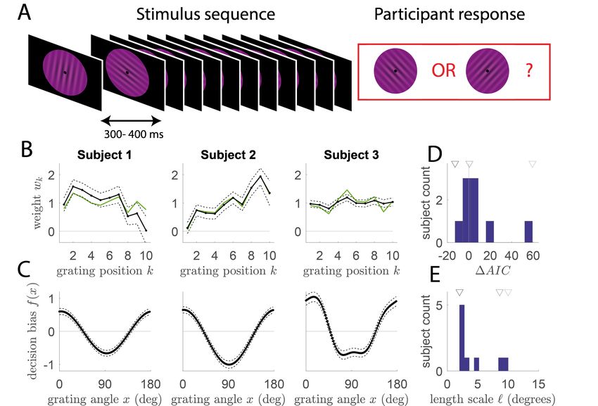
1 ( N1 k=1 wk = 1). Results are presented for three subjects in Figure 6B-6C. First, different subjects displayed
different psychophysical kernels, i.e. different profiles of grating weight wk . While subject 1 assigned more weight
to gratings presented early in the sequence (the so-called primacy effect), subject 2 assigned more weight to gratings
showed late (recency effect), and subject 3 displayed more or less equal weighting for all gratings. These patterns
obtained from the GUM matched the profiles obtained from the more traditional GLM analysis. More importantly, the
GUM analysis permitted to recover for each subject how each grating was mapped on the decision space based on its
angle, i.e. the decision mapping f (x). the mapping of subject 1 is very similar to the cosine function predicted by the
normative approach: gratings with relative angle of 0 (i.e. perfectly aligned with the reference grating) provided max-
imal bias in favor of the associated choice (rightward response), while gratings with relative angle of 90 degrees (i.e.
perpendicular to the reference grating) provided maximal bias in favor of the alternative choice (leftward response).
The mapping for subject 2 looked similar but with a vertical offset: leftward-tilted gratings provided more bias towards
left response than rightward-tilted did towards right response. Finally, mapping for subject 3 showed a much more
abrupt transition from angles biasing the decision towards the left to angles biasing towards the right response. This
is more consistent with a subject that simply categorizes the gratings as being tilted leftwards or rightwards and bases
its decision based on the counts for each category, disregarding the precise angular distance of each grating to the
references. It should be noted that GP always enforces a degree of smoothness to the recovered function, so that a step
function could not be inferred with a finite dataset.
We performed a model comparison to test, for each participant, whether the GUM provided a better account of the
behavioral data than the simpler GLM model. This analysis shows whether using a flexible mapping instead of the
fixed normative one (cosine function) improves the model. We used the Akaike Information Criterion, that corrects
the approximate marginal evidence L(q, γ) with the number of hyperparameters p (AIC = 2p − 2 log L(q, γ)). The
results were in agreement with what we observe for individual mappings (figure 6E). For subject 1, whose mapping
was very similar to the normative one, the GLM was favored. For subject 2 and 3, whose mapping differed from the
normative one, the GUM was favored. Finally, the fitted values of the hyperparameters provides an information about
the degree of smoothness of the mapping that provided the best account of the data. In particular, the values of the
length scale for the squared exponential was 4.1 ± 3.1 degrees (average ± std across participants) (figure 6D).
4 Discussion
Here we have presented a novel class of regression models, Generalized Unrestricted Models or GUMs, that allows
to capture nonlinear mapping for each regressor, as well as additional and multiplicative interactions between these
regressors. We propose a Bayesian treatment of GUMs using the framework of Gaussian Processes, that allow to define
distributions over functions with interpretable properties. Moreover, GUMs allow to perform regression for many
different data type (including binary variable, categorical, real, periodic), making it an extremely versatile analysis
method.
We have shown two different algorithms to learn GUMs from experimental data: the Laplace method and the sparse
variational approach, which scales better for larger dataset. A GUM analysis on synthetic data showed that both
methods allowed to recover mappings with low estimation error, even for small datasets. However, we strongly advise
to run parameter recovery analysis for any new GUM problem. Indeed the estimation error will largely depend on
the class of the model and the size of the dataset. For some classes of models, the identifiability may be poor. Using
multiple initial values for the estimation procedure is key to avoid finding local solutions to the estimation problem,
but may not always correct this identifiability issue.
There is a long history of using regression analyses that capture multiplicative interactions between regressors.
ANOVA is routinely used to capture these interactions for categorical regressors and continuous dependent variable.
This is equivalent to defining a GLM that includes multiplication of the regressors into the design matrix (which
is the method of choice for non-normally distributed dependent variable). For continuous regressors, previous
studies have looked at extensions of the GLM and other regression models to include bilinear or multilinear terms
[12, 21, 22, 11, 23]. As in the Laplace method, estimation techniques for such models rely on alternatively updating
the weights associated to one dimension while leaving the other weights fixed. However those regression models did
not capture multiplication of non-linearly transformed regressors (i.e. f1 (x)f2 (x)). One exception is the work of
Ahrens and colleagues who built multilinear models of neural spiking activity [22], where each neuron firing rate r(t)
is based on spatio-temporal filtering of the acoustic stimuli S(f, t) that is separable in time delay d and frequency f ,
10Figure 6: Application of GUM to analysis of human psychophysics experiment A. Behavioral paradigm. In each
trial, the participant viewed a sequence of 5-10 visual gratings with a certain orientation, interspersed with a 300-
400 ms interval. Subjects had to report at the end of the sequence whether the average orientation of the gratings
was more tilted clockwise or counter-clockwise. B. Psychophysical kernels recovered from the GUM analysis for 3
exemplar subjects. The kernel represents the weight of each grating wk as a function of its position k in the stimulus
sequence. Full black line represents the posterior mean, and dotted black lines the standard deviation, obtained using
the Laplace method. The green line represents the weights obtained from the standard GLM analysis. C. Perceptual
mapping for each subject, i.e. the decision update f (x) for each grating as a function of its orientation x relative to
the reference orientation (orientation tilted clockwise, i.e. 45 degrees). Positive (resp. negative) values indicate that
the grating biases the decision towards the ’tilted clockwise’ (resp. ’tilted counter-clockwise’) response. Perceptual
mapping were estimated from GUM model, legend as in B. D. Histogram of difference in Akaike Information Criterion
(∆AIC) between the GUM and simpler GLM, for all 9 participants. Positive values indicate that the GUM is favored,
negative that that the GLM is favored. Triangles above indicate values for the 3 subjects of panels B-C (black: subject
1; dark grey: subject 2; light grey: subject 3). E. Histogram of fitted values for hyperparameter ` that defines the
expected length scale of mapping f .
11P
i.e. E(r(t)) = f,d ff (f )ft (d)S(f, t − d). GUMs are also related to models designed to infer the latent dynamics
of underlying low-dimensional factors from simultaneous spike recordings, such as Gaussian Process Factor Analysis
(GPFA)[24] or variational Latent Gaussian Process
P (vLGP)[25].
P For example, the predictor in vLGP for spike count
for neuron n at time t is built as : ρnt = k αnk fk (t) + u βnu yn,t−u + cn , where fk is a collection of latent
processes modelled as GPs, αnk represent the weight of latent process k onto each neuron n, β represent the impact
of spike history onto neuron firing, and cn sets the baseline firing rate for neuron n. Spike count ynt is taken from
a Poisson distribution with rate exp(ρnt ). This is one possible functional shape of a GUM. One small difference in
treatment however is that weights α and β were modelled as hyperparameters rather than latent processes themselves,
in other words their solution did not model uncertainty about weight estimation.
In essence, the GUM framework expands the catalogue of models that can be estimated from data by adding multilin-
earity on top of nonlinear mappings. While it can be used as a purely predictive tool for machine learning applications,
its primary development is for inference problems, where we are interested in estimating the nature of the influence
of regressors over a certain dependent variable. The versatility of the tool, rather than simply expanding the space of
possible predictive models, is meant to be at the service of a research question where interpretability is essential. We
have provided an example here for analysis of behavioral data. In this example, the interaction between the functions
of grating position and grating angle found a natural interpretation: the weights for grating position wk represent the
impact of the grating depending on its position in the sequence, while the mapping from grating angle f (x) represent
how each grating biases the decision in favor of one choice or the other depending on its angle. We believe that many
scientific questions in neuroscience and beyond could be explored using this new tool, for example: assessing decom-
posable spectro-temporal receptive fields from neural recordings [22]; assessing complex cross-frequency coupling in
neural signals [26]; assessing how an evoked potential in EEG can be modulated parametrically by an experimental
factor [27]; etc. We are currently working on a toolbox to make this new versatile regression tool publicly available
for analysis of neural and behavioral datasets.
Acknowledgements
This research was supported by the Spanish Ministry of Economy and Competitiveness together with the European
Regional Development Fund (PSI2015-74644-JIN and RYC-2017-23231 to A.H.). The authors would like to thank
Isis Albareda for her help with the acquisition of behavioral data, V. Wyart for sharing code for the coding of the
experimental paradigm, as well as J.Pillow and M.Aoi for fruitful discussions about the GP framework.
References
[1] P. McCullagh and J. A. Nelder. Generalized Linear Models. Chapman & Hall / CRC, 1989.
[2] David JC MacKay and David JC Mac Kay. Information theory, inference and learning algorithms. Cambridge
university press, 2003.
[3] Christopher M Bishop. Pattern recognition and machine learning. Springer Science+ Business Media, 2006.
[4] Carl Edward Rasmussen and Christopher K. I. Williams. Gaussian Processes for Machine Learning (Adaptive
Computation and Machine Learning). The MIT Press, 2005.
[5] David M Blei, Alp Kucukelbir, and Jon D McAuliffe. Variational inference: A review for statisticians. Journal
of the American statistical Association, 112(518):859–877, 2017.
[6] Edward Challis and David Barber. Gaussian kullback-leibler approximate inference. The Journal of Machine
Learning Research, 14(1):2239–2286, 2013.
[7] James Hensman, Nicolo Fusi, and Neil D Lawrence. Gaussian processes for big data. arXiv preprint
arXiv:1309.6835, 2013.
[8] Michalis Titsias. Variational learning of inducing variables in sparse gaussian processes. In Artificial Intelligence
and Statistics, pages 567–574, 2009.
[9] Alexander G de G Matthews, James Hensman, Richard Turner, and Zoubin Ghahramani. On sparse variational
methods and the kullback-leibler divergence between stochastic processes. In Artificial Intelligence and Statis-
tics, pages 231–239, 2016.
[10] Matthias Bauer, Mark van der Wilk, and Carl Edward Rasmussen. Understanding probabilistic sparse gaussian
process approximations. In Advances in neural information processing systems, pages 1533–1541, 2016.
[11] Jianing V. Shi, Yangyang Xu, and Richard G. Baraniuk. Sparse Bilinear Logistic Regression. pages 1–25, 2014.
12[12] Christoforos Christoforou, Robert Haralick, Paul Sajda, and Lucas C. Parra. Second-Order Bilinear Discriminant
Analysis. Journal of Machine Learning Research, 11:665–685, 2010.
[13] Simon N. Wood. Fast stable restricted maximum likelihood and marginal likelihood estimation of semiparametric
generalized linear models. Journal of the Royal Statistical Society: Series B (Statistical Methodology), 73(1):3–
36, jan 2011.
[14] Hannes Nickisch and Matthias W. Seeger. Convex variational bayesian inference for large scale generalized
linear models. In Proceedings of the 26th Annual International Conference on Machine Learning, ICML ’09,
pages 761–768. ACM, 2009.
[15] Francis KC Hui, Chong You, Han Lin Shang, and Samuel Müller. Semiparametric regression using variational
approximations. Journal of the American Statistical Association, pages 1–24, 2019.
[16] Vincent Adam, James Hensman, and Maneesh Sahani. Scalable transformed additive signal decomposition by
non-conjugate gaussian process inference. In 2016 IEEE 26th international workshop on machine learning for
signal processing (MLSP), pages 1–6. IEEE, 2016.
[17] Vincent Adam. Structured variational inference for coupled gaussian processes. arXiv preprint
arXiv:1711.01131, 2017.
[18] R. E. Turner and M. Sahani. Two problems with variational expectation maximisation for time-series models.
In D. Barber, T. Cemgil, and S. Chiappa, editors, Bayesian Time series models, chapter 5, pages 109–130.
Cambridge University Press, 2011.
[19] Joshua I. Gold and Michael N. Shadlen. The neural basis of decision making. Annual review of neuroscience,
30:535–74, jan 2007.
[20] Valentin Wyart, Vincent de Gardelle, Jacqueline Scholl, and Christopher Summerfield. Rhythmic Fluctuations
in Evidence Accumulation during Decision Making in the Human Brain. Neuron, 76(4):847–858, nov 2012.
[21] Antoine de Falguerolles. Generalized Multiplicative Models. In COMPSTAT, pages 143–175. Physica-Verlag
HD, Heidelberg, 2012.
[22] Misha B Ahrens, J. F. Linden, and M. Sahani. Nonlinearities and Contextual Influences in Auditory Cortical
Responses Modeled with Multilinear Spectrotemporal Methods. Journal of Neuroscience, 28(8):1929–1942, feb
2008.
[23] Mads Dyrholm, Christoforos Christoforou, and Lucas C Parra. Bilinear Discriminant Component Analysis. The
Journal of Machine Learning Research, 8:1097–1111, 2007.
[24] Byron M. Yu, Jp Cunningham, Gopal Santhanam, Si Ryu, Krishna V. Shenoy, and Maneesh Sahani. Gaussian-
Process Factor Analysis for Low-Dimensional Single-Trial Analysis of Neural Population Activity. Journal of
Neurophysiology, 102(April 2009):614–635, 2009.
[25] Yuan Zhao and II Memming Park. Variational Latent Gaussian Process for Recovering Single-Trial Dynamics
from Population Spike Trains. Neural Computation, 29(5):1293–1316, may 2017.
[26] Jessica K. Nadalin, Louis Emmanuel Martinet, Ethan B. Blackwood, Meng Chen Lo, Alik S. Widge, Sydney S.
Cash, Uri T. Eden, and Mark A. Kramer. A statistical framework to assess cross-frequency coupling while
accounting for confounding analysis effects. eLife, 8, oct 2019.
[27] Benedikt V Ehinger and Olaf Dimigen. Unfold: An integrated toolbox for overlap correction, non-linear model-
ing, and regression-based EEG analysis. bioRxiv, page 360156, dec 2018.
13Appendix A Identifiability, constraints and offsets
One solution to the identifiability problem is to constrain all functions to take be null at some value and add offsets
cij . We still need to had further constraints on the offset depending on the structure of the model:
• We impose cij = 1 for j > 1. This avoids equivalent models by scaling all fk(i1l) and ci1 by λ, and all fk(ijl)
and cij by 1/λ).
• If there is any fixed function in factor j, i.e if there is one fk(ijl) = hk(ijl) , then the offset is not needed
because setting the value of this function removes the scaling equivalency. Therefore we set cij = 0, and
remove all constraints on functions in factor j.
• we also impose ci1 = 0 if Di = 1. If there is no interaction terms for block i, as in a standard GAM, then we
need to remove the equivalence between parameters c1i and c0 .
P the constraints above, our model will be identifiable, unless there is a null factor, i.e. unless there is (i, j)
Provided
where l fk(ijl) (x) = 0 for all x ∈ X . Note that it is also possible, when offset cij is not constrained, to absorbe it into
one of the functions in the factor (and remove the constraint on that function). For example instead of f1 (x)+f2 (x)+c
with a constraint on f1 and f2 , we can use equivalently f1 (x) + f2 (x) with a constraint on f2 only.
The form of the constraint on each f does not necessarily have to be that f (x0 ) = 0 for a given x0 . A different
constraint may be used to facilitate the interpretations of the results. For example, in the experimental analysis of
Figure 6, we chose a constraint that the average of the weights wk be 1. In general, ee will use linear constraints on
function evaluations pTk fk = lk . By identifying an orthonormal basis Pk for the subspace of RV that is orthogonal
to pk , we project fk onto this subspace and obtain free parameters θ̃ k = Pk fk ∼ N (Pk µk , Pk Kk PTk ), such that
fk = pk lk + PTk θ̃ k . If there is no constraint on a set of weights we simply have Pk = I and lk = 0. In practice we
will use four types of constraint:
1. first-zero constraint, i.e. fk (x0 ) = 0, is the default constraint that the function must be null at some defined
value x0 . The projection matrix Pk is simply the identity matrix deprived of the corresponding line.
P
2. mean-zero constraint, i.e. n fk (n) = 0. This corresponds to lk = 0 and corresponding projection matrix
Pk (m, n) = √ 1 if m ≥ n, Pk (m, m + 1) = − √ m and Pk (m, n) = 0 if m < n. This constraint
m(m+1) m(m+1)
P
is useful in the GAM context, i.e. when the activations are taken as the sums of GPs ρ(x) = k fk (xk ). In
GUMs, we will generally impose mean-zero constraint for all but one functions inserted in one-dimensional
components.
P
3. mean-one constraint, i.e. n fk (n) = lk = 1 (the projection matrix is same as for mean-zero constraint).
This is equivalent to mean-zero constraint and absorbing offset c = 1.
P
4. sum-one constraint, i.e. n fk (n) = Vk , is an alternative to mean-one constraint.
Appendix B Laplace approximation for GUM
B.1 Conversion to GMM with Gaussian prior
The parameters to infer are θ = {f1..K , c}, where fk = fk (xk ) and xk the vector of vk unique values taken by xs(k)
in the dataset. fk have MVN prior N (µk , Kk ) and each offset parameter has normal prior N (0, σ 2 ), so θ has MVN
prior with mean (µ1 , ..µK , 0) and a block-diagonal covariance matrix. Instead of fully flexible functions fk , we can
also impose linearity, i.e. fk (x) = wkT xsk . In this case, we define an isometric MVN prior on the weights (akin to
L2-regularization), i.e. fk = wk and fk ∼ N (0, σk2 I).
We can write fk (x(n) ) = Φkn · θ where Φkn is an indicator vector of length vk whose value 1 indicates the position
of the corresponding parameter in the parameter set. If function fk decomposes as the product of a fixed function hk
and function to be estimated f˜k , then parameters are fk = f˜k (x) and the values of Φkn are changed to hk (x(n) ). In
the case of linear mapping, we have Φk = (xs(k) ) (i.e. the classical design matrix of a GLM). Finally a fixed function
fk = hk has no parameter.
P
The values taken by factor Fij (x) = l fk(ijl) (x) in the dataset is Fij = Fij (X) = Φij θ ij + Cij , where θ ij is the
subset of θ that parametrises factor Fij , the design matrix Φij for factor Fij is built by concatenating design matrices
Φk(ijl) for individual functions, and including also the term for dependence in offset cij if it is a free parameter. Cij
sums all fixed values, i.e. hk for fixed functions fk in the factor, and cij if its value is fixed.
14Now we see that the equation of a GUM (equation 1) can be replaced with a generalized multilinear model [11, 22]
with C blocks and Gaussian priors for the weights:
Di
C Y
X
ρ= (Φij θ Tij + Cij ) (6)
i=1 j=1
B.2 Maximum A Posteriori weights
To identify the Maximum A Posteriori solution, we use the general solution for generalized multilinear models which
is to optimise over set of parameters in one factor while keeping others factors in the block constant, pass on the next
factor and iterate until convergence ([22]). At each iteration, we optimise weights over factor ji? for each block i. The
optimization is possible as long as the parameters θ ij in the factors are not also present in the factors that are fixed,
i.e. if there are no calls to the same function in the different factors of the same block (the method cannot be applied
to model ρ(x) = f1 (x)(f1 (x) + f2 (x)). However it is perfectly possible to have different calls to the same function
in different blocks, for example defining ρ(x) = f1 (x1 )f2 (x2 ) + f1 (x3 )f4 (x4 ).
The generative model transforms to :
P
ρ = (Φ ? θ ? + Ci,j? )
Pi (i,¬ji ) Ti,ji i
?
= i Φ (i,¬ji ) i,ji? θ̃ i,ji? + C , where
? P (7)
C? T
P
= i (Ci,ji + pi,ji Φ(i,¬ji ) pi,j? )
? ? ?
i
T
where the new covariates are obtained by collapsing over fixed factors j 6= ji? : Φ(i,¬ji? ) =
Q
j6=ji? (Φij θ ij + Cij ). We
see that the predictor is linear with respect to the set of weights θ̃ corresponding to all θ̃ i,ji? in all blocks i. We thus
obtain the generative equation from a GLM with MVN prior:
?T
g(E(y (n) ))) = ρ = Φ̃? θ̃ + C? (8)
h i P(1,j1? )
where Φ̃? = Φ? P?T , Φ?n = Φ(1,¬j1? ) . . . Φ(C,¬jC? ) and P? = ...
P(C,jC? )
? ?
We update the set of weights θ̃ with a single Newton-Raphson update. Prior mean for θ̃ is MVN, with means µ?
?
and covariance K? extracted from the µ and K. The log-posterior over θ̃ can be expressed as:
? ? ?
(
log p(θ̃ |y) = log(y|θ̃ ) + log p(θ̃ ) + const
PN ? ? (9)
= 1
s n=1 (ηn y
(n)
− B(ηn )) − 21 ((θ̃ −µ̃? ))T (K? )−1 (θ̃ −µ̃? ) + const
where ηn and s are respectively the canonical and dispersion parameter of the exponential family distribution for yn ,
and B(ηn ) is such that dB
dη = E(y
(n)
) = g −1 (ρn ). In the following we assume that g is the canonical link function
(similar updates can be found in the general case).
?
Since the gradient of ρ(n) w.r.t weights θ̃ is Φ?n P? , the gradient and Hessian of the log-posterior gives:
? ?
( PN
∇ log p(θ̃ |y) = 1s n=1 Φ̃?T
n (y
(n)
− g −1 (ρn )) − (K? )−1 (θ̃ −µ̃? )
? N ? −1
(10)
= − 1s n=1 Φ̃?T ?
P
∇∇ log p(θ̃ |y) n Rnn Φ̃n − (K )
R is a diagonal matrix such that Rnn = (g −1 )0 ρ(n) = 1
g 0 (g −1 (ρ(n) ))
.
The Newton-Raphson update gives:
? ? ? ?
θ̃ new = θ̃ − (∇∇ log p(θ̃ |y))−1 ∇ log p(θ̃ |y)
? ?
= θ̃ + (K? Φ̃?T RΦ̃? + sI)−1 (K? Φ̃?T (y−g −1 (ρ)) − s(θ̃ −µ̃? ))
= H −1 B with (11)
H = K? Φ̃?T RΦ̃? + sI
B = K? Φ̃?T (Rρ̃ + y − g −1 (ρ)) + sµ̃?
15?
We have defined ρ̃ = Φ̃? P? θ̃ = ρ − C? . From equation (11) we obtain the new values for all weights θ (i,ji? ) . The
algorithm loops by selecting at each iteration a new set of factors ji? and then applying equations (7,8, 11) to update
the values of θ (i,ji? ) .
If there are several set of unconstrained weights in the same block, convergence may take many iterations as the
scaling of the weights are only constrained by the different priors. In such cases, it is convenient to re-scale these set
of weights after each iteration to speed up convergence time:
1
Q free
( j0 αij 0 ) ) 2Di
θ new
ij = √ θ ij , with αij = (θ ij − Pij )T (Kij )−1 (θ ij − vKij )T (12)
αij
The product is taken over all free constraint dimensions in the component (Difree is the number of such dimensions).
B.3 Posterior covariance
In the Laplace approximation, the posterior mean is provided by the MAP weights while the posterior covariance for
weights is approximated from the full Hessian of the log-posterior. Hessian for free weights in the same set (same
component, same dimension) are provided by equation 11. For free weights in different sets θ ij and θ (i0 j 0 ) , we have:
∇θ̃ij ∇θ̃i0 j0 log p(θ̃|y) = (Φ(i,¬j) )T RΦ(i0 ,¬j 0 ) (13)
Once we have identified the approximate posterior covariance for free parameters Σ̃ = −(∇θ̃ ∇θ̃ log p(θ̃|y))−1 , we
recover the posterior for parameters θ which is Σ = PT Σ̃P (matrix P is is block diagonal formed with all Pk for all
components and dimensions).
The Laplace approximation can be used to generate predictions for fk (x0 ) at values of x0 not included in the training
set ([4]):
fk (x0 ) = N (m0 , (v 0 )2 ) , where
m0 = Kk (x0 , xk )(Kk )−1 fkMAP (14)
0 2
(v ) = Kk (x0 , x0 ) − Kk (x0 , xk )T (Σk )−1 Kk (x0 , xk )
The Laplace approximation can also be used to approximate the log-marginal evidence p(y) ([4]):
1 MAP MAP MAP 1 1
log p(y|X) ≈ − (θ̃ − µ̃)T K̃ −1 (θ̃ − µ̃) + log p(y|X, θ̃ ) − log |I + K̃W | (15)
2 2 2
B.4 Hyperparameter fitting
B.4.1 Maximising cross-validated score
MAP MAP
Here, we first find MAP values θ̃ from a training set (x, y) and compute a fitting score for θ̃ =
arg max p(θ̃|x, y, γ) on a cross-validation set (X 0 , y 0 ). We wish to find hyperparamaters γ that maximises the cross-
validated score S(θ̃; X 0 , y 0 ). Here we will use the log-likelihood as the score, i.e. S(θ̃; X 0 , y 0 ) = log(y 0 |X 0 , θ̃). The
gradient of the score w.r.t to hyperparameters can be computed using the chain rule:
( MAP MAP MAP
∇γ S(θ̃ ; X 0 , y 0 ) = ∇γ θ̃ · ∇θ̃ S(θ̃ ; X 0 , y0 )
MAP Pn0 (16)
1
= s ∇γ θ̃ · P k=1 (yk0 − g −1 (ak0 )∇U ak0
From equation 7, we can see that the gradient of ak0 is obtaining by concatenating pseudo-design matrices
(1,¬1) (C,¬D ) MAP
(Φ.k0 , .., Φ.k0 C ) . From the definition of the MAP weights θ̃ , the Jacobian with respect to hyperparam-
eters is: MAP MAP
∇γ θ̃
= −H −1 (∇γ ∇θ̃ log p(θ̃ |X, y, γ))
−1 MAP
= −H P (∇ ∇
γ U log N ( θ̃ ; 0, K(γ))) (17)
−1 −1 −1 MAP
= −H P K ∇γ KK θ̃
16You can also read


