Nonstationary weather and water extremes: a review of methods for their detection, attribution, and management - HESS
←
→
Page content transcription
If your browser does not render page correctly, please read the page content below
Hydrol. Earth Syst. Sci., 25, 3897–3935, 2021
https://doi.org/10.5194/hess-25-3897-2021
© Author(s) 2021. This work is distributed under
the Creative Commons Attribution 4.0 License.

Nonstationary weather and water extremes: a review of methods
for their detection, attribution, and management
Louise J. Slater1 , Bailey Anderson1 , Marcus Buechel1 , Simon Dadson1,5 , Shasha Han1 , Shaun Harrigan2 ,
Timo Kelder3 , Katie Kowal1 , Thomas Lees1 , Tom Matthews3 , Conor Murphy4 , and Robert L. Wilby3
1 School  of Geography and the Environment, University of Oxford, Oxford OX1 3QY, UK
2 Forecast Department, European Centre for Medium-Range Weather Forecasts (ECMWF), Reading, UK
3 Geography and Environment, Loughborough University, Loughborough, UK
4 Irish Climate Analysis and Research UnitS (ICARUS), Department of Geography,

Maynooth University, Maynooth, Co. Kildare, Ireland
5 U.K. Centre for Ecology and Hydrology, Maclean Building, Crowmarsh Gifford, Wallingford OX10 8BB, UK

Correspondence: Louise J. Slater (louise.slater@ouce.ox.ac.uk)

Received: 7 November 2020 – Discussion started: 14 November 2020
Revised: 15 April 2021 – Accepted: 19 May 2021 – Published: 7 July 2021

Abstract. Hydroclimatic extremes such as intense rainfall,        not exhibit any shift in mean, variance (Fig. 1b), or shape.
floods, droughts, heatwaves, and wind or storms have devas-       For hydroclimatic extremes, this implies that the distribution
tating effects each year. One of the key challenges for society   of extreme precipitation, temperature, streamflow, or wind
is understanding how these extremes are evolving and likely       should merely fluctuate within a stationary envelope of vari-
to unfold beyond their historical distributions under the in-     ability. The assumption of stationarity has long served as the
fluence of multiple drivers such as changes in climate, land      basis for the statistical analysis of hazards and the design of
cover, and other human factors. Methods for analysing hy-         engineering structures, by defining the magnitude of events
droclimatic extremes have advanced considerably in recent         with a given frequency of occurrence, such as the stationary
decades. Here we provide a review of the drivers, metrics,        100-year design flood (e.g. Salas et al., 2018).
and methods for the detection, attribution, management, and          In reality, the global water cycle manifests many artificial
projection of nonstationary hydroclimatic extremes. We dis-       patterns and trends induced by human activities such as cli-
cuss issues and uncertainty associated with these approaches      mate change, land cover change (e.g. Blum et al., 2020), wa-
(e.g. arising from insufficient record length, spurious non-      ter abstraction or augmentation, river regulation, and even
stationarities, or incomplete representation of nonstationary     geopolitical uncertainty (e.g. Wine, 2019) at local, regional,
sources in modelling frameworks), examine empirical and           and global scales. Trends and step changes in the magnitude,
simulation-based frameworks for analysis of nonstationary         frequency, duration, volume, or areal extent of hydroclimatic
extremes, and identify gaps for future research.                  extremes, such as intense rainfall (e.g. Sun et al., 2020a; Wes-
                                                                  tra et al., 2013; Donat et al., 2016), floods (e.g. Berghuijs
                                                                  et al., 2019a; Do et al., 2017; Archfield et al., 2016), droughts
                                                                  (e.g. Andreadis and Lettenmaier, 2006; Spinoni et al., 2017),
1   Introduction: nonstationary hydroclimatic extremes            and heatwaves or heat stress (e.g. Oliver et al., 2018; Lorenz
                                                                  et al., 2019; Ouarda and Charron, 2018), have been widely
Are hydroclimatic extremes stationary or nonstationary?           detected and have led to proclamations about the “death” of
This question has generated much debate because of the ram-       stationarity in water management (Milly et al., 2008). In con-
ifications for hazard management in a changing world. At the      trast, trends in strong winds or storms are less certain, and
simplest level, a stationary process is one in which the sta-     the influence of anthropogenic climate change is difficult to
tistical properties of the distribution and correlation do not    attribute (Shaw et al., 2016; Elsner et al., 2008; Martínez-
shift over time. Thus, a stationary time series (Fig. 1a) would

Published by Copernicus Publications on behalf of the European Geosciences Union.
3898                                                     L. J. Slater et al.: Nonstationary weather and water extremes: a review

Figure 1. What is nonstationarity? Examples of (a) a stationary time series with constant mean and variance and (b) three nonstationary time
series in the form of a shift in mean (trend and step change) and a shift in variance. Solid and dashed black lines represent the mean and the
variance of the time series, respectively.

Alvarado et al., 2018; Wohland et al., 2019). Disentangling              plication of nonstationary analysis. A growing body of lit-
natural and anthropogenic drivers of nonstationarity is prob-            erature has shown that inappropriately applying nonstation-
lematic as the two can be interlinked, and even seemingly                ary models to short time series may have the undesired ef-
“natural” drivers such as climate modes may shift under the              fect of increasing uncertainty; in cases where model struc-
effects of anthropogenic climate change (e.g. Maher et al.,              ture and/or underlying physical drivers are uncertain, station-
2018). Although the drivers of abrupt nonstationarities (step            ary models may be the preferred option for design and man-
changes) may be apparent (e.g. water abstraction, reservoir              agement of extremes (Serinaldi and Kilsby, 2015). Nonsta-
filling, and operations), drivers of more incremental non-               tionarity should not be presumed to occur everywhere sim-
stationarities (trend or variance; e.g. climate variability and          ply because of climate change (Lins, 2012); nonstationary
change and land cover change) may be harder to attribute                 approaches have value primarily when there are good rea-
and/or obfuscated by other confounding factors.                          sons to suspect physically plausible and predictable drivers
    Deciding whether to employ nonstationary methods for                 of change.
the purpose of managing extremes is thus a key challenge                    Over the last 2 decades, hundreds of papers have addressed
facing weather and water scientists and practitioners today              the detection, attribution, prediction, and projection of non-
(e.g. Faulkner and Sharkey, 2020), as it is unclear how to               stationarity in precipitation, floods, drought, heat stress, tem-
represent increased uncertainty arising from climate change              perature, extreme winds, and storms. However, a compre-
(e.g. Wasko et al., 2021). Detecting the presence, and at-               hensive introductory overview of these methods across hy-
tributing the source of nonstationarity in hydroclimatic ex-             droclimatic extremes, including an overarching discussion of
tremes, is, however, vital for understanding and managing                the key challenges that can arise, has not been published to
water resources in a changing world. Nonstationarity may                 date. This paper is the first to review the entire nonstation-
have dramatic impacts for infrastructure (François et al.,               ary management process, from identifying metrics to anal-
2019), property, and society over a range of overlapping                 ysis through to management. This paper offers a synthesis
timescales. There are many different drivers that may alter              of methods for quantifying, attributing, and managing non-
extremes simultaneously over both the short term (such as                stationarity over multiple spatial and temporal scales, along
human management impacts) and medium to long term (such                  with their limitations. The structure follows the logical order
as land cover and climate change impacts) (e.g. Warner,                  of steps employed in a detection, attribution, and manage-
1987; Rust et al., 2019). Short-term trends are widely present           ment framework (Fig. 2). Challenges are presented for each
in variables like streamflow, which exhibit long memory                  step throughout the paper.
(time dependence) and periodicities. However, such trends                   Section 2 describes the most widely used indices for diag-
are not necessarily indicative of nonstationarity (e.g. Kout-            nosing the symptoms of nonstationarity via changes in mag-
soyiannis, 2006; Koutsoyiannis and Montanari, 2015). “Non-               nitude, frequency, and timing. Section 3 identifies essential
sense correlations” can be found between time-varying vari-              data prerequisites for detecting nonstationarity, such as ho-
ables without any physical significance (Yule, 1926), and ap-            mogeneity analysis. Section 4 discusses the techniques used
parent trends or oscillations may be found in time series due            to detect nonstationarity, including regression-based methods
to random causes (Slutzky, 1937). In fact, random fluctua-               for gradual change, pooled approaches for analysis of rare
tions or deviations from the mean are to be expected in sta-             extremes, step change analysis for abrupt change, and other
tionary time series (e.g. Wunsch, 1999), especially those with           methods for discerning changing seasonality. Section 5 intro-
a long memory. Multi-decadal (e.g. 30 year) shifts may sim-              duces the key drivers of nonstationarity of hydroclimatic ex-
ply be temporary excursions in longer (e.g. 100 year) records,           tremes. Section 6 reviews approaches for attribution of non-
or a function of the start and end dates chosen for the trend            stationary extremes, including both observation- and model-
analysis (Harrigan et al., 2018), and may not warrant the ap-            based approaches, and issues with attribution and engineer-

Hydrol. Earth Syst. Sci., 25, 3897–3935, 2021                                               https://doi.org/10.5194/hess-25-3897-2021
L. J. Slater et al.: Nonstationary weather and water extremes: a review                                                             3899

Figure 2. Workflow for the detection, attribution, and management of nonstationary hydroclimatic extremes. Bullet points indicate examples
discussed in the paper (Sects. 2–7).

ing design under nonstationarity. Finally, Sect. 7 discusses           precipitation accumulation for a given duration (1, 3, or 6 h
approaches for managing nonstationarity via engineering de-            and 1 or 5 d, termed Rx1day or Rx5day, respectively) within
sign and model projections, including key limitations. The             a given month, season, or year (e.g. Champion et al., 2019;
overall aim of the paper is to highlight the most significant          Sun et al., 2020a). This includes the percentage of rain that
issues and considerations when detecting, attributing, pre-            fell in the monthly maximum 1 h precipitation (or some
dicting, and projecting nonstationarity in hydroclimatic ex-           other period), the 90th, 95th, or 99th percentile precipitation
tremes.                                                                amount (over 1, 3, or 6 h) during a month or year – or, specif-
                                                                       ically, on wet days (Moberg and Jones, 2005) – or even the
                                                                       total precipitation accumulated from hours exceeding speci-
2     Symptoms of nonstationarity                                      fied percentiles over a month or year (e.g. Donat et al., 2013).
                                                                       For instance, at the global scale, analysis of the Rx1day and
Nonstationarities in hydroclimatic extremes may be ex-
                                                                       Rx5day precipitation accumulations found that extreme pre-
pressed through a significant shift in the mean, variance, or
                                                                       cipitation has increased at about two-thirds of stations – a sig-
shape of a given time series (Fig. 1). Such departures are gen-
                                                                       nificantly greater proportion than can be expected by chance
erally diagnosed by symptoms such as a change in the mag-
                                                                       (Sun et al., 2020a). An important concept is the probable
nitude (events becoming more or less extreme), frequency
                                                                       maximum precipitation (PMP), i.e. the greatest depth of pre-
(events occurring more or less often than before), and timing
                                                                       cipitation that is possible in a given place and time and for
(events occurring earlier or later in the year) of seasonal or
                                                                       a given storm duration. For a complete state-of-the-art re-
annual extremes. There are many different ways of describ-
                                                                       view on the PMP concept, see Salas et al. (2020). PMP can
ing the symptoms of nonstationarity – each is discussed in
                                                                       be computed via hydrometeorological, statistical, grid-based,
turn below, and examples are provided in Table 1.
                                                                       and site-specific approaches, using both stationary and non-
2.1    Magnitude                                                       stationary methods (e.g. Lee and Singh, 2020). PMP is ex-
                                                                       pected to increase in many regions in future decades due
Significant changes in the magnitude of extremes are rel-              to increases in atmospheric moisture content and moisture
evant to society, engineers, decision makers, and insurers             transport into storms (Kunkel et al., 2013).
alike. The magnitude or intensity of an event is generally de-            Percentiles of daily streamflow distribution are commonly
scribed by estimating the percentiles of a distribution over a         used for floods (Fig. 3b). For example, the Q90 (the 90th
given period. Examples may include the peak rainfall, peak             percentile of the distribution, i.e. the flow that is exceeded
streamflow, peak intensity of a drought, maximum/minimum               10 % of the time, confusingly referred to as “Q90 ” in North
temperature, or peak wind speed within a given day, month,             America and “Q10 ” in Great Britain and Ireland), Q95 , Q99
season, or a year (Fig. 3). Significant changes are detected           (flow that is exceeded 3.65 d per year, on average), Q99.9
by evaluating alterations in these percentiles over time (e.g.         (0.37 d per year), or AMAX (the annual maximum stream-
a time series of annual maximum daily streamflow). More                flow). When considering more extreme events than AMAX,
generally, magnitudes can also be described via metrics char-          hydroclimatic extremes are commonly expressed as 1 in 20-
acterizing the intensity or flashiness of an event, such as its        , 1 in 50-, or 1 in 100-year events (e.g. Milly et al., 2002;
spatial extent, duration, or time to peak (Fig. 3).                    Slater et al., 2021). Hydrograph analyses may also be used to
   The magnitude or intensity of precipitation (in millime-            extract metrics such as flood volume and duration (Fig. 3b).
tres; Fig. 3a) can be assessed using various metrics. Many             Other indicators describe the flashiness of an event, such as
of these are part of the ETCCDI indices that were proposed             the time to peak, which is defined as the total number of
in 2002 by the expert team on climate change detection and             hours starting from the sharp rise of the hydrograph until
indices (ETCCDIs; see, e.g., Frich et al., 2002; Zhang et al.,         the peak discharge. The spatial extent of a flood event can
2011). Precipitation metrics include the maximum depth of              be described using metrics such as the number of catchments

https://doi.org/10.5194/hess-25-3897-2021                                            Hydrol. Earth Syst. Sci., 25, 3897–3935, 2021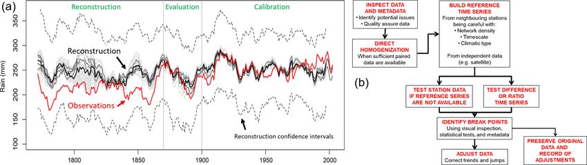
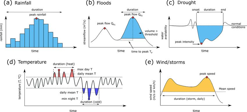
3900                                                 L. J. Slater et al.: Nonstationary weather and water extremes: a review

Figure 3. Metrics employed for evaluating five types of hydroclimatic extremes. (a) Precipitation hyetograph. (b) Flood hydrograph.
(c) Drought. (d) Temperature. (e) Wind (storms). All these variables can be described using indicators of event duration and magnitude
(peak intensity).

flooding simultaneously (Uhlemann et al., 2010) or the flood         locally, using composite indicators including precipitation
synchrony scale (FSS), which evaluates the largest radius            and temperature. Various metrics exist to measure drought
around a stream gauge where more than half of the surround-          stress, and they either reflect deficits in precipitation or com-
ing stream gauges also record flooding within the same week          bined metrics of precipitation, temperature, and evapora-
(Berghuijs et al., 2019a). Studies are increasingly evaluating       tion. The World Meteorological Organization (WMO) rec-
the spatial dependence of flooding across multiple basins by         ommends the use of the Standardized Precipitation Index
considering meteorological, temporal, and land surface pro-          (SPI), which reflects standard deviations from normal rain-
cesses leading to simultaneous flooding across varying spa-          fall (WMO, 2016; McKee et al., 1993). Other well-known
tial scales (e.g. Brunner et al., 2020; Kemter et al., 2020;         indices that rely on monthly precipitation include the Palmer
Wilby and Quinn, 2013).                                              drought severity index (PDSI; Palmer, 1965), deciles (Gibbs
   Droughts (Fig. 3c) differ from other extreme weather be-          and Maher, 1967), and the rainfall anomaly index and its
cause they develop more slowly and last longer; they are             modified version (RAI and mRAI, respectively; e.g. Hänsel
broadly defined as “a sustained period of below-normal water         et al., 2016). Some metrics combine variables; for instance,
availability” (Tallaksen and Van Lanen, 2004) and are some-          PDSI is computed using precipitation and potential evapo-
times referred to as a “creeping phenomenon” (Mishra and             transpiration. The Standardized Precipitation Evapotranspi-
Singh, 2010; Wilhite, 2016). These characteristics make it           ration Index (SPEI) can be interpreted similarly to SPI but
more difficult to assess nonstationarity as there are fewer          reflects both evaporative demand and precipitation inputs to a
events to compare over time; plus, drought onset and ter-            system (Vicente-Serrano et al., 2010). The spatial character-
mination are challenging to pinpoint (Parry et al., 2016).           istics of drought have also become increasingly relevant, as
Not all droughts are defined by aridity, and rainfall deficit        more studies examine their areal extent over time, using met-
alone does not imply a drought (Van Loon, 2015). Instead,            rics like spatial patterns of drought intensity mapped across
a combination of factors in the hydrological cycle inter-            livelihood zones over time (e.g. Leelaruban and Padmanab-
act to yield below-normal conditions (Fig. 3c). Drought has          han, 2017; Mekonen et al., 2020).
been typically classified as being meteorological (precipi-             For temperature extremes (Fig. 3d), studies may monitor
tation deficit), hydrological (surface and subsurface water          the hottest/coldest day, the warmest/coolest night, or the ex-
deficit relative to local water uses), agricultural (declining       treme temperature range (TXx–TNn; degrees Celsius) over
soil moisture and crop failure), or socioeconomic (failure of        a given period, i.e. a month, season, or year (e.g. Donat
water resources system to meet demand) (Van Loon, 2015).             et al., 2013; Papalexiou et al., 2018). Globally, the highest
Since the definition of normal conditions depends on spatial         temperature of the year, for example, increased by 0.19 ◦ C
and temporal scales, drought anomalies are typically defined         per decade during 1966–2015 but accelerated to 0.25 ◦ C per

Hydrol. Earth Syst. Sci., 25, 3897–3935, 2021                                          https://doi.org/10.5194/hess-25-3897-2021
L. J. Slater et al.: Nonstationary weather and water extremes: a review                                                     3901

decade during 1986–2015, displaying a faster increase than        son/year. In reality, the magnitude and frequency of extremes
the mean annual temperature (Fig. 4b, Papalexiou et al.,          are closely related, such that when magnitudes increase, one
2018). Percentiles of the distribution are also commonly as-      can also typically expect to find more peaks over a given
sessed (Zhang et al., 2005; Kjellström et al., 2007), while       threshold (see Fig. 4). Frequency-based metrics, however,
some authors work with combined temperature–humidity              generally enable better detection of changes in extremes
metrics (Matthews et al., 2017; Raymond et al., 2020b; Knut-      than in magnitude-based metrics (e.g. Mallakpour and Vil-
son and Ploshay, 2016) which offer a more complete measure        larini, 2015) because they often reflect a larger sample of
of atmospheric heat content (Pielke et al., 2004; Peterson        data and are less prone to measurement errors. For exam-
et al., 2011; Matthews, 2020) and may, therefore, be more         ple, while block maxima approaches often include just one
closely aligned with levels of thermal stress felt by humans      value per year/season, POT approaches count the total num-
(Mora et al., 2017; Matthews, 2018). Other approaches in-         ber of exceedances above a threshold. This fact is exploited
clude an emphasis on duration by focussing on heatwaves,          by those using documentary evidence to evaluate flood fre-
defined as periods of consecutive days when heat is higher        quency (Macdonald et al., 2006). The thresholds for detec-
than normal (Perkins and Alexander, 2013). This very broad        tion of changes in frequency should be set high enough to
categorization has seen a plethora of thresholds (both ab-        describe a meaningful extreme event yet low enough to com-
solute value and percentile based) and metrics (tempera-          pile an adequate sample size.
ture and combined temperature–humidity indices) applied to            For precipitation, independent events must be first iden-
heatwave studies, with the choice shaped by interests in po-      tified for POT analysis. Various approaches exist for the
tential impacts (Xu et al., 2016).                                identification of events, such as the fitting of Poisson mod-
   Changes in the magnitude of extreme wind events (Fig. 3e)      els (Restrepo-Posada and Eagleson, 1982). Multiple methods
may also be tracked using wind speed percentiles such as          also exist for the selection of the most appropriate thresh-
the 90th, 95th, 98th, and 99th seasonal or annual percentiles     old (Caeiro and Gomes, 2016). Thresholds are generally cho-
(e.g. Donat et al., 2011; Young and Ribal, 2019; Wang et al.,     sen based on the local precipitation distribution such as the
2009). For instance, the 90th percentile of 10 m wind speed       95th, 98th, 99th, or 99.5th percentile of rain over a 1, 6,
from ERA-Interim reanalysis data exhibits increasing wind         12, or 24 h period (e.g. Wi et al., 2016). Percentile or fixed
speeds over the tropical oceans and large parts of South          thresholds (such as the 10 or 20 mm daily total, denoted
America but decreasing trends over eastern Europe and             as R10mm or R20mm, respectively) are then used to count
northwestern Asia (Fig. 4e, Torralba et al., 2017), although      monthly/annual days with heavy precipitation exceeding or
trends vary widely across reanalysis products (Torralba et al.,   equalling these values. Alternatively, a mean residual life plot
2017; Wohland et al., 2019). Wind intensity (in metres per        (an exploratory graphical approach) can be used to select
second) may be explicitly measured over 2 min sustained pe-       a suitably high threshold (e.g. Coles, 2001). These thresh-
riods, or 3 s gust periods (Pryor et al., 2014). Wind events      olds can be calculated for individual years or using the en-
may also be inferred from gradients in sea level pressure         tire multi-year record. For an overview of threshold selec-
fields (Jones et al., 2016; Matthews et al., 2016b). Winds as-    tion methods, see Anagnostopoulou and Tolika (2012). At
sociated with Western Hemisphere tropical cyclones are de-        the global scale, increases in the frequency of extreme pre-
scribed using storm scales such as the Saffir–Simpson hur-        cipitation have been more pronounced than changes in mag-
ricane wind scale (SSHWS; e.g Elsner et al., 2008; Karl           nitude (Fig. 4a, b, Papalexiou and Montanari, 2019). An al-
et al., 2008). This classifies wind intensity into the follow-    ternative approach for estimating the probability of intense
ing five storm categories: one (119–153 km/h), two (154–          rainfall events is the changing likelihood of an historical pre-
177 km/h), three (178–208 km/h), four (209–251 km/h), and         cipitation analogue (Matthews et al., 2016a).
five (>252 km/h). Cyclones and typhoon magnitudes are                 The frequency of temperature extremes is assessed using
equally described using metrics such as the seasonal mean         metrics such as the percentage of time when the daily mini-
lifetime peak intensity, intensification rate, and intensifica-   mum or maximum temperature is below or above a given per-
tion duration (Mei et al., 2015).                                 centile, such as the total annual count of ice/frost days (ID or
                                                                  FD, respectively), where the daily minimum temperature is
2.2   Frequency                                                   below 0 ◦ C (e.g. Donat et al., 2013). Mwagona et al. (2018)
                                                                  observed changes in cold/warm night frequency at 116 sta-
A second broad category of nonstationarity symptoms is            tions in northeastern China. They report a decrease in cold
the frequency of events. Many metrics are used to describe        night frequency during winter and spring, while warm night
changes in the frequency of hydroclimatic extremes, such          frequency increased primarily in summer. Similar metrics
as annual exceedance probabilities and counts of occur-           are used to describe changes in the frequency of heatwaves
rences above or below thresholds. Examples of such peak           (Perkins-Kirkpatrick and Lewis, 2020) or growing season
over threshold (POT) approaches may include the number            days, such as the number of days with plant heat stress (with
of days or hours above/beneath a temperature threshold, or        maximum temperature exceeding 35 ◦ C; e.g. Rivington et al.,
the number of flood or drought events, within a given sea-        2013). Alternatively, the accumulated frost (sum of degree

https://doi.org/10.5194/hess-25-3897-2021                                      Hydrol. Earth Syst. Sci., 25, 3897–3935, 2021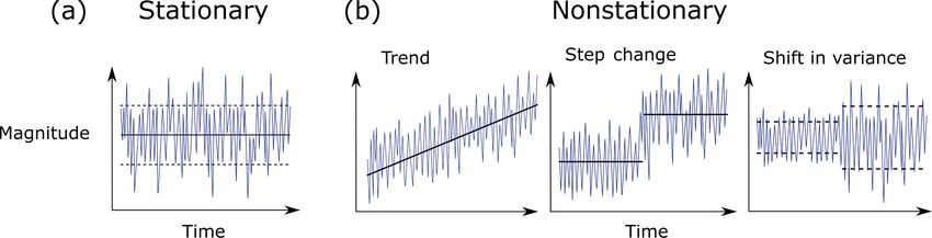
3902                                                    L. J. Slater et al.: Nonstationary weather and water extremes: a review

Table 1. Examples of indicators employed for the detection of nonstationarity in weather and water extremes. More detailed tables of metrics
can be found in Donat et al. (2013) for temperature and precipitation or Ekström et al. (2018) for a detailed list of hydroclimatic metrics.

  Type          Common indicators              Example application                                Example reference
  Magnitude     Percentiles/quantiles          – 90th percentile of rain on wet days              Moberg and Jones (2005)
                                               – 1 in 20/50/100-year flood event                  Slater et al. (2021)
                Maxima/minima                  – Annual maximum wet bulb temperature              Raymond et al. (2020b)
                                               – Temp. of hottest/coldest day/night               Donat et al. (2013)
                                               – Annual max. daily streamflow (Q100 )             Do et al. (2017)
                                               – Annual max. of 1 d rain (Rx1day)                 Scherrer et al. (2016)
                Extent                         – Flood synchrony scale (FSS)                      Berghuijs et al. (2019a)
                                               – Storm radius with winds > 34/50/64 knots         Zhai and Jiang (2014)
                Duration                       – Consecutive drought months                       Vicente-Serrano et al. (2021)
                                               with SPI < value
  Frequency     Occurrences                    – Number of heatwave days                          Perkins-Kirkpatrick and Lewis (2020)
                                               – Number of flood peaks (POT)                      Prosdocimi et al. (2015)
                                               – Number of tropical cyclones (TCs)                Walsh et al. (2016)
                Probability                    – Heavy rain annual exceedance prob. (AEP)         Corella et al. (2016)
                                               – Likelihood of historical precip. analogue        Matthews et al. (2016a)
                                               – Climatic drought probability ratio (PR)          Ma et al. (2017)
  Timing        Date                           – Centre-volume date                               Dudley et al. (2017)
                                               – Ordinal day of AMAX streamflow                   Wasko et al. (2020b)
                                               – Mean date of extreme precip. occurrence          Dhakal et al. (2015)
                                               – Mean date of TC position > 30 knots              Ng and Vecchi (2020)

days where the minimum temperature is below 0 ◦ C) (e.g.                ting a lower threshold means that events are less likely to
Harding et al., 2015) may be linked to crop yields during dif-          be independent and/or of practical significance. Clusters of
ferent growth phases.                                                   consecutive events are, thus, further declustered by specify-
   The frequency of wind extremes is often assessed in terms            ing a period between events. For instance, Wi et al. (2016)
of the number of wind storms (e.g. Wild et al., 2015) or cy-            separated extreme rainfall events by an interval of 7 d but
clones (e.g. Matthews et al., 2016b) in a given period. The             other requirements have been proposed to ensure indepen-
number of events can be estimated using tracking algorithms,            dence. Lang et al. (1999, p. 105) highlight that, in 1976,
ranging from simple algorithms based on the mean sea level              the U.S. Water Resources Council imposed a separation be-
pressure values for cyclone activity (Murray and Simmonds,              tween flood events of “at least as many days as five plus
1991; Donat et al., 2011) and the exceedance over the 98th              the natural logarithm of square miles of basin area”, includ-
percentile wind speeds for wind storms (Leckebusch et al.,              ing a drop between consecutive peaks “below 75 % of the
2008) to the more complex tracking of sting jets (Hart et al.,          lowest of the two flood events”. The time between indepen-
2017). The frequency of extreme winds may be quantified                 dent events depends on the catchment size, as a longer dura-
from reanalysis data, noting that the trend magnitude and               tion is expected in larger catchments because of the slower
sign can be sensitive to the reanalysis product (Befort et al.,         draw down of hydrograph limbs. In practice, such thresh-
2016; Wohland et al., 2019; Torralba et al., 2017).                     olds are far too short to adequately distinguish truly inde-
   POT methods are widely used to evaluate changes in the               pendent events, given the timescales of hydroclimatic vari-
frequency of hydroclimatic events. These methods require                ability which are often greater than a year. Similar concerns
selection of a reference threshold (a magnitude) and a pe-              apply when isolating successive drought events (Bell et al.,
riod (e.g. 1 week) to decluster independent events. This is a           2013; Thomas et al., 2014; Parry et al., 2016). Metrics for
common challenge for most hydroclimatic extremes (Fig. 3).              the identification of drought termination and, subsequently,
For floods, many studies apply a somewhat arbitrary stream-             drought independence include storage deficit methods that
flow threshold that is, on average, exceeded twice per year             quantify the volume of water in relation to normal water
(e.g. Hodgkins et al., 2019; Slater and Villarini, 2017a). In           storage conditions (Thomas et al., 2014) and, more gener-
practice, alternative thresholds may be equally valid, such             ally, the return from maximum negative anomalies to above-
as the number of days when water levels exceed official                 average conditions (Parry et al., 2016). Hence, specification
flood thresholds (Slater and Villarini, 2016). However, set-            of the threshold and declustering technique make POT ap-

Hydrol. Earth Syst. Sci., 25, 3897–3935, 2021                                              https://doi.org/10.5194/hess-25-3897-2021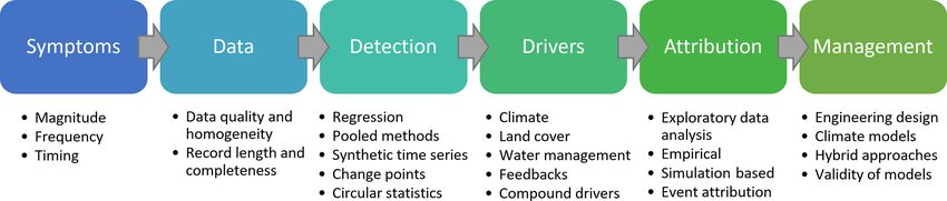
L. J. Slater et al.: Nonstationary weather and water extremes: a review                                                                  3903

Figure 4. Examples of trends in magnitude, frequency, and timing of hydroclimatic extremes. (a) Trends in extreme daily precipitation
frequency (left plot – events) and magnitude (right plot – annual mean extreme daily precipitation anomaly; millimetres) over the globe
(Papalexiou and Montanari, 2019). (b) Trend in the temperature anomaly of the highest temperature of the year (degrees Celsius) over the
globe (baseline period – 1970–1989); the red line indicates 5-year moving average (Papalexiou et al., 2018). (c) Trends in flood timing across
Europe in days per decade, 1960–2010 (Blöschl et al., 2017). (d) Trends in the magnitude of 20-year river floods, 1970s–present (Slater et al.,
2021). (e) Global trends in wind speed. The left map shows the linear trend in metres per second per decade of ERA-Interim 90th percentile
of 10 m wind speed for December–February (DJF; significant trends hatched). The right map shows the 850 hPa wind speed trends produced
by ERA-I, JRA-55 and MERRA-2, where blues (reds) indicate the level of agreement between reanalyses about negative (positive) trends
(Torralba et al., 2017).

https://doi.org/10.5194/hess-25-3897-2021                                               Hydrol. Earth Syst. Sci., 25, 3897–3935, 2021
3904                                                    L. J. Slater et al.: Nonstationary weather and water extremes: a review

proaches more complicated to implement than block max-                est in the nonstationarity of IDF curves (Cheng and AghaK-
ima approaches, where only one extreme per block (unit of             ouchak, 2014; Ganguli and Coulibaly, 2017) and the impli-
time) is selected. More flexible selection of extremes and a          cations of this nonstationarity for compound hydroclimatic
larger sample size of frequency-based (i.e. POT) approaches           extremes globally (AghaKouchak et al., 2020).
may be preferred when record length is a limiting factor,
whereas simpler magnitude-based (i.e. block maxima) ap-               2.3   Timing
proaches may be preferred when longer records are available.
   More severe hydroclimatic extremes (such as 1 in 10-, 1 in         Nonstationarity in the timing and seasonality of weather and
20-, 1 in 50-, 1 in 100-, or 1 in 200-year events) are typically      water extremes has been examined far less than trends in
evaluated using return periods (or expected waiting time).            magnitude and frequency (see examples in Table 1). Timing
Alternatively, annual exceedance probabilities (AEPs) define          and seasonality provide information that is relevant for the
the probability that a threshold will be exceeded in a given          management of water resources and analysis of underlying
year. Other metrics have been proposed for engineering de-            drivers of change. For instance, the start of field operations
sign. Reviews by Salas et al. (2018) and François et al. (2019)       for farming may be estimated as the day of the year when
highlight ongoing disagreements about the utility of nonsta-          “the sum of average temperature from 1 January exceeds
tionary methods for the design of engineering structures. As          200 ◦ C” (e.g. Rivington et al., 2013; Harding et al., 2015).
the uncertainties of nonstationary model structures may ex-           Similarly, the start of the growing season may be measured
ceed that of stationary models (Serinaldi and Kilsby, 2015),          as the first of 5 consecutive days with average temperature
specific strategies are required to manage the consequences           exceeding 5 ◦ C (Rivington et al., 2013). Changes in these
of those uncertainties (François et al., 2019). There are, thus,      indicators of hydroclimatic extremes may have substantial
ongoing debates about which concepts and methods are most             impacts (e.g. crop yields). Additionally, changes in timing
appropriate for estimation of extremes, such as the return pe-        and seasonality can also affect the impacts of extreme events.
riod, risk, reliability or equivalent reliability (ER), design life   For example, the risk from compound tropical cyclones and
level (DLL) or average design life level (ADLL), and ex-              heatwaves is sensitive to the seasonal cycles in tropical cy-
pected number of exceedances (ENE; e.g. Read and Vogel,               clone probability (which peaks in late summer) and extreme
2015; Rootzén and Katz, 2013; Yan et al., 2017; Salas and             heat (midsummer). A greater frequency of tropical cyclones
Obeysekera, 2014). For instance, return period metrics may            earlier in summer, or more extreme heat late in summer,
exhibit limitations in the case of time-correlated hydroclima-        would increase the risk of compounding and attendant im-
tological extremes, so alternatives such as the equivalent re-        pacts (Matthews et al., 2019).
turn period (ERP; i.e. “the period that would lead to the same           Changes in the timing of seasonal streamflow are typically
probability of failure pertaining to a given return period T          assessed using the centre of volume (CV) date (Court, 1962)
in the framework of classical statistics, independent case”;          or mean date of flood occurrence (mean flood day – MFD).
Volpi et al., 2015) may be preferred.                                 For example, Hodgkins and Dudley (2006) assessed changes
   It is not just individual characteristics of weather and water     in flood timing over the conterminous USA from 1913–2002
extremes that can change over time but also the interdepen-           using the winter–spring CV dates. They found that a third
dence between different characteristics, such as frequency,           of stations north of 44◦ had significantly earlier flows, likely
magnitude, and volume. Myhre et al. (2019) highlight that,            related to changes in winter and spring air temperatures af-
in a warming climate, increases in extreme rainfall are likely        fecting winter snowpack. The MFD has been used to assess
to be driven by shifts in both the intensity and frequency of         changes in streamflow timing in specific countries such as
events, but increases in the frequency are most important.            Wales (Macdonald et al., 2010) and Spain (Mediero et al.,
Brunner et al. (2019) assessed future changes in flood peak           2014). Probabilistic methods for identifying flood seasonal-
volume dependencies and found that the interdependence be-            ity and their trends (Cunderlik et al., 2004) have been applied
tween variables may change more strongly than the individ-            in Canada (Cunderlik and Ouarda, 2009) and the northeast-
ual variables themselves. This interdependency also applies           ern United States (Collins, 2019). In Europe, an analysis of
to other variable pairs jointly of interest, such as drought du-      4262 streamflow stations in 38 countries used the date of oc-
ration and deficit or precipitation intensity and duration. Rec-      currence of the highest annual peak flow to assess changes
ognizing the interdependence between magnitude and fre-               in flood timing (Blöschl et al., 2017). This showed signifi-
quency, many studies employ intensity–duration–frequency              cant changes in the seasonal timing of floods at the regional
(IDF) metrics, which describe both the magnitude and fre-             scale. In northeastern Europe, 81 % of stations had shifted to-
quency at once. It has recently been shown that generalized           wards earlier floods (by 8 d per 50 years), in western Europe,
extreme value (GEV) distribution parameters scale robustly            50 % of stations had shifted towards earlier floods (by 15 d
with event duration at the global scale (R 2 > 0.88); hence, a        per 50 years), and around the North Sea, 50 % of the stations
universal IDF formula can be applied to estimate rainfall in-         had shifted towards later floods (by 8 d per 50 years), as seen
tensity for a continuous range of durations, including at the         in Fig. 4c (Blöschl et al., 2017). Wasko et al. (2020b) eval-
subdaily scale (Courty et al., 2019). There is growing inter-         uated global shifts in the timing of streamflow based on the

Hydrol. Earth Syst. Sci., 25, 3897–3935, 2021                                          https://doi.org/10.5194/hess-25-3897-2021
L. J. Slater et al.: Nonstationary weather and water extremes: a review                                                       3905

local water year and found that shifts in the timing of annual     density/cover, post-processing, and archiving (unit changes;
floods were 3 times greater than shifts in mean streamflow.        Wilby et al., 2017). For example, the England and Wales pre-
Furthermore, the drivers of streamflow timing depend on the        cipitation series is a specific example of spurious nonstation-
magnitude of the event; less extreme events tend to corre-         arity (a long-term trend towards wetter winters) arising from
spond with soil moisture timing, while more extreme events         a combination of climate drivers (cold winters with more
depend more on rainfall timing (Wasko et al., 2020a).              snowfall in the early 19th century) with non-standard rain
   Nonstationarity in the timing of extreme precipitation has      gauges before the mid-1860s and snowfall undercatch, giving
also been used to better understand the causal factors of ex-      an apparent increase in winter precipitation (Fig. 5a; Mur-
tremes. Gu et al. (2017) examined shifts in the seasonality        phy et al., 2020b). Gridded products and reanalysis data are
and spatial distribution of extreme rainfall over 728 stations     also not immune from such data quality issues and are fur-
in China and found that alterations in rainfall seasonality        ther affected by time–space variations in raw data inputs and
were likely being driven by changes in the pathways of sea-        version updates (Sterl, 2004; Ferguson and Villarini, 2014).
sonal vapour flux and tropical cyclones. Others have exam-            Detecting spurious nonstationarities within raw data
ined shifts in the seasonality of future large-scale global pre-   should be one of the first steps when evaluating time series
cipitation and temperature extremes from model projections         that have yet to be quality controlled. Approaches have been
such as the Climate Model Intercomparison Project (CMIP;           proposed for uncovering homogeneity issues (see Fig. 5b).
e.g. Zhan et al., 2020) (see Sect. 7.2 for a discussion of the     Common techniques for assessing data quality range from vi-
projections). For instance, Marelle et al. (2018) investigated     sual inspection or expert judgement to formal statistical tests
changes in the seasonal timing of extreme daily precipita-         (e.g. Chow test, Buishand range test, Pettitt test, and standard
tion using CMIP5 models for RCP8.5 (high future emissions          normal homogeneity tests). For meteorological variables, rel-
scenario) and found that, by the end of the 21st century, ex-      ative homogeneity tests are possible where appropriate net-
treme precipitation could shift from summer/early fall toward      works of observations are available (e.g. HOMER; Mestre
fall/winter, especially in northern Europe and northeastern        et al., 2013). However, such techniques are often limited to
America. Brönnimann et al. (2018) employed a large ensem-          evaluating changes in the mean rather than extremes (Peña-
ble of bias-corrected climate model simulations to under-          Angulo et al., 2020; Ribeiro et al., 2016; Yosef et al., 2019).
stand changes in Alpine precipitation and found the annual            An important step towards detecting and attributing non-
maximum 1 d precipitation events (Rx1day) became more              stationarity is providing better metadata about measurement
frequent in early summer and less frequent in late summer,         practice and any changes in observational techniques, as well
due to summer drying.                                              as guidance on basic quality assurance approaches and the
                                                                   procurement and servicing of data sets. Observations are the
                                                                   foundation for understanding hydroclimatic change. Unfor-
3     Data considerations before detecting and attributing         tunately, data sets of essential variables (precipitation, evap-
      nonstationarity                                              otranspiration, discharge, etc.) are typically disbursed across
                                                                   various global, regional, and national archives containing dif-
3.1    Spurious nonstationarities: the issue of data quality       ferent variables and timescales in varied formats. For stream-
                                                                   flow records, changes in the rating quality are rarely noted.
Confidence in nonstationarity detection, attribution, and pre-     Large, multi-country databases, such as the Global Runoff
diction rests on confidence in the homogeneity and quality of      Data Centre (GRDC; https://portal.grdc.bafg.de/, last access:
input data – including the primary hydrometeorological se-         6 July 2021), are vital for providing an overview of nonsta-
ries from individual observations, accompanying metadata,          tionarities at continental and global scales but do not pro-
and qualitative information. Data quality issues tend to be        vide information on streamflow data quality. Accordingly,
particularly prevalent with measurement of extremes. Hydro-        there are limitations on what can be said in global studies
climatologists increasingly need to be aware of data quality       when compared with local knowledge. There is recognition
issues associated with the homogeneity of remotely sensed          of the need to create integrated data sets of observed variables
data and their derivatives. For example, inaccuracies may          for understanding and detecting change (e.g. Thorne et al.,
arise from orbital drift (Weber and Wunderle, 2019), infer-        2017). The CAMELS (catchment attributes and meteorology
ence of precipitation from vegetation in data-sparse regions       for large sample studies) initiative is an excellent start in hy-
(Xu et al., 2015), or changing land surface reflectance such as    drology, as these resources provide large integrated hydro-
snow cover over mountainous regions (Karaseva et al., 2012).       logic data sets for regions of the world. CAMELS data sets
Some of the most common sources of data errors and biases          already exist for the USA (Addor et al., 2017), UK (Coxon
that reduce homogeneity or cause nonstationarity in ground-        et al., 2020), Australia (Fowler et al., 2021b), Brazil (Chagas
based information over timescales of years to decades are          et al., 2020), and Chile (Alvarez-Garreton et al., 2018).
site or instrument changes, biases and drift in field proce-
dures (time of sample and preferred values), unstable rat-
ing curves and channel cross sections, changes in network

https://doi.org/10.5194/hess-25-3897-2021                                       Hydrol. Earth Syst. Sci., 25, 3897–3935, 2021
3906 L. J. Slater et al.: Nonstationary weather and water extremes: a review
Figure 5. Homogeneity of observational records. (a) An example of spurious nonstationarity in mean observed (red line) winter precipitation
for England and Wales due to inhomogeneous records. The ensemble median and individual reconstructions (black and grey lines) do not
exhibit nonstationarity (from Murphy et al., 2020b). (b) An approach to data homogenization for monthly to annual climate records (adapted
from Aguilar et al., 2003).
3.2 Record length and completeness 2016), with some attributing this decline and correspond-
ing increase in drought frequency to anthropogenic forcing
in the Mediterranean basin (e.g. Barkhordarian et al., 2013;
The observed record length required for assessments of non- Gudmundsson and Seneviratne, 2016; Hoerling et al., 2012).
stationarity depends on the type of process under consid- However, when viewed in the context of rescued and quality
eration, the aims of analysis, properties of the underlying assured data beginning in the mid-19th century, these recent
data, as well as the timescales of the sources of nonstation- trends in precipitation are within the range of longer-term
arity (drivers of change). For instance, Atlantic sea surface variability (Vicente-Serrano et al., 2019). Without sufficient
temperatures (SSTs) vary over periods longer than 50 years record length, false attribution statements may arise with po-
(McCarthy et al., 2015; Sutton and Dong, 2012) and affect tentially significant management implications.
concurrent precipitation and temperature patterns. The North The challenges posed by the lack of available long-term
Atlantic was particularly cold during the middle of the cli- observations have prompted some to leverage advances in
mate normal period (1961–1990) due to the Atlantic Multi- data rescue and historical climatology to extend discharge
decadal Oscillation or great saline anomaly (Dickson et al., series back in time (e.g. O’Connor et al., 2020; Smith et al.,
1988). Hence, even 50 years of data are insufficient to ro- 2017; Bonnet et al., 2020). Palaeo-hydroclimatic reconstruc-
bustly detect true nonstationarities because the start and end tions are also employed to extend data back in time and
dates of records may substantially affect the sign (direction) provide greater insight into current conditions. For example,
and magnitude of trends (Harrigan et al., 2018), especially warm and cool season rainfall was reconstructed in Australia
in records that exhibit multi-decadal periodicity. Hundreds to investigate the recent observed trend magnitude in the con-
of years are required to adequately identify certain stationary text of palaeoclimatic variability (Freund et al., 2017). Hy-
models (Thyer et al., 2006), let alone nonstationary models. droclimatic reconstructions of the last 500 years have consid-
Additionally, highly variable time series require a larger per- erable potential to place recent observations into a long-term
centage change in the mean of the data to identify a statisti- context that is not achievable from short observation-based
cally significant change compared with less variable time se- record lengths alone. Although such data sets lengthen the
ries (e.g. Chiew and McMahon, 1993). In places where series period available for analysis and better reflect ranges of vari-
have low signal-to-noise ratios, the time required to detect ability in extremes such as drought (Murphy et al., 2020a),
plausible trends (e.g. in precipitation, evapotranspiration, and they are subject to limitations from changes in measurement
discharge extremes) can, thus, be centuries long (e.g. Ziegler practice, decreasing density of observations in early records,
et al., 2005; Wilby, 2006). In some cases, faster detection and a lack of consideration of issues such as changes in land
may be possible using seasonal, rather than annual, time se- cover and shifts in channel capacity (Slater et al., 2015).
ries (e.g. Ziegler et al., 2005). In many regions, temporal and spatial data sparsity is
The mismatch between the temporal scales of drivers of likely to remain a key issue, hindering robust detection, attri-
climate variability versus the availability and quality of ob- bution, and prediction of water and climate nonstationarities.
servations can also result in misleading conclusions. For Therefore, different trend detection and attribution methods
example, numerous studies have reported decreasing pre- should be considered (e.g. using lower quantiles and peak
cipitation in Mediterranean regions since the 1960s (Lon- over threshold methods; see Sect. 4), while implementing
gobardi and Villani, 2010; Gudmundsson and Seneviratne,
Hydrol. Earth Syst. Sci., 25, 3897–3935, 2021 https://doi.org/10.5194/hess-25-3897-2021L. J. Slater et al.: Nonstationary weather and water extremes: a review 3907
holistic “multiple working hypotheses” approaches (Cham- 1994) has often been used alongside MK (e.g. Hannaford
berlin, 1890; Harrigan et al., 2014) to avoid overlooking po- et al., 2021) to estimate the magnitude of the trend over time
tential drivers of change. Finally, gaps in extreme hydrocli- (as the median slope of all paired values in the record). Dif-
matic time series may also affect the detection rate of signif- ferent versions of the MK test exist to detect seasonal and
icant trends. Detection rates are lower in records that have regionally coherent trends over time (see Helsel et al., 2020,
larger gaps and shorter length than those with less change for details and examples).
(lower regression slopes) and fewer gaps and/or when the Other studies also apply ordinary least square (OLS) linear
data gaps are located towards the beginning or end of a time regression to estimate trends in precipitation (e.g. Fig. 4a; Pa-
series (Slater and Villarini, 2017a). palexiou and Montanari, 2019), temperature (e.g. Papalexiou
et al., 2018), and flood flows (e.g. Hecht and Vogel, 2020).
Practical advantages for using OLS methods include the ease
4 Detection of nonstationarity of use and expression of uncertainty, graphical communica-
tion, and usability for providing decision-relevant informa-
Detection of nonstationarity in hydroclimatological extremes tion (e.g. Hecht and Vogel, 2020). In cases where the as-
requires a sound examination of the data before applying any sumptions of OLS are not met (such as linearity, indepen-
statistical tests which broadly seek to detect the following dence, normality, and equal variance of the residuals), non-
two types of nonstationarity (see Fig. 1b): monotonic change parametric alternatives such as the Theil–Sen slope estimator
(trends) and step changes (change points). Such changes can or quantile regression (QR) may be used (both trend lines can
be considered as symptoms of nonstationarity if they rep- be plotted). Instead of estimating the conditional mean of the
resent a significant departure from normality within a long- response variable, QR considers different conditional quan-
term record. Nonstationarity may be detected either in indi- tiles (including the median) of a distribution. QR has been
vidual time series (point-based analysis) or in larger ensem- used for precipitation trends (e.g. Tan and Shao, 2017), air
bles of stations (spatially coherent trends; Hall et al., 2014). temperature (e.g. Barbosa et al., 2011), surface wind speed
Here, we provide an overview of existing methods employed (e.g. Gilliland and Keim, 2018), and flood trends (e.g. Villar-
in the fields of weather and water extremes. For a descrip- ini and Slater, 2018) and is also regularly employed to inves-
tion of change detection methods in hydrology, we refer the tigate scaling properties between hydroclimatological vari-
reader to Helsel et al. (2020) and, for floods, to Villarini et al. ables (see Sect. 5.1; e.g. Wasko and Sharma, 2014).
(2018). For an overview of methods and challenges in the When the empirical distribution of hydroclimatic extremes
detection and attribution of climate extremes, see Easterling is known, many prefer to select an appropriate distribution
et al. (2016). and evaluate how the distribution parameters vary as a func-
tion of covariates such as time (e.g. Katz, 2013). For exam-
4.1 Regression-based methods for detection of ple, the nonstationary generalized extreme value (GEV) or
incremental change Gumbel (GU) distributions are widely used to detect trends
in annual or seasonal maxima such as floods (e.g. Prosdocimi
The detection of trends in hydroclimatic time series gener- et al., 2015), precipitation (e.g. Gao et al., 2016), and wind
ally employs the following two key approaches: detection of (e.g. Hundecha et al., 2008), while the Poisson (PO; e.g. Neri
trends in magnitude (e.g. quantiles or block maxima, such et al., 2019) or negative binomial (NBO; e.g. Khouakhi et al.,
as the annual maxima, AMAX) or frequency-based methods 2019) distributions are preferred for discrete data (e.g. counts
(e.g. use of point process modelling frameworks to model the of days over thresholds). These distributions can be fitted to
peaks over threshold (POT) series, also referred to as partial- the data either with constant parameters (stationary case) or
duration series (PDS; e.g. Coles, 2001; Salas et al., 2018). with the parameters expressed as a function of time (nonsta-
The non-parametric Mann–Kendall (MK) test (Mann, tionary case; Katz, 2013).
1945; Kendall, 1975) is a distribution-free test frequently em- In the nonstationary case, a time or climate covariate can
ployed to detect monotonic trends in time series without as- be employed to detect changes in the parameters of the distri-
suming a linear trend. Instead, MK simply evaluates whether bution, as illustrated in Fig. 6. The advantage of employing
the central tendency or median of the distribution changes climate covariates is that climate model predictions or pro-
monotonically over time (see Helsel et al., 2020). The test jections can then be employed as covariates to estimate future
statistic, Kendall’s τ , is a rank correlation coefficient which change (as discussed in Sect. 7.3; e.g. Du et al., 2015). Crite-
ranges from −1 to +1. For instance, Westra et al. (2013) ria for model selection, such as the Akaike information crite-
evaluated trends in annual maximum daily precipitation at rion (AIC) or Schwarz Bayesian criterion (SBC; also known
8326 precipitation stations with at least 30 years of records as the Bayesian information criterion – BIC) can then be used
and found increases at approximately two-thirds of these sta- to determine whether the stationary or nonstationary model
tions. A modified version of the MK test can also be applied is the better fit (e.g. Fig. 6a). The AIC and BIC assess the
to autocorrelated data (Hamed, 2009a, b). The Theil–Sen trade-off between goodness of fit and model complexity, so
slope estimator (Sen, 1968; Theil, 1992; Hipel and McLeod, the improvement in the goodness of fit must be sufficient to
https://doi.org/10.5194/hess-25-3897-2021 Hydrol. Earth Syst. Sci., 25, 3897–3935, 20213908 L. J. Slater et al.: Nonstationary weather and water extremes: a review
overcome the complexity penalty. Small differences in AIC tion of global changes in 20-year river floods since the 1970s
are not always meaningful, such that several models may be found a majority of increases in temperate climates but de-
equally acceptable (e.g. Wagenmakers and Farrell, 2004). In creases in cold, polar, arid, and tropical climates (Fig. 4d;
cases where the nonstationary model performs significantly Slater et al., 2021). Importantly, the covariate in a GAMLSS
better than a stationary model (in terms of goodness of fit and nonstationary model is often time (e.g. Villarini et al., 2009a;
uncertainty), then the time series may be considered as non- Serinaldi and Kilsby, 2015) but may also include other phys-
stationary, pending sufficient record length (see Sect. 3.2). ical drivers such as climate modes (e.g. Villarini and Seri-
Increasingly, distributional regression modelling frame- naldi, 2012), urban or agricultural land cover (e.g. Villarini
works, such as vector generalized linear and additive mod- et al., 2009b; Slater and Villarini, 2017b), or other hydrocli-
els (VGLM and VGAM, respectively) or generalized addi- matic variables such as dew point temperature (e.g. Lee et al.,
tive models for location, scale, and shape (GAMLSS), are 2020).
being chosen for their flexibility in evaluating the nonstation- Finally, there is growing interest in using interpretable ma-
arity of hydroclimatic extremes (e.g. Serinaldi and Kilsby, chine learning methods for detection of nonstationarities in
2015). These frameworks are a generalization of generalized weather and water extremes. For example, Prophet (Taylor
linear models (GLMs) that allow a broader range of distri- and Letham, 2018) is a decomposable time series forecast-
butions and different relationships between parameters and ing model, similar to generalized additive models (GAMs;
explanatory variables (linear, nonlinear, or smooth nonpara- Hastie and Tibshirani, 1987), which is increasingly popu-
metric). GAMLSS models, for instance, can have up to four lar for hydroclimatological time series modelling. For exam-
parameters, i.e. µ, σ , ν, and τ , which allow for the modelling ple, Papacharalampous and Tyralis (2020) used the model for
of the location (mean, median, and mode), scale (spread in forecasting mean annual discharge 1 year ahead, and Aguil-
terms of the standard deviation and coefficient of variation) era et al. (2019) used the approach for groundwater-level
and shape (skewness and kurtosis) of a distribution. An ex- forecasting. Prophet decomposes the time series into a trend
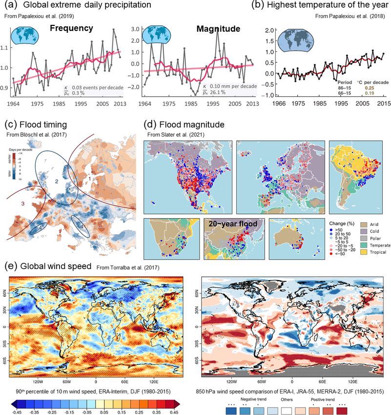
ample of nonstationarity detection is shown in Fig. 6. Here, component and a seasonal or periodic component, such as
two nonstationary (with time-varying parameters) and two annual or daily cycles. The trend component is a piecewise
stationary (constant parameters) models are fitted using both linear growth model, meaning that, for each partition (piece)
the Gamma and Weibull distributions to observed time se- of the time series (separated by the change points), the model
ries of instantaneous (15 min) peak maxima (Fig. 6a). In the fits a unique trend (varying the trend over time), and the pe-
nonstationary case, the (µ and σ ) model parameters both de- riodic effects are modelled as a Fourier series. This approach
pend linearly on the time covariate (in years). A logarithmic allows users to determine the locations in time when there
link function is employed to ensure the distribution param- are significant changes.
eters remain positive. The goodness of fit of both stationary
and nonstationary models is assessed using SBC (Fig. 6a). A 4.2 Pooled methods for detecting changes in extremes
detrended quantile–quantile (worm) plot showing the resid-
uals for different ranges of the explanatory variable(s) can As noted above, trend detection of hydroclimatic extremes
also be used to diagnose model fit (Fig. 6b). The model fit is problematic when there is uncertainty arising from short
is satisfactory if the worm is relatively flat and if data points record lengths or small samples. Extreme events such as the
lie within the confidence intervals. In the case of the River annual maximum, or 1 in n (50 or 100)-year events, tend to be
Ouse, we find the nonstationary Gamma model is the best- highly variable and require lengthy time series to ensure ro-
fitting model. However, the Gamma and Weibull nonstation- bust detection of significant nonstationarities. In cases where
ary model fits are fairly similar (Fig. 6a), and if the worm the sample size of observed records is insufficient, alternative
plots indicate a similar goodness of fit, it may well be that methods have been proposed, ranging from pooled sampling
both are acceptable, but the Gamma nonstationary model is to scaling approaches.
simply slightly better. Here, both the µ and σ parameters are Various pooled methods can be used to address the issue
increasing over time (Fig. 6c, d). The 50-year flood (spe- of limited sample size over large spatial scales. One pooled
cific discharge) increased from 0.123 m3 /s/km2 in 1900 to approach is to extract the single largest event over an n-year
0.183 m3 /s/km2 in 2018 (Fig. 6f). period from multiple independent gauge-based records, ef-
GAMLSS methods have been applied for different hy- fectively substituting space (large spatial sample across many
droclimatic extremes. For example, Bazrafshan and Hejabi gauges) for time (long temporal sample at individual gauges).
(2018) developed a nonstationary reconnaissance drought in- In other words, by pooling the data from multiple records
dex (NRDI) to assess drought nonstationarity in Iran and or data sets, the data sample is increased for greater statisti-
found large differences between the NRDI and a traditional cal robustness. For instance, Berghuijs et al. (2017) assessed
RDI (reconnaissance drought index) for time frames longer changes in 30-year floods across multiple continents by not-
than 6 months. Sun et al. (2020b) also evaluated changes ing the date of occurrence of the single largest daily stream-
in a nonstationary standardized runoff index (NSRI) using flow at individual gauges and by evaluating the fraction of
GAMLSS over the Heihe River basin in China. An evalua- catchments experiencing their maximum flood at different
Hydrol. Earth Syst. Sci., 25, 3897–3935, 2021 https://doi.org/10.5194/hess-25-3897-2021You can also read