North Atlantic Oscillation response in GeoMIP experiments G6solar and G6sulfur: why detailed modelling is needed for understanding regional ...
←
→
Page content transcription
If your browser does not render page correctly, please read the page content below
Atmos. Chem. Phys., 21, 1287–1304, 2021
https://doi.org/10.5194/acp-21-1287-2021
© Author(s) 2021. This work is distributed under
the Creative Commons Attribution 4.0 License.

North Atlantic Oscillation response in GeoMIP experiments G6solar
and G6sulfur: why detailed modelling is needed for understanding
regional implications of solar radiation management
Andy Jones1 , Jim M. Haywood1,2 , Anthony C. Jones3 , Simone Tilmes4 , Ben Kravitz5,6 , and Alan Robock7
1 Met Office Hadley Centre, Exeter, EX1 3PB, UK
2 Global Systems Institute, College of Engineering, Mathematics and Physical Sciences, University of Exeter,
Exeter, EX4 4QE, UK
3 Met Office, Exeter, EX1 3PB, UK
4 Atmospheric Chemistry, Observations and Modeling Laboratory, National Center for Atmospheric Research,

Boulder, CO 80307, USA
5 Department of Earth and Atmospheric Sciences, Indiana University, Bloomington, IN 47405-1405, USA
6 Atmospheric Sciences and Global Change Division, Pacific Northwest National Laboratory, Richland, WA 99352, USA
7 Department of Environmental Sciences, Rutgers University, New Brunswick, NJ 08901-8551, USA

Correspondence: Andy Jones (andy.jones@metoffice.gov.uk)

Received: 31 July 2020 – Discussion started: 17 August 2020
Revised: 3 December 2020 – Accepted: 13 December 2020 – Published: 29 January 2021

Abstract. The realization of the difficulty of limiting global-   nent and leading to high-latitude warming over Europe and
mean temperatures to within 1.5 or 2.0 ◦ C above pre-             Asia. These results are broadly consistent with previous find-
industrial levels stipulated by the 21st Conference of Parties    ings which show similar impacts from stratospheric volcanic
in Paris has led to increased interest in solar radiation man-    aerosol on the NAO and emphasize that detailed modelling
agement (SRM) techniques. Proposed SRM schemes aim                of geoengineering processes is required if accurate impacts
to increase planetary albedo to reflect more sunlight back        of SRM effects are to be simulated. Differences remain be-
to space and induce a cooling that acts to partially offset       tween the two models in predicting regional changes over the
global warming. Under the auspices of the Geoengineering          continental USA and Africa, suggesting that more models
Model Intercomparison Project, we have performed model            need to perform such simulations before attempting to draw
experiments whereby global temperature under the high-            any conclusions regarding potential continental-scale climate
forcing SSP5-8.5 scenario is reduced to follow that of the        change under SRM.
medium-forcing SSP2-4.5 scenario. Two different mecha-
nisms to achieve this are employed: the first via a reduction
in the solar constant (experiment G6solar) and the second via
modelling injections of sulfur dioxide (experiment G6sulfur)      1   Introduction
which forms sulfate aerosol in the stratosphere. Results from
two state-of-the-art coupled Earth system models (UKESM1          Successive Intergovernmental Panel on Climate Change
and CESM2-WACCM6) both show an impact on the North                (IPCC) reports (e.g. Forster et al., 2007; Myhre et al., 2013)
Atlantic Oscillation (NAO) in G6sulfur but not in G6solar.        have highlighted that anthropogenic greenhouse gas emis-
Both models show a persistent positive anomaly in the NAO         sions exert a strong positive radiative forcing, leading to a
during the Northern Hemisphere winter season in G6sulfur,         warming of Earth’s climate. However, the same IPCC re-
suggesting an increase in zonal flow and an increase in North     ports also suggest that aerosols of anthropogenic origin exert
Atlantic storm track activity impacting the Eurasian conti-       a significant (but poorly quantified) negative radiative forc-
                                                                  ing, leading to a cooling effect on the Earth’s climate through

Published by Copernicus Publications on behalf of the European Geosciences Union.
1288                   A. Jones et al.: North Atlantic Oscillation response in GeoMIP experiments G6solar and G6sulfur

aerosol–radiation and aerosol–cloud interactions. Aerosols         residual impacts of SAI such as the overcooling of the trop-
have therefore been at the forefront of discussions about          ics and undercooling of polar latitudes that are evident un-
increasing planetary albedo by deliberate injection either         der more generic SAI strategies (e.g. MacMartin et al., 2013;
into the stratosphere (stratospheric aerosol intervention, SAI;    Tilmes et al., 2018). However, studies suggest that SAI would
Dickinson, 1996) or into marine boundary layer clouds (ma-         by no means ameliorate all effects of climate change (e.g.
rine cloud brightening, MCB; e.g. Latham, 1990). Such pu-          Simpson et al., 2019; Da-Allada et al., 2020; Robock, 2020).
tative albedo-increasing interventions are referred to as solar       The North Atlantic Oscillation (NAO) can be defined as a
radiation management (SRM) geoengineering.                         change in the pressure difference between the Icelandic Low
   Initial simulations of the impacts of SAI and MCB were          and the Azores High pressure regions (e.g. Hurrell, 1995),
carried out by individual groups using models of varying           and by convention, a positive NAO anomaly is associated
complexity for a range of different scenarios, but the range       with an increase in the surface pressure gradient between
of different scenarios applied to the models meant that defini-    these regions. Both model simulations (e.g. Stenchikov et
tive reasons for differences in model responses were difficult     al., 2002) and observations (e.g. Graf et al., 1994; Kodera,
to establish (e.g. Rasch et al., 2008; Jones et al., 2010). The    1994; Lorenz and Hartmann, 2003) have shown that one of
Geoengineering Model Intercomparison Project (GeoMIP)              the most significant atmospheric responses following explo-
framework was therefore established with specific proto-           sive volcanic eruptions is a strengthening of the polar vor-
cols for performing model simulations under a range of de-         tex and an impact on the Northern Hemisphere wintertime
fined scenarios (Kravitz et al., 2011). The scenarios con-         NAO, although in the case of the 1991 Pinatubo eruption
sidered by GeoMIP have themselves evolved with the ear-            the causal link has recently been questioned by Polvani et
liest idealized simulations being supplemented by progres-         al. (2019). Shindell et al. (2004) provide a concise sum-
sively more complex scenarios aiming to address more spe-          mary of the mechanism by which volcanic stratospheric
cific policy-relevant questions. The earliest simulations in-      aerosols are thought to influence the dynamical response
volved balancing an abrupt quadrupling of atmospheric car-         of the NAO, leading to wintertime warming over Eurasia
bon dioxide concentrations by simply reducing the solar con-       and North America (Robock and Mao, 1992). Essentially,
stant (GeoMIP experiment G1; Kravitz et al., 2011). While          (1) sunlight absorbed by aerosols leads to heating of the
such simulations are highly idealized, the simplicity of the       lower stratosphere, which enhances the meridional tempera-
scenario means that many climate models could perform              ture gradient; (2) this leads to a strengthening of the westerly
the simulations, providing a robust multi-model assessment         zonal winds near the tropopause; (3) planetary waves prop-
(Kravitz et al., 2013, 2020).                                      agating upwards in the troposphere are refracted away from
   Policy-relevant questions regarding SRM can only be ad-         the pole due to the change in wind shear, further strength-
dressed by climate model simulations that represent deploy-        ening the westerlies; (4) the enhanced westerlies propagate
ment strategies which use technologies that are considered         down to the surface via a positive feedback between the zonal
safe, cost-effective and have a reasonably short development       wind anomalies and tropospheric eddies; and (5) strength-
time (Royal Society, 2009). SAI has been suggested as one          ened westerly flow near the ground creates the surface pres-
such potentially plausible mechanism; its plausibility is en-      sure and temperature response patterns. As SAI geoengineer-
hanced by observations of explosive or effusive volcanic           ing could be considered equivalent to a continuous volcanic
eruptions which cause a periodic negative radiative forcing        eruption, it seems plausible that it too could generate similar
and a cooling of the Earth’s climate (e.g. Robock, 2000; Hay-      anomalies in the NAO and so surface temperature.
wood et al., 2013; Santer et al., 2014; Malavelle et al., 2017).      In addition to work on the dynamical features and NAO
Observations of such natural analogues provide powerful            response to SAI via volcanic eruptions, there has been much
constraints on the ability of global climate models to repre-      debate on the influence of the 11-year solar cycle with
sent complex aerosol–radiation and aerosol–cloud processes,        stronger solar activity being associated with a positive phase
although the pulse-like nature of the emissions from volcanic      of the NAO and weaker solar activity being associated with
eruptions means that they are not perfect analogues for SRM        a negative phase. Early work (e.g. Kodera, 2002; Kodera and
(Robock et al., 2013). Single model simulations which in-          Kuroda, 2005; Matthes et al., 2006) suggested that mech-
clude treatments of aerosol processes associated with SAI          anisms influencing the NAO from solar variability origi-
(e.g. Jones et al., 2017, 2018; Irvine et al., 2019) have shown    nated near the stratopause, propagated downward through
that policy-relevant climate metrics at global, continental and    the stratosphere and influenced the troposphere via changes
regional scales such as sea-level rise, sea-ice extent, Euro-      in meridional propagation of planetary waves. More recent
pean heat waves, Atlantic hurricane frequency and intensity,       work has suggested that stronger correlations exist between
and North Atlantic storm track displacement can be signifi-        the solar cycle and the phase and strength of the NAO if a
cantly ameliorated under SAI geoengineering compared with          lag is accounted for (Gray et al., 2013), owing to ocean–
baseline (non-geoengineered) scenarios. Additionally, SAI          atmosphere interactions that strengthen the response (Scaife
strategies could potentially be tailored to provide spatial dis-   et al., 2013). These lagged responses to solar cycles have
tributions of stratospheric aerosol that mitigate some of the      been replicated in some climate models (e.g. Ineson et al.,

Atmos. Chem. Phys., 21, 1287–1304, 2021                                              https://doi.org/10.5194/acp-21-1287-2021
A. Jones et al.: North Atlantic Oscillation response in GeoMIP experiments G6solar and G6sulfur                              1289

2011), including a version of the model that was the forerun-      periments. Results are presented in Sect. 4 before discussions
ner of the UKESM1 model that is used in our analysis (see          and conclusions are presented in Sect. 5.
Sect. 2).
   Stratospheric aerosol and the 11-year solar cycle are
not the only phenomena to influence the NAO: Smith et              2   Model description
al. (2016) indicate that Atlantic sea-surface temperatures, the
                                                                   Both UKESM1 and CESM2-WACCM6 are fully coupled
phase and strength of El Niño, the quasi-biennial oscillation,
                                                                   Earth system models which have contributed to CMIP6 and
Atlantic multi-decadal variability, and Pacific decadal vari-
                                                                   GeoMIP6. Both models (or their immediate forebears) have
ability may all play a role. However, skilful predictions of
                                                                   undergone various degrees of validation relevant to SAI
the wintertime NAO index using sophisticated seasonal pre-
                                                                   using observations from explosive volcanic eruptions (e.g.
diction models that account for these factors are now possi-
                                                                   Haywood et al., 2010; Dhomse et al., 2014; Mills et al.,
ble (Dunstone et al., 2016). Note that the two driving mech-
                                                                   2016).
anisms investigated in this study, i.e. SAI and a reduction
                                                                      UKESM1 is described by Sellar et al. (2019). It comprises
in solar constant, may induce opposing impacts on the NAO:
                                                                   an atmosphere model based on the Met Office Unified Model
SAI might strengthen the NAO, while reducing the solar con-
                                                                   (UM; Walters et al., 2019; Mulcahy et al., 2018) with a res-
stant might weaken it.
                                                                   olution of 1.25◦ latitude by 1.875◦ longitude with 85 levels
   The most recent GeoMIP Phase 6 scenarios (GeoMIP6;
                                                                   up to approximately 85 km, coupled to a 1◦ resolution ocean
Kravitz et al., 2015) attempt to provide more policy-relevant
                                                                   model with 75 levels (Storkey et al., 2018). It includes com-
information on SRM geoengineering by aligning with the
                                                                   ponents to model tropospheric and stratospheric chemistry
Coupled Model Intercomparison Project Phase 6 (CMIP6;
                                                                   (Archibald et al., 2020) and aerosols (Mann et al., 2010), sea
Eyring et al., 2016). Two GeoMIP6 experiments will be
                                                                   ice (Ridley et al., 2018), the land surface and vegetation (Best
considered here: G6solar and G6sulfur. In both experiments
                                                                   et al., 2011), and ocean biogeochemistry (Yool et al., 2013).
the modelled global-mean temperature under a high-forcing
                                                                      CESM2-WACCM6 is described by Danabasoglu et
scenario is reduced to that in a medium-forcing scenario.
                                                                   al. (2020) and Gettelman et al. (2019a). The atmosphere
The mechanism for performing the temperature reduction
                                                                   model has a resolution of 0.95◦ in latitude by 1.25◦ in longi-
is either an idealized reduction of the solar constant (ex-
                                                                   tude with 70 levels from the surface to about 140 km. This is
periment G6solar) or a more realistic injection of sulfur
                                                                   coupled to an ocean model component with a nominal 1◦ res-
dioxide into the stratosphere (experiment G6sulfur) where
                                                                   olution and 60 vertical levels (Danabasoglu et al., 2012) and
it forms sulfate aerosol that reflects sunlight back to space.
                                                                   a sea-ice model (Hunke et al., 2015). It includes a full strato-
We examine results from two Earth system models which
                                                                   spheric chemistry scheme that is coupled to the atmospheric
have performed both experiments (UKESM1 and CESM2-
                                                                   dynamics, aerosol and radiation schemes (Mills et al., 2017),
WACCM6). The main objective is to determine whether, un-
                                                                   and a land model with interactive carbon and nitrogen cycles
der SRM strategies which are continuous rather than spo-
                                                                   (Danabasoglu et al., 2020).
radic or periodic in nature, the two models produce NAO
responses that are consistent with the expectations discussed
above, i.e. that SAI induces a significant shift to the positive   3   G6solar and G6sulfur experimental design
phase of the NAO compared with reducing the solar con-
stant. Our analysis focuses on the broad-scale microphysi-         As described in Kravitz et al. (2015), the goal of GeoMIP
cal, chemical and dynamical features in the Northern Hemi-         experiments G6solar and G6sulfur is to modify simula-
sphere winter, i.e. aerosol spatial distributions, impacts on      tions based on ScenarioMIP high-forcing scenario SSP5-8.5
ozone, stratospheric temperatures, stratospheric and tropo-        (O’Neill et al., 2016; experiment ssp585) so as to follow
spheric zonal mean winds, and induced surface pressure pat-        the evolution of the medium-forcing scenario SSP2-4.5 (ex-
terns with a focus on the NAO, before examining impacts on         periment ssp245). Kravitz et al. (2015) define the criterion
continental-scale temperature and precipitation patterns. SAI      for comparing the modified simulations with their ssp245
is considered the most plausible SRM method, owing to con-         target in terms of radiative forcing. This was subsequently
siderations of effectiveness, timeliness, cost and safety (e.g.    found to be impractical for some models, so for GeoMIP6
Royal Society, 2009). Our focus is therefore on the difference     the criterion applied was that for each decade from 2021 to
between the responses to SRM via SAI and that via generic          2100 the global decadal-mean near-surface air temperature
reductions in the solar constant, noting that many previous        of G6solar or G6sulfur should be within 0.2 K of the corre-
assessments of the impacts of SRM use a reduction of the           sponding decade of each model’s ssp245 simulation. Experi-
solar constant as a proxy for SAI.                                 ment G6solar performs the required modification in an ideal-
   Section 2 provides a brief description of the UKESM1 and        ized manner by gradually reducing the solar constant over the
CESM2-WACCM6 models. Section 3 provides a description              21st century, whereas G6sulfur achieves it by the arguably
of the experimental design of the G6solar and G6sulfur ex-         more technologically feasible method of injecting gradually
                                                                   increasing amounts of SO2 into the lower stratosphere. SO2

https://doi.org/10.5194/acp-21-1287-2021                                            Atmos. Chem. Phys., 21, 1287–1304, 2021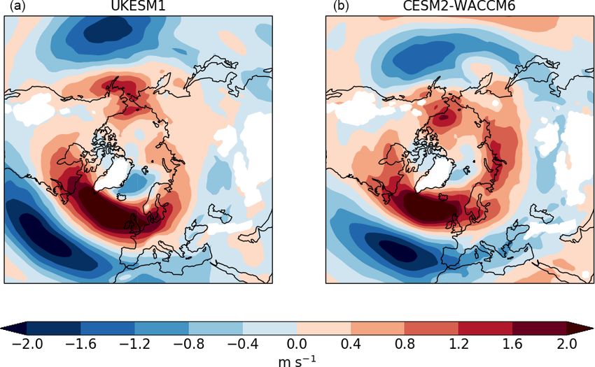
1290 A. Jones et al.: North Atlantic Oscillation response in GeoMIP experiments G6solar and G6sulfur
was injected continuously between 10◦ N–10◦ S along the ing is around 2.6 K compared with present day, while for
Greenwich meridian at 18–20 km altitude in UKESM1 and CESM2-WACCM6 the warming is more moderate at around
on the Equator at the date line at ∼ 25 km altitude in CESM2- 1.9 K. This result is interesting in itself because the base
WACCM6. models that are used in these simulations have been diag-
The results presented are ensemble means of three nosed as having equilibrium climate sensitivities (i.e. for a
(UKESM1) or two (CESM2-WACCM6) members. These doubling of CO2 ) of 5.4 K (UKESM1; Andrews et al., 2019)
are ultimately initial condition ensembles: the G6solar and and 5.3 K (CESM2; Gettelman et al., 2019b); one might thus
G6sulfur ensemble members are based on ensemble mem- expect a similar transient climate response under the SSP2-
bers of each model’s ssp585 experiment, which are them- 4.5 scenario.
selves continuations of corresponding CMIP6 historical sim- Both models warm over land regions more than over
ulations, which in turn are initialized from different points in ocean regions as documented in successive IPCC reports
each model’s pre-industrial control simulation. (e.g. Forster et al., 2007; Myhre et al., 2013). UKESM1
We investigate the impact of SAI by examining differ- shows a strong polar amplification, particularly in the North-
ences between G6sulfur and G6solar, generally over the fi- ern Hemisphere, while polar amplification is more muted
nal 20 years of the 21st century. We are thereby compar- in CESM2-WACCM6. This is likely linked to differences
ing two experiments in which the temperature evolution is in poleward atmospheric and oceanic heat transport. Indeed,
nominally the same, but they achieve this by different meth- CESM2-WACCM6 suggests that areas of the North Atlantic
ods. This should highlight any impacts which are captured are subject to a cooling as the mean climate warms. This
by a more detailed treatment of modelling SAI geoengineer- is presumably as a result of a strong reduction of the At-
ing (G6sulfur) which are not seen when geoengineering is lantic Meridional Overturning Circulation, which has been
treated in a more idealized fashion (G6solar). documented to collapse in CESM2 from a present-day level
of ∼ 23 to ∼ 8 Sv (sverdrup) by 2100 under the SSP5-
8.5 scenario (Muntjewerf et al., 2020; Tilmes et al., 2020).
4 Results UKESM1 shows no such behaviour.
The similarity between the inter-forcing patterns of tem-
We first provide a brief analysis of the levels of success perature responses in ssp245, G6solar and G6sulfur for each
that G6sulfur and G6solar have in reducing the temperature model is quite striking. On the basis of such an analysis, it
change to that of ssp245. As the experimental design assures would be tempting to conclude that G6solar, which has the
that the decadal-mean temperature in G6sulfur and G6solar benefits of being relatively simple to implement in a great
are within 0.2 K of the values for ssp245, we do not show the number of climate models (e.g. Kravitz et al., 2013, 2020),
temporal evolution of temperature, but there is some merit might be a reasonable analogue for the far more complex
in examining the inter-model and inter-forcing differences of G6sulfur simulations. This conclusion will be examined in
the resulting spatial patterns of temperature change to give the following sections.
context to the results that follow. When analysing the results
from the simulations, we generally focus on the difference 4.2 SO2 injection rate and aerosol optical depth
“G6sulfur minus G6solar” for several key variables that are
associated with our understanding of the influence of strato- In G6sulfur the mean SO2 injection rate during the final
spheric aerosol on the development of NAO anomalies. 2 decades (2081–2100) is 19.0 Tg yr−1 for UKESM1 and
20.6 Tg yr−1 for CESM2-WACCM6. Such injection rates are
4.1 Spatial distribution of 21st century temperature broadly similar to the amount injected by the 1991 eruption
change of Mt Pinatubo (Guo et al., 2004), but unlike the latter they
continue year on year. Such large, persistent perturbations
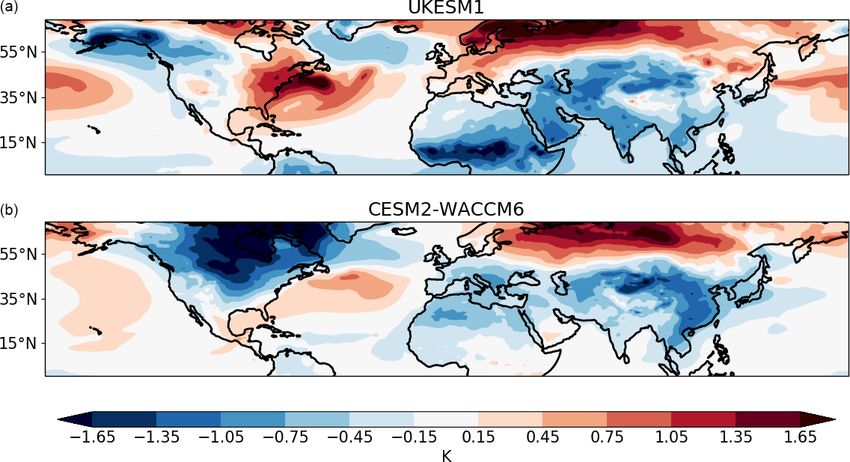
The spatial pattern of the global-mean temperature change are obviously different to the pulse-like injection and subse-
is calculated as the change from present day (PD; mean quent exponential decay of explosive volcanic eruptions (e.g.
of 2011–2030) compared with the period 2081–2100 and Jones et al., 2016a), which suggests that one cannot simply
is shown for experiments ssp245, G6solar and G6sulfur for assume that the responses to such SAI would be analogous to
UKESM1 and CESM2-WACCM6 in Fig. 1. PD data are from those from volcanic eruptions. The injection rates by the end
years 2011–2014 of each model’s CMIP6 historical experi- of the century have to be so large to counteract the warm-
ment combined with years 2015–2030 from the correspond- ing due to the increased concentration of atmospheric carbon
ing ssp245 experiment. dioxide which has accumulated over the period 1850–2100.
It is obvious from Fig. 1 that the inter-model differences While such injection rates appear high, they are typical in
in temperature response (i.e. the differences between the top model geoengineering studies. A previous GeoMIP experi-
and bottom rows) are much greater than the inter-forcing ment known as G3 (Kravitz et al., 2011) involved injecting
differences in temperature response (i.e. the differences be- increasing amounts of SO2 to offset anthropogenic radiative
tween the columns in any one row). In UKESM1 the warm- forcing in the RCP4.5 scenario (Thomson et al., 2011) over
Atmos. Chem. Phys., 21, 1287–1304, 2021 https://doi.org/10.5194/acp-21-1287-2021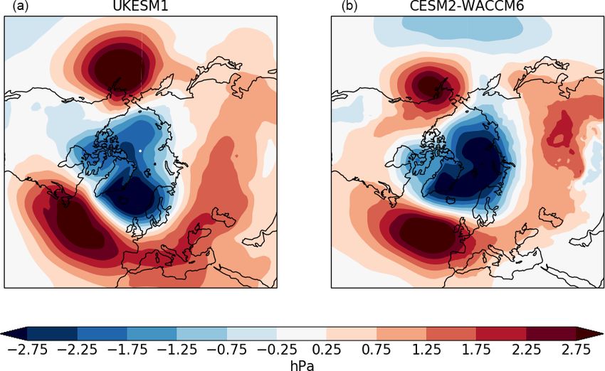
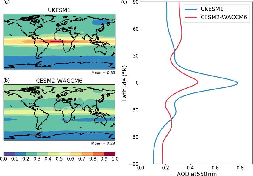
A. Jones et al.: North Atlantic Oscillation response in GeoMIP experiments G6solar and G6sulfur                           1291

Figure 1. Annual-mean temperature change (K) from present day (PD; 2011–2030 mean) to the end of the century (2081–2100 mean) in
the various experiments. Upper row (a, b, c) shows results from UKESM1 and lower row (d, e, f) for CESM2-WACCM6. All results are
ensemble means (three members for UKESM1, two for CESM2-WACCM6).

the period 2020–2070, and Niemeier et al. (2013) found that       geoengineered AOD in the tropical reservoir (e.g. Grant et
an injection rate of around 12 Tg of SO2 yr−1 was needed in       al., 1996) than in CESM2-WACCM6 where the transport to
their model by 2070. Niemeier and Timmreck (2015) sug-            higher latitudes is more efficient.
gested a massive 90 Tg of SO2 yr−1 would be needed by
2100 to offset the temperature change in the RCP8.5 sce-          4.3   Stratospheric ozone
nario (Riahi et al., 2011) in a model that explicitly simu-
lated the evolution of aerosol microphysics to larger sizes via   Stratospheric aerosol is widely acknowledged to reduce
condensation and coagulation as the injection rate increased.     stratospheric ozone through heterogeneous chemistry pro-
The increase in aerosol size leads to a decreased cooling effi-   cesses, particularly in polar regions (e.g. Solomon, 1999;
ciency per unit mass with increasing SO2 , owing to decreased     Tilmes et al., 2009), and has been studied in earlier Ge-
stratospheric lifetime (caused by higher aerosol terminal ve-     oMIP activities (e.g. Pitari et al., 2014). Both UKESM1 and
locities) and also less efficient cooling in the shortwave part   CESM2-WACCM6 include detailed stratospheric chemistry
of the spectrum along with a stronger counterbalancing im-        and are capable of modelling the impact of stratospheric
pact on terrestrial radiation (Niemeier and Timmreck, 2015).      aerosol on stratospheric ozone (Morgenstern et al., 2009;
Both UKESM1 and CESM2-WACCM6 include these micro-                 Mills et al., 2017). The impact of SAI on stratospheric ozone
physical mechanisms, so the injection rates used here are by      concentrations is shown in Fig. 3.
no means exceptional in SAI geoengineering studies.                  The SAI-induced changes in ozone concentration between
   The resulting anomalies in annual-mean aerosol optical         G6solar and G6sulfur are consistent with the distributions
depth (AOD, determined at 550 nm) for 2081–2100 are 0.33          of aerosol in the two models. UKESM1, with its higher
for UKESM1 and 0.28 for CESM2-WACCM6; their geo-                  concentration of aerosol in the tropical reservoir, shows a
graphic distributions are shown in Fig. 2.                        greater tropical ozone change, with the maximum reduction
   By 2081–2100 the AOD needed to reduce the SSP5-                centred around 20–30 hPa (∼ 24–27 km) for both models.
8.5 temperature levels to those of SSP2-4.5 is some 18 %          These changes are consistent with the findings of Tilmes et
greater for UKESM1 than for CESM2-WACCM6, although                al. (2018) and are a combination of chemical and transport
the amount of cooling produced in the two models is very          changes. The reduction in ozone concentrations in the trop-
similar (−2.47 K for UKESM1 and −2.33 K for CESM2-                ics around 20–30 hPa is the result of an increase in vertical
WACCM6). This can be attributed to the different SO2 in-          advection, while the increase in ozone above this is a result
jection strategies and to different transport strengths from      of a decreased rate of catalytic NOx ozone loss (see Tilmes
the tropics to the poles in the Brewer–Dobson circulation         et al., 2018, for more details).
of the stratosphere. In UKESM1 there is considerably more

https://doi.org/10.5194/acp-21-1287-2021                                           Atmos. Chem. Phys., 21, 1287–1304, 2021
1292                 A. Jones et al.: North Atlantic Oscillation response in GeoMIP experiments G6solar and G6sulfur

Figure 2. The distribution of the 2081–2100 mean anomaly in annual mean AOD at 550 nm (dimensionless) due to stratospheric SO2
injection for UKESM1 (a), CESM2-WACCM6 (b) and zonal means for both models (c). The anomaly is calculated from the difference
between G6sulfur and G6solar.

Figure 3. The difference in 2081–2100 annual-mean ozone concentrations (µg m−3 ) diagnosed from {G6sulfur minus G6solar} for
UKESM1 (a) and CESM2-WACCM6 (b).

4.4    Stratospheric temperature                                 is injected and the resulting stratospheric AOD is greatest
                                                                 (Fig. 2). Differences between the models’ aerosol and radia-
Perturbations to stratospheric temperatures are a key mech-      tion schemes mean that CESM2-WACCM6 has slightly more
anism implicated in observed and modelled changes in the         warming in the tropical stratosphere despite having some-
Northern Hemisphere wintertime NAO subsequent to strato-         what lower AOD compared with UKESM1. Although strato-
spheric aerosol injection from volcanoes (e.g. Stenchikov        spheric sulfate is primarily a scattering aerosol in the solar
et al., 2002; Lorenz and Hartmann, 2003; Shindell et al.,        part of the spectrum, the small amount of absorption of so-
2004). The annual-mean and the Northern Hemisphere win-          lar radiation by stratospheric aerosols in the near-infrared,
tertime (December–February) stratospheric temperature per-       together with absorption of terrestrial longwave radiation,
turbations are shown in Fig. 4.                                  causes the stratospheric heating (e.g. Stenchikov et al., 1998;
   For both models, the peak in the annual-mean tempera-         Jones et al., 2016b). Perturbations to stratospheric tempera-
ture perturbation is in the tropics, which is where the SO2

Atmos. Chem. Phys., 21, 1287–1304, 2021                                           https://doi.org/10.5194/acp-21-1287-2021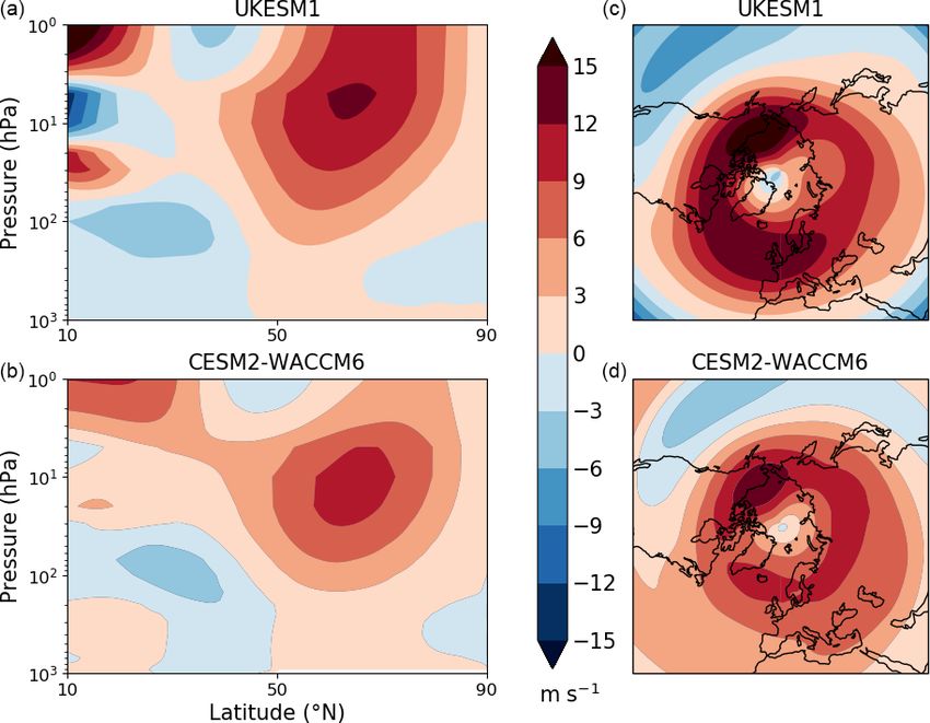
A. Jones et al.: North Atlantic Oscillation response in GeoMIP experiments G6solar and G6sulfur                               1293

Figure 4. The difference in zonal mean temperature (K) diagnosed from {G6sulfur minus G6solar}; panels (a) and (c) show results from
UKESM1 and panels (b) and (d) from CESM2-WACCM6. Panels (a) and (b) show global annual-mean results from 2081–2100; panels (c)
and (d) show Northern Hemisphere winter (December–February) means over the same period.

tures in the tropics due to less ultraviolet absorption from the    4.5.2    Tropospheric winds
reduction of stratospheric ozone (Fig. 3) play a more minor
role. The right-hand panels of Fig. 4 show that the impact of       Figure 5 shows the propagation of this enhanced westerly
solar absorption in the stratosphere cannot be effective dur-       flow to lower levels in the troposphere and to the surface,
ing the polar night. This, along with a reduced flux of ter-        with both models suggesting an increased westerly flow
restrial radiation due to low wintertime temperatures, means        north of around 50◦ N. Figure 6 shows the Northern Hemi-
that stratospheric heating from the aerosol is only present at      sphere wintertime zonal mean wind perturbation at 850 hPa
latitudes south of the Arctic Circle (Shindell et al., 2004).       induced by SAI for both models.
The cooling at high latitudes during Northern Hemisphere               As with the stratospheric winds, both models show similar
winter is consistent with a strengthening of the polar vortex       behaviour. Both show enhanced 850 hPa winds particularly
during this period.                                                 over the northern Atlantic between the southern tip of Green-
                                                                    land and the UK. This increased westerly flow penetrates into
4.5     Wind speed                                                  northern Eurasia, indicating that zonal flow is enhanced and
                                                                    shows a strong similarity to the pattern of wind speed pertur-
4.5.1    Stratospheric winds                                        bation identified in reanalysis data when the polar vortex is
                                                                    strong (e.g. Graf and Walter, 2005).
The effect that the aerosol-induced stratospheric temperature
perturbation has on the zonal mean wind speed during North-
                                                                    4.6     Mean sea-level pressure and NAO index
ern Hemisphere winter is shown in Fig. 5.
   As in Shindell et al. (2001, their Plate 5), the left-hand
                                                                    As noted in Sect. 1, the NAO may be quantified in terms
panels in Fig. 5 show that in both UKESM1 and CESM2-
                                                                    of the pressure difference between Iceland and the Azores.
WACCM6 a strong stratospheric zonal mean wind anomaly
                                                                    Here we use December–February mean sea-level pressure
develops at around 10 hPa at 60–70◦ N with an increase of
                                                                    (MSLP) from the nearest model grid cell to Stykkishól-
more than 12 m s−1 for UKESM1 and 9 m s−1 for CESM2-
                                                                    mur, Iceland (65◦ 050 N, 22◦ 440 W), and Ponta Delgada in the
WACCM6, thereby enhancing the strength of the polar vor-
                                                                    Azores (37◦ 440 N, 25◦ 410 W). We also construct an NAO in-
tex. The maximum increase in the zonal wind at this level
                                                                    dex by removing the long-term mean from the time series
is centred over Alaska in both models (right-hand panels in
                                                                    of each location’s MSLP, normalizing the resulting anoma-
Fig. 5).
                                                                    lies by their standard deviation and then taking the differ-
                                                                    ence between the normalized anomalies (e.g. Hurrell, 1995;
                                                                    Rodwell et al., 1999). A positive NAO index indicates when

https://doi.org/10.5194/acp-21-1287-2021                                             Atmos. Chem. Phys., 21, 1287–1304, 2021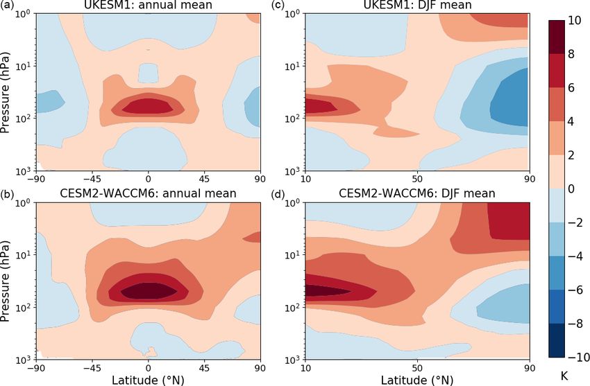
1294                    A. Jones et al.: North Atlantic Oscillation response in GeoMIP experiments G6solar and G6sulfur

Figure 5. The perturbation to mean December–February zonal wind speed over 2081–2100 (m s−1 ) caused by SAI, diagnosed from {G6sulfur
minus G6solar}. Panels (a) and (b) show the change in Northern Hemisphere zonal wind, with positive values indicating a westerly pertur-
bation and negative values an easterly one. Panels (c) and (d) show the spatial distribution of this change at 10 hPa which is the level of
maximum perturbation. Panels (a) and (c) show results from UKESM1, panels (b) and (d) those from CESM2-WACCM6.

Figure 6. The distribution of the 2081–2100 mean December–February zonal wind speed perturbation due to SAI at 850 hPa (m s−1 ) for
UKESM1 (a) and CESM2-WACCM6 (b). Positive values represent a westerly perturbation and negative values an easterly perturbation;
white areas indicate regions where the surface elevation is higher than the mean 850 hPa pressure level.

Atmos. Chem. Phys., 21, 1287–1304, 2021                                                    https://doi.org/10.5194/acp-21-1287-2021
A. Jones et al.: North Atlantic Oscillation response in GeoMIP experiments G6solar and G6sulfur 1295
the pressure difference between the two stations is greater peratures by looking at the difference between G6sulfur and
than normal, and a negative phase indicates when the pres- G6solar during the Northern Hemisphere wintertime with a
sure difference is less than normal. The perturbation to the focus on the continental scale. To put these changes in con-
mean Northern Hemisphere winter surface pressure patterns text, by experimental design the temperature changes in all
from SAI is shown in Fig. 7. experiments compared with present day (PD) show the ex-
Both models show similar large-scale perturbations to pected warming of climate commensurate with the SSP2-
MSLP with a vast swath of high-pressure anomalies centred 4.5 scenario (annual-mean changes from PD to 2081–2100
over the Atlantic Ocean at around 50◦ N and to the south of shown in Fig. 1). The purpose of examining regional changes
Alaska. The patterns of increased MSLP are broadly simi- in temperature is to emphasize that despite the inter-model
lar over Eurasia but are subtly different over the continen- similarity of response of many dynamical features associated
tal USA. A strong area of anomalous low pressure is evi- with the NAO, there are considerable inter-model differences
dent towards the pole in both models, and the strongest pres- in the resulting regional temperatures in some areas.
sure gradient anomaly is over the northern Atlantic. This Both models indicate that SAI induces broad-scale pat-
area of strong baroclinicity is associated with the strength- terns of temperature perturbation over Eurasia during North-
ening zonal flow shown in Fig. 6. Over the period 2081– ern Hemisphere winter resembling those associated with a
2100, SAI causes the NAO index in UKESM1 to change positive phase of the NAO observed subsequent to large trop-
from −0.36 in G6solar to +0.73 in G6sulfur. This corre- ical volcanic eruptions (Shindell et al., 2004), i.e. a warming
sponds to the Azores to Iceland pressure difference increas- to the north and a cooling to the south of ∼ 50◦ N (Fig. 8).
ing from 16.4 hPa (G6solar) to 22.3 hPa (G6sulfur), indicat- Explosive volcanic eruptions provide a very useful, albeit im-
ing a strengthening of the NAO of around +6 hPa, which perfect, analogue for stratospheric aerosol injection geoengi-
is significant as the standard error due to natural variabil- neering (Robock et al., 2013). The facts that similar tempera-
ity is around 1 hPa. In CESM2-WACCM6, the NAO index ture patterns are observed following explosive volcanic erup-
increases from −0.34 (G6solar) to +0.77 (G6sulfur), cor- tions and that the proposed mechanisms for impacting the
responding to a change in pressure difference of 21.3 to strength of the NAO are identical for volcanic and geoengi-
25.9 hPa, indicating a strengthening of around 4.5 hPa, which neering cases suggest that the inducing of positive phases of
is again significant compared with natural variability. the NAO under SAI geoengineering is a relatively robust con-
Before concluding that such impacts on the Northern clusion.
Hemisphere wintertime NAO are an important difference be- While there are similarities in the broad-scale hemispheric
tween end-of-century climates produced by the two different pattern of temperature perturbations, over continental North
forms of SRM geoengineering, we need to assess if there are America the models suggest rather different regional tem-
any systematic changes in the NAO over the course of the perature responses. In UKESM1 the induced positive phase
21st century in the absence of geoengineering. As noted by of the NAO from SAI leads to a warming of the eastern
Deser et al. (2017), some studies project a slight positive shift side of the continent as observed (Shindell et al., 2004)
in the probability distribution of the NAO phase by the end of as well as over the north-western Atlantic, while CESM2-
the 21st century. As G6solar and G6sulfur track the temper- WACCM6 suggests a general cooling across the continent
ature evolution of the SSP2-4.5 scenario, we compare 2081– with only the warm anomaly over the North Atlantic be-
2100 means from each model’s CMIP6 ssp245 simulation ing evident. This cooling in CESM2-WACCM6 is consis-
with present day (PD, 2011–2030) means constructed from tent with the high-pressure anomaly across the whole con-
each model’s CMIP6 historical and ssp245 experiments. In tinent in this model (Fig. 7), which would enhance advec-
UKESM1 the change in Azores-to-Iceland pressure differ- tion of cold air from higher latitudes. In contrast, UKESM1
ence between PD and 2081–2100 in SSP2-4.5 is 17.6 to has a low-pressure anomaly over much of continental North
17.7 hPa (NAO index essentially unchanged at +0.19), and America, which would have the opposite tendency. It is gen-
in CESM2-WACCM6 the corresponding values are 21.3 to erally accepted that Northern Hemisphere wintertime con-
19.8 hPa (NAO index change −0.26 to −0.63). It is therefore ditions over the eastern USA are anomalously warm during
clear that the impact of SAI geoengineering on the Northern the positive phase of the NAO (e.g. http://climate.ncsu.edu/
Hemisphere wintertime NAO dominates over any effects due images/edu/NAO2.jpg, last access: 22 January 2021) which
to global warming over this period. perhaps indicates that UKESM1 may reproduce this phase of
the NAO with greater fidelity. In contrast, however, CESM2-
4.7 Regional mid-latitude temperature WACCM6 seems to better represent the cooling observed at
high latitudes over North America following large volcanic
We have seen that both models simulate the impact of SAI eruptions. Significant cooling is also observed over northern
by inducing a positive phase of the NAO with both models Africa following such eruptions with cold anomalies extend-
showing similar patterns of response in stratospheric heat- ing to around 10◦ N (Shindell et al., 2004). Both models show
ing, stratospheric and tropospheric winds, and MSLP. We cool anomalies in this region but they extend further south in
now briefly examine the impact of SAI on near-surface tem-
https://doi.org/10.5194/acp-21-1287-2021 Atmos. Chem. Phys., 21, 1287–1304, 20211296 A. Jones et al.: North Atlantic Oscillation response in GeoMIP experiments G6solar and G6sulfur
Figure 7. The change induced by SAI in 2081–2100 mean December–February MSLP (hPa) for UKESM1 (a) and CESM2-WACCM6 (b)
diagnosed from {G6sulfur minus G6solar}.
Figure 8. The perturbation to 2081–2100 mean December–February near-surface air temperature (K) induced by SAI diagnosed from
{G6sulfur minus G6solar} for UKESM1 (a) and CESM2-WACCM6 (b). The area plotted is chosen to replicate that presented by Shindell et
al. (2004, their Fig. 2).
UKESM1 compared with CESM2-WACCM6, suggesting a areas of the UK and concluded that precipitation and stream-
somewhat weaker response to SAI in the latter model. flow is considerably enhanced during positive phases of the
NAO. On larger scales, López-Moreno et al. (2008) and
4.8 Regional mid-latitude precipitation Casanueva et al. (2014) conclude that, during the positive
phase of the NAO, positive precipitation anomalies occur
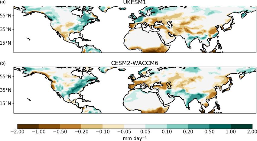
Over Europe, while the models exhibit some differences in over northern Europe while negative precipitation anomalies
the exact demarcation between increased precipitation over occur over southern Europe. Furthermore, the study of Za-
northern Europe and Scandinavia and decreased precipitation nardo et al. (2019) indicates that the NAO clearly correlates
over southern Europe (Fig. 9), the general patterns are clearly with the occurrence of catastrophic floods across Europe (and
in line with observations during positive phases of the NAO. the associated economic losses) and that over northern Eu-
For example, Fowler and Kilsby (2002) and Burt and How-
den (2013) investigated precipitation anomalies in northern
Atmos. Chem. Phys., 21, 1287–1304, 2021 https://doi.org/10.5194/acp-21-1287-2021A. Jones et al.: North Atlantic Oscillation response in GeoMIP experiments G6solar and G6sulfur 1297
rope the majority of historic winter floods occurred during a therefore evident that the idealized approach of G6solar does
positive NAO phase. not adequately represent the regional impacts on precipita-
Over North America, both models are consistent and tion over Europe.
indicate an increase in wintertime precipitation, which is Generally, the conclusions from UKESM1 presented in
again consistent with observations of wintertime precipita- Fig. 10 are supported by the results from CESM2-WACCM6
tion anomalies during the positive phase of the NAO. There (Fig. 11). The strong signal of increased precipitation in
are fewer quantitative studies of the impacts of the NAO over northern Europe evident in ssp585 is reduced in ssp245,
North America as the social and economic costs are not so G6solar and G6sulfur. G6sulfur again shows a greater re-
readily apparent as over Europe. However, an analysis by duction in precipitation south of about 45◦ N when com-
Durkee et al. (2008) indicates positive anomalies of rain over pared with G6solar. The implications of these findings are
south-eastern states and positive anomalies of snowfall over discussed in more detail in the following section.
north-eastern states during positive phases of the NAO.
4.9 Contextualizing in terms of changes compared with 5 Discussion and Conclusions
present-day precipitation
Using data from two Earth system models, we have com-
We have shown that the SAI-induced response of the NAO pared the final 20 years from two numerical experiments
and the associated impacts on precipitation are relatively well which employ different representations of geoengineering
understood and reasonably consistent between the two mod- in a scenario where the amount of cooling generated is the
els. As in earlier modelling and observational studies, the im- same. The G6solar experiment achieves the required cooling
pact is particularly marked over Europe, with northern Eu- by the highly idealized method of reducing the solar con-
rope experiencing enhanced precipitation and southern Eu- stant over the course of the 21st century, while the G6sulfur
rope reduced precipitation. We therefore focus our attention experiment achieves the same degree of cooling by inject-
on the magnitude of the SAI-induced feedbacks on precip- ing increasing amounts of SO2 into the tropical lower strato-
itation from the positive NAO anomaly compared with the sphere (SAI geoengineering). Comparing the results from
temperature- and circulation-induced feedbacks on precipita- the two experiments should help cast light on geoengineer-
tion from global warming over the European area. We do this ing impacts which only become evident when the method of
by comparing end-of-century (2081–2100) precipitation in geoengineering is represented with some fidelity.
UKESM1 and CESM2-WACCM6 with that from the present Although both models’ SAI simulations are successful in
day (PD, 2011–2030) for the ssp585, ssp245, G6solar and cooling from SSP5-8.5 to SSP2-4.5 levels, the resulting per-
G6sulfur simulations (Fig. 10 for UKESM1 and Fig. 11 for turbations to the AOD distribution are by no means identi-
CESM2-WACCM6). cal. Differences far larger than these have been reported in
As expected, Fig. 10 shows that the precipitation changes earlier coordinated GeoMIP simulations. Pitari et al. (2014,
in 2081–2100 compared with PD are significantly less in their Fig. 3d) indicate that some models (e.g. GEOSCCM)
ssp245 than in ssp585. North of 50◦ N there are many areas perform similarly to UKESM1 in maintaining a peak AOD
in ssp585 that experience a change in precipitation exceed- of 3 times that at mid-latitudes in the tropical reservoir, while
ing +0.5 mm d−1 , while south of 45◦ N areas tend to be drier other models (e.g. GISS-E2-R) show almost the opposite be-
than in PD; these patterns are consistent with the patterns haviour with a peak AOD twice that in the tropical reservoir
of precipitation and runoff changes in multi-model climate at mid-latitudes. Pitari et al. (2014) caution that aspects of
change simulation assessments (Kirtman et al., 2013; Guer- the performance of these two models are hampered by the
reiro et al., 2018). When comparing the future precipitation lack of explicit treatment of heterogeneous chemistry (GISS-
response in G6sulfur to that in ssp245, it is evident that the E2-R) and the lack of impact of the stratospheric aerosol on
precipitation anomaly pattern from the NAO-induced feed- photolysis rates (GEOSCCM); these caveats do not apply to
back (Fig. 9) acts to reinforce the temperature-induced pre- the UKESM1 and CESM2-WACCM6 models, which include
cipitation feedback. Compared with ssp245, the precipitation these processes.
anomaly in G6sulfur is more positive in northern Europe and The results from both models indicate that a key impact of
more negative in southern Europe, with a negative anomaly tropical SAI geoengineering is the generation of a persistent
that encompasses the area all around the Black Sea. When positive phase of the NAO during Northern Hemisphere win-
comparing the future precipitation response in G6sulfur with tertime. The intensification of the stratospheric jet produces
G6solar, it is evident that while the precipitation increases an increase in surface zonal winds over the North Atlantic,
north of around 50◦ N show some consistency between the leading to a warming of the Eurasian continent northwards
two, there is no such agreement further south. Over Iberia, of about 50◦ N and the associated risks of flooding in north-
Italy, the Balkans, Greece, Turkey, Ukraine and southern ern European regions (e.g. Scaife et al., 2008). The mecha-
Russia the precipitation anomalies show a wintertime precip- nism for generating these anomalies appears to be the same
itation decrease in G6sulfur but an increase in G6solar. It is as that observed following large explosive volcanic eruptions
https://doi.org/10.5194/acp-21-1287-2021 Atmos. Chem. Phys., 21, 1287–1304, 20211298 A. Jones et al.: North Atlantic Oscillation response in GeoMIP experiments G6solar and G6sulfur
Figure 9. The perturbation to 2081–2100 mean December–February land precipitation rate (mm d−1 ) induced by SAI diagnosed from
{G6sulfur minus G6solar} for UKESM1 (a) and CESM2-WACCM6 (b).
Figure 10. Changes in mean December–February land precipitation rate (mm d−1 ) between present day (PD, 2011–2030) and 2081–2100
in experiments ssp245, ssp585, G6solar and G6sulfur in UKESM1. PD means are constructed in the same manner as in Fig. 1.
in the tropics. This is consistent with the form of SAI sim- G6solar and G6sulfur provide an example relating to a crit-
ulated in G6sulfur being essentially equivalent to a continu- ical argument that has been circulating in the geoengineer-
ous, large volcanic eruption in the tropics and indicates that ing community for over a decade: that of winners and losers
the response to any putative, continuous large-scale SO2 in- (e.g. Irvine et al., 2010; Kravitz et al., 2014). While few
jection is likely to be the same as that which has been sug- would argue against the benefits of ameliorating the changes
gested to follow large sporadic eruptions. in wintertime precipitation under SSP5-8.5 by following the
In terms of impacts, the end-of-century (2081–2100) Eu- SSP2-4.5 scenario (Figs. 10 and 11), the situation is differ-
ropean wintertime precipitation anomalies in ssp585, ssp245, ent when examining the changes seen in G6sulfur. For exam-
Atmos. Chem. Phys., 21, 1287–1304, 2021 https://doi.org/10.5194/acp-21-1287-2021A. Jones et al.: North Atlantic Oscillation response in GeoMIP experiments G6solar and G6sulfur 1299
Figure 11. Same as Fig. 10 but for CESM2-WACCM6.
ple, when taking the results from CESM2-WACCM6 at face system but also deal with governance, unknowns, ethics and
value, one might argue that the impacts of the wintertime aesthetics. Furthermore, the technology to inject sulfur into
drying of vast swathes of the European continent surround- the stratosphere does not currently exist. Before any decision
ing the Mediterranean Sea (Fig. 11) might be more damaging by society to start climate intervention, much more work is
in terms of their impact on biodiversity, ecology and peoples’ needed to quantify all these potential benefits and risks. In
lives than the impact of increased flood risk in northern Eu- the meantime, even if some climate intervention is used for
rope under even the extreme SSP5-8.5 scenario. Of course, a time, there remains a great deal of work on mitigation and
here we are limited to analysing the results from just two adaptation to address the threat of global warming.
Earth system models which take no account of trying to tai-
lor the injection strategy to minimize residual climate im-
pacts (e.g. MacMartin et al., 2013), and studies have shown Code availability. Due to intellectual property rights restrictions,
that SAI can ameliorate many regional impacts of climate we cannot provide either the source code or documentation
change (e.g. Jones et al., 2018). Nevertheless, the impact of papers for the Met Office Unified Model. The UM is avail-
the SAI-induced effects on the NAO indicate the need for able for use under licence – for further information on how
to apply for a licence, see http://www.metoffice.gov.uk/research/
detailed modelling of geoengineering processes when con-
modelling-systems/unified-model (last access: 23 July 2020). Pre-
sidering the potential regional impacts of such actions. Stud- vious and current Community Earth System Model (CESM) ver-
ies which have investigated the issue of geoengineering win- sions are freely available at http://www.cesm.ucar.edu/models/
ners and losers have generally studied results from ideal- cesm2 (last access: 23 July 2020).
ized solar reduction approaches to geoengineering and there-
fore may have missed some of the effects shown here. The
differences in regional response over the continental USA Data availability. The simulation data used in this study are
and Africa (e.g. Fig. 8) demonstrate that inter-model uncer- archived on the Earth System Grid Federation (ESGF) (https://
tainty remains and indicate that more models need to perform esgf-node.llnl.gov/projects/cmip6, last access: 23 July 2020). The
these simulations before any conclusions regarding potential model source IDs are UKESM1-0-LL for UKESM1 and CESM2-
continental-scale climate change under SRM are drawn. WACCM for CESM2-WACCM6.
In addition to the potential climate impacts from SAI
shown here, such intervention would produce many other
benefits and risks (e.g. Robock, 2020). Some of these ad- Author contributions. AJ and JMH led the analysis and wrote the
ditional risks are related not only to the physical climate article with contributions from ACJ, ST, BK and AR. The UKESM1
https://doi.org/10.5194/acp-21-1287-2021 Atmos. Chem. Phys., 21, 1287–1304, 20211300 A. Jones et al.: North Atlantic Oscillation response in GeoMIP experiments G6solar and G6sulfur
and CESM2-WACCM6 simulations were carried out by AJ and ST, and UKESM1, J. Adv. Model. Earth Sy., 11, 4377–4394,
respectively. BK was central in coordinating the GeoMIP6 activity. https://doi.org/10.1029/2019MS001866, 2019.
Archibald, A. T., O’Connor, F. M., Abraham, N. L., Archer-
Nicholls, S., Chipperfield, M. P., Dalvi, M., Folberth, G. A., Den-
Competing interests. The authors declare that they have no conflict nison, F., Dhomse, S. S., Griffiths, P. T., Hardacre, C., Hewitt, A.
of interest. J., Hill, R. S., Johnson, C. E., Keeble, J., Köhler, M. O., Morgen-
stern, O., Mulcahy, J. P., Ordóñez, C., Pope, R. J., Rumbold, S.
T., Russo, M. R., Savage, N. H., Sellar, A., Stringer, M., Turnock,
Acknowledgements. Andy Jones would like to thank the Met Office S. T., Wild, O., and Zeng, G.: Description and evaluation of
team responsible for the managecmip software which greatly sim- the UKCA stratosphere–troposphere chemistry scheme (Strat-
plified the work involved. Andy Jones and Jim M. Haywood were Trop vn 1.0) implemented in UKESM1, Geosci. Model Dev., 13,
supported by the Met Office Hadley Centre Climate Programme 1223–1266, https://doi.org/10.5194/gmd-13-1223-2020, 2020.
funded by the UK Government Department for Business, Energy Best, M. J., Pryor, M., Clark, D. B., Rooney, G. G., Essery, R. L.
and Industrial Strategy (BEIS) and the UK Government Depart- H., Ménard, C. B., Edwards, J. M., Hendry, M. A., Porson, A.,
ment for Environment, Food and Rural Affairs (Defra). The CESM Gedney, N., Mercado, L. M., Sitch, S., Blyth, E., Boucher, O.,
project is supported primarily by the US National Science Foun- Cox, P. M., Grimmond, C. S. B., and Harding, R. J.: The Joint
dation (NSF). Some of the material is based upon work supported UK Land Environment Simulator (JULES), model description –
by the National Center for Atmospheric Research (NCAR) which Part 1: Energy and water fluxes, Geosci. Model Dev., 4, 677–699,
is a major facility sponsored by the NSF. Computing and data stor- https://doi.org/10.5194/gmd-4-677-2011, 2011.
age resources for CESM, including the Cheyenne supercomputer Burt, T. P. and Howden, N. J. K.: North Atlantic Os-
(https://doi.org/10.5065/D6RX99HX), were provided by the Com- cillation amplifies orographic precipitation and river flow
putational and Information Systems Laboratory (CISL) at NCAR. in upland Britain, Water Resour. Res., 49, 3504–3515,
Support for Ben Kravitz was provided in part by the NSF, the In- https://doi.org/10.1002/wrcr.20297, 2013.
diana University Environmental Resilience Institute and the Pre- Casanueva, A., Rodríguez-Puebla, C., Frías, M. D., and González-
pared for Environmental Change Grand Challenge initiative. The Reviriego, N.: Variability of extreme precipitation over Eu-
Pacific Northwest National Laboratory is operated for the US De- rope and its relationships with teleconnection patterns, Hydrol.
partment of Energy by Battelle Memorial Institute. Alan Robock Earth Syst. Sci., 18, 709–725, https://doi.org/10.5194/hess-18-
is supported by the NSF. We acknowledge the World Climate Re- 709-2014, 2014.
search Programme which, through its Working Group on Coupled Da-Allada, C. Y., Baloïtcha, E., Alamou, E. A., Awo, F. M.,
Modelling, coordinated and promoted CMIP. We thank the climate Bonou, F., Pomalegni, Y., Biao, E. I., Obada, E., Zandagba,
modelling groups for producing and making available their model J. E., Tilmes, S., and Irvine, P. J.: Changes in West
output, ESGF for archiving the data and providing access, and the African summer monsoon precipitation under stratospheric
multiple funding agencies that support CMIP6 and ESGF. We also aerosol geoengineering, Earths Future, 8, e2020EF001595,
thank all participants of the Geoengineering Model Intercomparison https://doi.org/10.1029/2020EF001595, 2020.
Project and their model development teams. Danabasoglu, G., Bates, S. C., Briegleb, B. P., Jayne, S. R.,
Jochum, M., Large, W. G., Peacock, S., and Yeager, S. G.:
The CCSM4 Ocean Component, J. Climate, 25, 1361–1389,
https://doi.org/10.1175/JCLI-D-11-00091.1, 2012.
Financial support. This research has been supported by the De-
Danabasoglu, G., Lamarque, J.-F., Bacmeister, J., Bailey, D. A.,
partment for Business, Energy and Industrial Strategy, UK Gov-
DuVivier, A. K., Edwards, J., Emmons, L. K., Fasullo, J., Gar-
ernment, the Department for Environment, Food and Rural Affairs,
cia, R., Gettelman, A., Hannay, C., Holland, M. M., Large,
UK Government, the US National Science Foundation under coop-
W. G., Lauritzen, P. H., Lawrence, D. M., Lenaerts, J. T.
erative agreement 1852977, agreement CBET-1931641 and grant
M., Lindsay, K., Lipscomb, W. H., Mills, M. J., Neale, R.,
AGS-2017113, the US National Center for Atmospheric Research,
Oleson, K. W., Otto-Bliesner, B., Phillips, A. S., Tilmes, S.,
the Indiana University Environmental Resilience Institute and the
van Kampenhout, L., Vertenstein, M., Bertini, A., Dennis, J,
Prepared for Environmental Change Grand Challenge initiative.
Deser, C., Fischer, C., Fox-Kemper, B., Kay, J. E., Kinnison,
D., Kushner, P. J., Larson, V. E., Long, M. C., Mickelson, S.,
Moore, J. K., Nienhouse, E., Polvani, L., Rasch, P. J., and
Review statement. This paper was edited by Peter Haynes and re- Strand, W. G.: The Community Earth System Model Version
viewed by two anonymous referees. 2 (CESM2), J. Adv. Model. Earth Sy., 12, e2019MS001916,
https://doi.org/10.1029/2019MS001916, 2020.
Deser, C., Hurrell, J. W., and Phillips, A. S.: The role of the North
Atlantic Oscillation in European climate projections, Clim. Dy-
nam., 49, 3141–3157, https://doi.org/10.1007/s00382-016-3502-
References z, 2017.
Dhomse, S. S., Emmerson, K. M., Mann, G. W., Bellouin, N.,
Andrews, T., Andrews, M. B., Bodas-Salcedo, A., Jones, G. Carslaw, K. S., Chipperfield, M. P., Hommel, R., Abraham,
S., Kuhlbrodt, T., Manners, J., Menary, M. B., Ridley, J., N. L., Telford, P., Braesicke, P., Dalvi, M., Johnson, C. E.,
Ringer, M. A., Sellar, A. A., and Senior, C. A.: Forc- O’Connor, F., Morgenstern, O., Pyle, J. A., Deshler, T., Za-
ings, feedbacks, and climate sensitivity in HadGEM3-GC3.1
Atmos. Chem. Phys., 21, 1287–1304, 2021 https://doi.org/10.5194/acp-21-1287-2021You can also read