Numerical simulation of meteorological hazards on motorway bridges
←
→
Page content transcription
If your browser does not render page correctly, please read the page content below
B      Meteorol. Z. (Contrib. Atm. Sci.), PrePub DOI 10.1127/metz/2020/1040
       © 2020 The authors
                                                                                                                    Short Contributions

Numerical simulation of meteorological hazards on motorway
bridges
Günter Gross∗

Institut für Meteorologie und Klimatologie, Universität Hannover, Germany
(Manuscript received April 30, 2020; in revised form July 1, 2020; accepted July 1, 2020)

             Abstract
             A one-dimensional boundary layer model was combined with a routine to calculate surface temperatures
             on road bridges. Forced by reanalysis data for the year 2016, simulations were performed for two bridges
             80 and 130 m in height, respectively. The results for each hour of the year were compared with on-site
             observations. In addition to the annual variation in general, temperature extremes captured by the model
             were quite reasonable. Although hourly wind speeds above the bridge were calculated less perfectly, the few
             cases of simulated and observed maximum mean winds were in good agreement.
             Keywords: boundary layer model, bridge, road surface temperature, wind on bridges

1 Introduction                                                                 than 50 °C (Beecroft et al., 2019). This situation in-
                                                                               creases the risk of accidents and leads to expensive
Bridges are vulnerable infrastructures exposed to the at-                      projects to maintain the infrastructure. Several authors
mosphere. The highest bridges can be found in China –                          have developed techniques to estimate surface temper-
Beipanjiang and Yesanguan bridges with maximum                                 atures on roads and bridges by using synoptic or cli-
heights above ground of 560 m and 470 m, respectively.                         matological surface observations. These data are used
In Germany, the Kochertalbrücke bridge has a clearance                         to calculate the temperature loads of bridge structures
height of 185 m and the recently opened Hochmosel-                             (e.g., Fouad, 1998; Lichte, 2004) or forecast short-
brücke bridge is 158 m high. Each bridge reaches re-                           term weather and road surface conditions (e.g., Raatz,
markable heights, but each one is located in com-                              1996; Jacobs and Raatz, 1996; Kangas et al., 2015).
pletely different meteorological environments than sur-                        Wistuba and Walther (2013) used the output of a
face roads.                                                                    regional climate model to force their road temperature
    Weather plays an important role in highway meteo-                          model for a period of 30 years.
rology with respect to issues related to driver safety, de-                        In the lower part of the atmosphere, wind speed
terioration of highway infrastructure, and operation and                       increases with height. Therefore, on a bridge several
maintenance needs (Perry and Symons, 2003). These                              hundred metres high, wind exposure of a vehicle on a
aspects are likely to become more important in the future                      bridge is greater than when moving on a surface road. In
as climate changes (Nasr et al., 2020; Willway et al.,                         addition to mean wind speed, sharp fluctuations in speed
2008).                                                                         pose a problem for vehicle stability (Kim et al., 2016).
                                                                               Wind shelters may reduce the risk but increase the force
    Different meteorological variables are related to spe-
                                                                               of the wind on the superstructure of a long-span bridge.
cific weather hazards on roads and bridges. In winter-
                                                                                   In this study, a one-dimensional single column
time, with surface temperatures below freezing, road
                                                                               boundary layer model was combined with a bridge
traffic is affected by hoar frost and ice. Dangerous situa-
                                                                               model to calculate road surface temperatures and wind
tions can be found along the motorway in the form of in-
                                                                               above the bridge. Forced by the results of reanalysis
termittent freeze-thaw conditions. These dangers can be
                                                                               data, this model system was used to estimate selected
reduced by salting or de-icing with spray units (Feld-
                                                                               meteorological hazards, as discussed above, on bridges
mann et al., 2011), but these methods involve consid-
                                                                               of different heights (80 m and 130 m) for one year.
erable expenditures on manpower, equipment, and re-
                                                                               Observations of the road weather information system,
sources to maintain the highway in safe condition.
                                                                               SWIS, of the German Meteorological Service were used
    During summertime, extreme high temperatures and                           to verify the model results because such a tested tool can
long heatwaves result in thermal loading on pave-                              be used to estimate potential operational failures during
ment. Roadways become vulnerable due to softening                              a bridge’s lifetime.
and traffic-related ruts at surface temperatures even less

∗ Corresponding
                                                                               2 The model system
                author: Günter Gross, Institut für Meteorologie und Klima-
tologie, Universität Hannover, Herrenhäuser Str. 2, 30419 Hannover, Ger-       The concept behind the modelling strategy was based on
many, e-mail: gross@muk.uni-hannover.de                                        a combination between a simple meteorological model

                                                                                                                           © 2020 The authors
DOI 10.1127/metz/2020/1040                                     Gebrüder Borntraeger Science Publishers, Stuttgart, www.borntraeger-cramer.com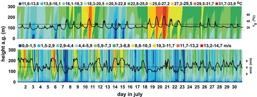
2            G. Gross: Numerical simulation of meteorological hazards on motorway bridges                Meteorol. Z. (Contrib. Atm. Sci.)
                                                                                                                    PrePub Article, 2020

Figure 1: Schematic view of the bridge structure, nomenclature and reanalysis data used (in red).

                                                                                               ⎡ 2  2 ⎤
and an embedded model to calculate temperature dis-                    ∂E    ∂      ∂E         ⎢⎢ ∂u   ∂v ⎥⎥⎥⎥       g ∂θ E 3/2
tribution within a bridge (Fig. 1). The one-dimensional                    = Km        + Km ⎢⎢⎢⎣     +       ⎥⎦ − Kh      −
                                                                       ∂t    ∂z     ∂z            ∂z   ∂z            θ ∂z      l
boundary layer model (PBL model) was forced by re-
analysis data to provide information on the meteoro-                                                                        (2.4)
logical environment of a bridge located at an arbitrary                          κz
                                                                        la =           , l∞ = 25 m, κ = 0.40                (2.5)
height. This weather information together with the spe-                      1 + κz/l∞
                                                                                √
cific structure of the bridge were used to calculate rele-             Km = ala E, a = 0.2                                  (2.6)
vant long-term information, like pavement temperatures,
to estimate selected hazards. This model concept is not               where u and v are wind components in west-east and
suitable to calculate the three-dimensional distribution              south-north directions, ug and vg are components of the
of wind speed and temperature around a bridge. How-                   larger scale synoptic wind, f is the Coriolis parameter,
ever, if a high bridge spans a wide valley, then away from            θ is the potential temperature, θg is the synoptic tem-
abutments at the beginning and the end of the bridge,                 perature, la is the mixing length, Km and Kh are eddy
i.e. mid-way through construction, the results should be              diffusivities for momentum and heat (Km = Kh = K are
reasonably horizontal homogeneous and therefore rep-                  used here) and g is acceleration due to gravity.
resentative of real conditions.                                           The effects of thermal stability on turbulent mixing
                                                                      in the boundary layer were considered by a stratification
                                                                      dependent mixing length:
2.1 The PBL model
                                                                                                    l = la /Φ                       (2.7)
In order to study longer periods for different synoptic
situations or climate scenarios, a one-dimension single               where Φ represents the local universal function which
column time-dependent boundary layer model was used                   may, according to Wippermann (1973), be expressed
(Gross, 2012; Gross, 2019). It consisted of prognos-                  as:
tic equations for the two horizontal wind components u
and v, the first law of thermodynamics written with po-                        Φ = (1 − 15z/L)−1/4 ,             z/L ≤ 0 or
tential temperature θ, and an equation for turbulence ki-                      Φ = 1 + 4.7z/L,                   z/L > 0            (2.8)
netic energy E. All turbulent fluxes were parameterised
using K-theory:                                                       where L denotes the Monin-Obukhov stability length.
                                                                         The synoptic forcing ug , vg , and θg and the bound-
∂u                  ∂    ∂u ∂ug                                       ary conditions were adopted from the high-resolution re-
   = f (v − vg ) + Km +                                      (2.1)
∂t                 ∂z    ∂z   ∂t                                      analysis system (Bollmeyer et al., 2015). The regional
∂v                    ∂   ∂v ∂vg                                      reanalysis data for the European CORDEX EUR-11 do-
   = − f (u − ug ) + Km +                                    (2.2)    main are available at a 6 km grid resolution. These val-
∂t                    ∂z   ∂z   ∂t
∂θ    ∂     ∂θ ∂θg                                                    ues were also used as boundary conditions at the upper
   = Kh +                                                    (2.3)    boundary, updated every hour, and linearly interpolated
∂t   ∂z ∂z         ∂t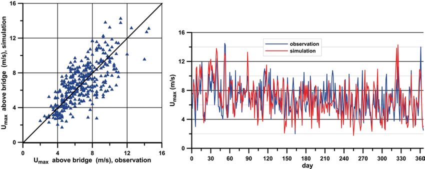
Meteorol. Z. (Contrib. Atm. Sci.)             G. Gross: Numerical simulation of meteorological hazards on motorway bridges          3
PrePub Article, 2020

Table 1: Contributions to the surface energy budget on the top and the bottom side of a bridge.

                                             Bridge surface TS                        Bridge underside TL
                          QS B                   (1 −   aB )QgS                           not considered
                                         (QgS from reanalysis data)
                           QL                        εB σT S4                                  εB σT L4
                           QgA              from the atmosphere                  from the ground under the bridge
                                           (from reanalysis data)                             εo σT o4
                                                                   −T V                                   T Atm,L −T L
                           QH             c p ρK ∂T
                                                 ∂z
                                                    = c p ρK T Atm
                                                                ΔzA
                                                                                     c p ρK ∂T
                                                                                            ∂z
                                                                                               = c p ρK       ΔzA

                           QV       function of precipitation RRg and QgS                 not considered
                           QB                   λ ∂T
                                                  ∂z
                                                     = λ T BΔz−TB S                       λ ∂T
                                                                                            ∂z
                                                                                               = λ T BΔz−TB L

in between. At the lower boundary, 2 m temperatures                         which might fail some days, the effects on the hazard
from reanalysis data were used, while zero wind condi-                      ‘high pavement temperature’ was low because extreme
tions were adopted as well as turbulence kinetic energy                     values of T S occurred during sunny days.
proportional to the simulated friction velocity squared.                        To calculate the lower boundary for air temperature
    The equations were integrated forward in time on                        above the bridge, an additional thin microlayer in which
70 grid levels in the atmosphere with a time step of                        molecular processes dominate was included at the in-
Δt = 60 s. The grid resolution was 10 m up to a height                      terface between the smooth road surface and the atmo-
of 400 m, followed by continuous expansion up to the                        sphere. Assuming that the molecular heat flux at the sur-
model height of 2000 m.                                                     face is equal to the turbulent heat flux at the top of the
                                                                            microlayer (Stull, 1988), the air temperature T V at the
2.2 The bridge model                                                        top of the viscous layer above the bridge can be calcu-
                                                                            lated as:
The bridge structure used in this study was a long-span                                               T S + cT Atm
box girder bridge made of steel or reinforced concrete.                                         TV =                             (2.9)
The bridge deck was covered with an asphalt surface                                                       1+c
course and a binder course, together 8 cm thick, which                      with c = νKΔz  V
                                                                                       L ΔzA
                                                                                             and νL = 1.5 × 10⁻⁵ m2 /s for air and a
were applied to the subbase and the bridge construction                     viscous layer depth of ΔzV = 1 mm.
(Fig. 1). The lower part of the girder consisted of a solid                    The height of the rainwater h (in mm) on the surface
construction of 20 cm thickness.                                            was calculated according to:
    As summarized in Table 1, temperatures at the bridge
surface T S and the underside of the bridge T L were de-                                              QV
                                                                                            ht+Δt = ht − Δt + RRg Δt        (2.10)
rived by a surface energy budget which included short-                                                 L
wave radiation balance QS B , longwave radiation QL ,                       with latent heat L and precipitation RRg (mm/s). The
longwave radiation from above or below QA , turbulent                       range of h is limited to h = 0 (dry surface, QV = 0)
fluxes of sensible and latent heat QH and QV , and heat                     and h = 2 mm. For larger values of h, surface run off
transfer into the underlying structure QB (e.g., Stull,                     removes the excess water.
1988). A positive sign is used for an energy gain, a neg-                      For temperatures inside the bridge material T B , the
ative sign for energy loss of the surface.                                  heat conduction equation is:
    In the equations above, aB is albedo, ε is emissiv-
ity (εB for the bridge and εo for the surface beneath                                                 ∂T B     ∂2 T B
the bridge), c p is specific heat, ρ is air density, T Atm is                                              = υB 2              (2.11)
                                                                                                       ∂t       ∂zB
simulated temperature at nearest grid level in the atmo-
sphere above and T Atm,L below the bridge at distance                       with thermal diffusivity νB . Depending on the inner
ΔzA = 10 m, λ is thermal conductivity, and T B is the                       structure of the bridge, different values for νB were
simulated internal temperature of the bridge at distance                    specified for each layer.
ΔzB = 2 cm.                                                                     Based on data published by Fouad (1998) and
    Evaporation is an important factor which determines                     Lichte (2004), the properties of the asphalt surface
the surface temperature T S . When the road surface is dry                  layer were fixed with aB = 0.2, εB = 0.9, νB =
(QV = 0), a large portion of the direct solar radiation is                  0.4 × 10⁻⁶ m2 /s and λ = 0.8 W/m/K. For steel and re-
used for heating the road’s surface. When water is avail-                   inforced concrete, values of νB = 13 × 10−6 m2 /s and
able on the road (e.g., after precipitation), a rough esti-                 νB = 0.7 × 10⁻⁶ m2 /s were used, respectively. The emis-
mate of QV = 0.3 QS B was used to calculate the turbu-                      sivity of the ground under the bridge was fixed with a
lent latent heat flux. Although this is a crude assumption                  value of εo = 0.95.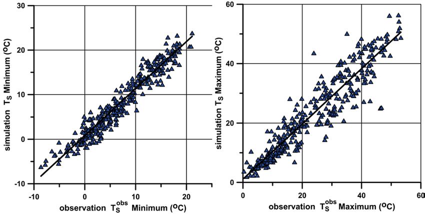
4 G. Gross: Numerical simulation of meteorological hazards on motorway bridges Meteorol. Z. (Contrib. Atm. Sci.)
PrePub Article, 2020
Figure 2: Time-height cross section for July 2016 of simulated temperature (above) and wind speed (below) at site K266 on Moseltalbrücke.
Surface temperature T S on the 130 m high bridge and wind speed at 2 m height above the bridge are enclosed in solid lines.
The temperature distribution inside the girder bridge 4 Results
was calculated at 70 levels with a time step of Δt = 60 s;
at the top and bottom, the grid resolution was 2 cm with Numerical simulations with the model system were per-
values increasing towards the inner part. formed for the full year 2016 for both bridges, whereby
results for the higher Moseltalbrücke will be discussed
3 Observations and synoptic forcing first and in more details. Wind speed and temperature for
the month July are shown as time-height cross sections
The German National Meteorological Service (DWD) in Fig. 2. A well-developed diurnal variation for tem-
collect and provides information about the surface sta- perature is evident with low nocturnal temperatures near
tus and meteorological conditions close to roads at spe- the surface and an inversion layer above. On some days,
cific sites (Glättemeldeanlagen GMAs). Every 15 min- atmospheric near surface temperatures are above 30 °C
utes, wetness and temperature of the pavement T Sobs within a well-mixed boundary layer during daytime.
are recorded as well as atmospheric temperature T 2obs m Wind speeds show periodic variations over time, with
and wind speed as a 10-min mean along the road- high values usually during the daytime. Only a few
side. Air temperature and wind are measured as stan- nights (e.g., July 14–15), did strong nocturnal winds oc-
dard at a height of 2 m and surface temperature is ob- cur which might be due to a low-level jet.
served at the outermost fast lane. Data from the year Simulated temperatures on the road surface at a
2016 for two GMAs located on high bridges were se- height of 130 m above ground are also included in Fig. 2.
lected (Koelschtzky, 2018, personell communication) During the sunny period (July 19–21), maximum tem-
to compare with the model. The Moseltalbrücke bridge peratures T S were above 50 °C. One hour mean wind
(GMA K266), located to the west of Koblenz, is a 936 m speeds at a height of 2 m above the bridge deck, the
long-span steel bridge with a superstructure height of usual measuring height of a GMA, were calculated us-
around 6 m and a maximum height of the roadways ing a log-linear law with simulated wind speeds at 10 m
above ground of 136 m. Data availability for the year above the bridge and a surface roughness length of 1 cm.
2016 was 98.5 %. For synoptic forcing, reanalysis of These values, at a height of approximately 130 m above
data in 1 hour intervals at a grid point with coordi- ground, are also included in Fig. 2 and show strong
nates (longitude/latitude) 50.359 N/7.498 E were used; variations with maximum values up to 8 m/s. Using the
however, precipitation was not available with a 1 hour temperature T V near the surface and the temperature
resolution, therefore data from the nearby synoptic sta- 10 m above the bridge T Atm , a 2 m air temperature was
tion Andernach (ID 0161) were used. For an addi- calculated in the same way.
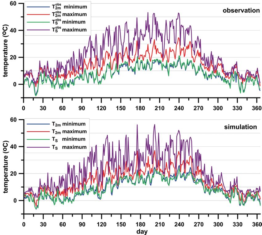
tional application, the 845 m long Haseltalbrücke bridge In Fig. 3, a comparison between the simulated and
(GMA M731) near Suhl was chosen. The maximum the observed minimum and maximum surface temper-
height above ground of this girder bridge with a super- atures and the 2 m temperatures is presented. The ob-
structure height of 5 m is 80 m. Data availability was servations at GMA K266 on the 130 m high Moseltal-
95–99 % for meteorological parameters at the roadside brücke bridge show maximum surface temperatures that
and 90 % for road surface temperatures. Reanalysis data frequently exceed 40 °C between day 120 and day 250.
from a grid point with coordinates 50.603 N/10.674 E Minimum surface temperatures were regularly below
and hourly precipitation data from the synoptic station freezing between days 1 and 120 and days 310 to 366.
Erfurt-Weimar (ID 1270) were used to specify the syn- The main features of the annual course of simulated
optic forcing. temperatures are in close agreement with the observa-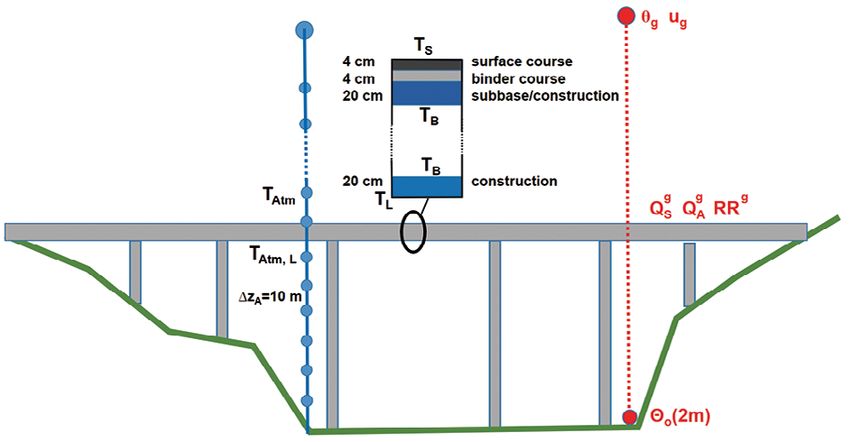
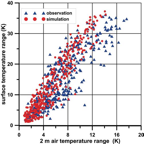
Meteorol. Z. (Contrib. Atm. Sci.)         G. Gross: Numerical simulation of meteorological hazards on motorway bridges          5
PrePub Article, 2020

Figure 3: Observed (above) and simulated (below) annual variation of daily minimum and maximum temperatures of road surface and at
2 m height above the road at site K266 on Moseltalbrücke.

tions. Only during the summer months were minimum                 Although amplitudes showed large values, simulated
road surface temperatures and nocturnal 2 m air tem-              results capture the overall picture of the observations
peratures higher than the observed values. This agree-            quite well.
ment is also evidenced by direct comparison (Fig. 4).                 High wind speeds and strong gusts can increase the
Daily maximum road surface temperatures and night-                danger to vehicles crossing a wind-exposed infrastruc-
time minimum road surface temperatures were simu-                 ture such as a high bridge. In addition to strong day-
lated in the same order as the observed values. A statisti-       to-day variations, the synoptic conditions at the selected
cal evaluation of mean absolute difference MAD and co-            sites caused higher values of mean wind speed during
efficient of determination R2 results in MAD = 1.7 K und          winter and lower values during the summer months. In
R2 = 0.93 for the night-time situation and MAD = 3.3 K            Fig. 6, the observed maximum 1 hour mean wind speed
and R2 = 0.88 for daytime respectively. Simulated and             for each day of the year 2016 at Moseltalbrücke is given
observed maximum temperatures for some days were                  together with the simulated wind speed. The numerical
well above 50 °C, while simulated road surface temper-            results follow the observations closely which is addi-
atures were below freezing on 55 days compared to an              tional evidence for comparison (Fig. 6). Although there
observed number of 61 days. Beside these mean surface             is some scatter, the simulation captures the range of the
temperature extremes, daily range between maximum                 observed wind speed (MAD = 1.4 m/s and R2 = 0.56).
and minimum temperatures were compared (Fig. 5). The                  Depending on traffic, speed, size, and load of motor
same analysis was performed for the 2 m air temper-               vehicles, wind speed might pose a danger for vehicles
ature above the bridge, estimated by a log-linear law.            crossing a long high bridge. Kim et al. (2016) estimated
6            G. Gross: Numerical simulation of meteorological hazards on motorway bridges                Meteorol. Z. (Contrib. Atm. Sci.)
                                                                                                                    PrePub Article, 2020

Figure 4: Simulated and observed daily minimum (left) and maximum (right) surface temperatures at site K266 on Moseltalbrücke.

                                                                      Table 2: Comparison of observed and simulated frequency of se-
                                                                      lected meteorological caused hazards at the Moseltalbrücke (K266)
                                                                      and the Haseltalbrücke (M731) for the year 2016.

                                                                                           observation               simulation
                                                                                          K266 M731 K266 M731 K266                  M731
                                                                      days with U > Bf 7 3       0        2      1        ugust : 16 27
                                                                      days with U > Bf 8 0       0        0      0        ugust : 2 2
                                                                      hours T S < 0 °C   420     859      363    753
                                                                      freeze-thaw change 86      125      97     190
                                                                      hours T S > 40 °C   232    108      214    102
                                                                      hours T S > 45 °C   84     31       86     30
                                                                      hours T S > 50 °C   20     4        20     6

                                                                      where σu is the standard deviation of wind speed calcu-
                                                                      lated via the turbulence kinetic energy, and the factor fg
                                                                      is typically on the order of three (Koss, 2006).
                                                                          Meteorological hazards due to temperature in win-
Figure 5: Simulated and observed diurnal ranges of the road surface
                                                                      tertime are situations with temperatures below zero and
temperature and the air temperature at 2 m height above the road at   changes in freeze-thaw conditions. In summertime, high
site K266 on Moseltalbrücke.                                          surface temperatures may cause severe damage to the
                                                                      road surface and the substructure. In Table 2, these
                                                                      hazards are summarised for the Moseltalbrücke and
critical wind speeds at a Beaufort scale of Bf 8 to Bf 9              Haseltalbrücke sites for the year 2016 for the observa-
(approximately 17–24 m/s) for sideslip and overturning                tions and the simulation.
of motor vehicles. High wind speeds may occur as a                        The numerical results are close to the observations
generally high mean wind speed U or as a sudden and                   and thus demonstrate that the model combination from
unforeseen gust event ugust . Gusts are not measured                  reanalysis data down to the bridge model is an encour-
at the GMA but may be estimated by the calculated                     aging procedure to estimate in situ meteorological con-
wind speed and turbulence information generated by the                ditions. As observed at GMA K266 and in the simula-
model. An approach commonly used in practice is given                 tion results, the 10-min mean wind speed on the bridge
by:                                                                   did not reach gale force; however, in the simulation,
                                                                      wind gusts occurred on several days with short time peak
                       ugust = U + fg σu                     (4.1)    winds exceeding Bf 8.
Meteorol. Z. (Contrib. Atm. Sci.) G. Gross: Numerical simulation of meteorological hazards on motorway bridges 7
PrePub Article, 2020
Figure 6: Annual variation of daily maximum mean wind speed at 2 m above the bridge at site K266 on Moseltalbrücke (right). Comparison
of observed and simulated 2 m daily mean wind speed maximum (left).
The number of hours below freezing were underes- road at K266. Nearly all situations in the year 2016 with
timated by the model, while a large number of freeze- T S > 40 °C were captured by the model. It is noteworthy
thaw changes were simulated. However, the numbers that the number of high surface temperatures was much
were on the same order of magnitude and differences smaller at M731 than at K266. An obvious reason for
of 10–15 % are reasonable against the background of this finding is the lower number of days with high val-
uncertainties in observations and model results. On the ues of direct solar radiation in the reanalysis data. At
other hand, surface temperatures above 40 °C were cap- the Moseltalbrücke site in the summer period of 2016,
tured well by the model, especially extreme tempera- QS exceeded 600 W/m2 for a total of 20 days, while at
tures. Haseltalbrücke, this only occurred on seven days.
Numerical simulations were performed also for the
M731 site at Haseltalbrücke in order to test the applica-
bility of the model in an alternative situation. The pro- 5 Conclusions
cedure was the same as for the Moseltalbrücke bridge.
The quality of the results was similar, so only the com- A one-dimensional boundary layer model was used
parison of the selected meteorological hazards is given to simulate the time-height variation of wind speed
in Table 2. and temperature forced by reanalysis data from the
Wind speed, in general, was lower near M731 (an- year 2016. In this atmospheric environment, a bridge
nual mean 2.1 m/s) compared to K266 (annual mean with a certain height and local atmospheric variables, to-
3.9 m/s) due to climatological conditions and lower gether with key parameter characterising the structure of
bridge height. Mean wind speeds above Bf 6 were rare in the bridge, were used to calculate surface temperatures
the observations and in the simulation; however, closer of the pavement. In addition, atmospheric wind speed
to the ground, the turbulence was greater (Stull, 1988), and temperature at a height of 2 m above the bridge deck
and consequently, the number of simulated wind gusts were estimated. The simulation results were compared
calculated by Equation (4.1) were greater as well. to observations for two long-span bridges of 80 m and
Temperatures below zero degrees at the Haseltal- 130 m height at two sites in Germany.
brücke location were more frequent than at the Moseltal- The model system introduced here is suitable to sim-
brücke location mainly because of the general climato- ulate the diurnal and annual variation in good agree-
logical situation. Night-time minimum air temperatures ment with the available observations. High surface tem-
during the winter season are typically two degrees lower peratures, where pavement becomes vulnerable through
at M731 on the Haseltalbrücke than at K266 located softening, were captured for both bridges by the model.
on the Moseltalbrücke. In combination with lower wind Minimum winter temperatures and freeze-thaw condi-
speed, this is the reason that the number of hours be- tions were simulated with slightly poorer agreement, but
low freezing, as well as the number of freeze-thaw cy- still on the same order as observed. This is not surpris-
cles, which were much higher at Haseltalbrücke than ing since the maximum temperature mainly depends on
at Moseltalbrücke. Again, the model system reproduced the magnitude of the solar radiation, while a variety of
the order of events, but with larger differences compared parameters like fog, cloud coverage, or surface wetness
to observed values at M731 than at K266. Again, the are responsible for surface temperatures a little below or
approach used in this study was successful in simulat- above the freezing point. Observed mean wind speeds
ing the occurrence of high surface temperatures on the above the bridge never exceeded 15 m/s on both bridges8 G. Gross: Numerical simulation of meteorological hazards on motorway bridges Meteorol. Z. (Contrib. Atm. Sci.)
PrePub Article, 2020
during the year. Also, in the simulation forced by re- Feldmann, M., B. Döring, J. Hellberg, M. Kuhnhenne,
analysis data, mean wind speeds never reached stormy D. Pak, 2011: Vermeidung von Glättebildung auf Brücken
conditions; however, estimated gusts were of an order durch die Nutzung von Geothermie. – Berichte der Bundes-
that was a potential danger for vehicles moving across anstalt für Straßenwesen, Heft B 87, 77 pp.
Fouad, N.A., 1998: Rechnerische Simulation der klimatisch
the bridge deck. bedingten Temperaturbeanspruchungen von Bauwerken. –
Bridge operators need information about possible Berichte aus dem Konstruktiven Ingenieurbau, Heft 28,
meteorological hazards in order to include precaution- TU Berlin.
ary measures during the planning process or to estimate Gross, G., 2012: Numerical simulation of greening effects for
the operational failures during a bridge’s lifetime. Al- idealised roofs with regional climate forcing. – Meteorol. Z.
though presented results are very encouraging, the mod- 21, 173–181.
Gross, G., 2019: On the range of boundary layer model results
els used have limitations and involve uncertainties. All depending on inaccurate input data. Meteorol. Z. 28, 225–234.
three-dimensional features concerning the bridge struc- Jacobs, W., W.E. Raatz, 1996: Forecasting road-surface tem-
ture or meteorological characteristics in a mountain en- peratures for different site characteristics. – Meteor. Appl. 3,
vironment like channeling of the air flow in valleys or 243–256.
diurnal wind systems cannot be captured by the one- Kangas, M., M. Heikinheimo, M. Hippi, 2015: RoadSurf: a
dimensional approach. If the results of regional climate modelling system for predicting road weather and road surface
models for different scenarios can be used for large scale conditions. – Meteor. Appl. 22, 544–553.
Kim, S.E., C.-H. Yoo, H.K. Kim, 2016: Vulnerability assessment
forcing, the simple model system presented her is appli- for the hazards of crosswinds when vehicles cross a bridge
cable to estimate the impact of future climate change deck. – J. Wind Eng. Ind. Aerodyn. 156, 62–71.
on the occurrence of specific meteorological hazards on Koelschtzky, W., 2018: personal communication. – DWD Of-
bridges. fenbach.
Koss, H.H., 2006: On the differences and similarities of applied
wind comfort criteria. – J. Wind Eng. 94, 781–797.
Acknowledgements Lichte, U., 2004: Klimatische Temperatureinwirkungen und
Kombinationsregeln bei Brückenbauwerken. – Dissertation,
The author would like to thank the reviewers for their Universität der Bundeswehr, München.
Nasr, A., E. Kjellström, I. Björnsson, D. Honfi,
careful reading and very useful comments, which im- O.L. Ivanov, J. Johansson, 2020: Bridges in a chang-
proved the quality of the paper significantly. The author ing climate: a study of the potential impacts of climate
would like to thank T. Lucas, Department of Meteorol- change on bridges and their possible adaptations. – Structure
ogy and Climatology, Leibniz University Hannover for Infrastructure Engineering 16, 738–749.
providing the reanalysis data. The publication of this ar- Perry, A.H., L.J. Symons, 2003: Highway Meteorology. – Tay-
ticle was funded by the Open Access Fund of the Leibniz lor & Francise-Library.
Universität Hannover. Raatz, W.E., 1996: Straßenwettervorhersage des Deutschen
Wetterdienstes im Rahmen des Straßenzustands- und Wetter-
informationssystems (SWIS). – promet 25, 1–8.
Stull, R.B., 1988: An introduction to boundary layer meteorol-
References ogy. – Kluwer Academic, 666 pp.
Willway, T., L. Baldachin, S. Reeves, M. Harding,
Beecroft, A., D. Bodin, E. van Aswegen, J. Grobler, M. McHale, M. Nunn, 2008: The effects of climate change
2019: Roads vs extreme weather: designing more re- on carriageway and footway pavement maintenance. – Tech-
silient roads. – Infrastructure Exchange, https://www nical report PPR 184, Dept. Transport, Berkshire, UK.
.infrastructure-exchange.com/post/roads-vs-extreme-weather Wippermann, F., 1973: The planetary boundary layer. – Ann.
-designing-more-resilient-roads. Meteorol. 7, 346 pp.
Bollmeyer, C., J.D. Keller, C. Ohlwein, S. Bentzien, Wistuba, M.P., A.Walther, 2013: Soll der prognostizierte Kli-
S. Crewell, P. Friederichs, A. Hense, J. Keune, mawandel für die rechnerische Dimensionierung von Asphalt-
S. Kneifel, I. Pscheidt, S. Redl, S. Steinke, 2015: To- straßen berücksichtigt werden. – Straße und Autobahn 3,
wards a high-resolution regional reanalysis for the European 140–147.
CORDEX domain. – Quart. J. Roy. Meteor. Soc. 141, 1–15.You can also read


