Numerical study of radiative non-Darcy nanofluid flow over a stretching sheet with a convective Nield conditions and energy activation
←
→
Page content transcription
If your browser does not render page correctly, please read the page content below
Nonlinear Engineering 2021; 10: 159–176

N. Vedavathi, Ghuram Dharmaiah, Kothuru Venkatadri, and Shaik Abdul Gaffar*

Numerical study of radiative non-Darcy nanofluid
flow over a stretching sheet with a convective
Nield conditions and energy activation
https://doi.org/10.1515/nleng-2021-0012
Received Dec 19, 2020; accepted Apr 14, 2021.
                                                                       1 Introduction
Abstract: Numerous industrial processes such as contin-                Nanofluids are maneuvered by suspending nanoparticles
uous metal casting and polymer extrusion in metal spin-                with average size below 100 nm in traditional heat trans-
ning, include flow and heat transfer over a stretching                 fer fluids such as ethylene glycol, oil and water. An impor-
surface. The theoretical investigation of magnetohydro-                tant role is simulated by thermal conductivity of water, oil
dynamic thermally radiative non-Darcy Nanofluid flows                  and ethylene glycol with nanoparticles in the heat transfer
through a stretching surface is presented considering also             between the heat and mass transfer medium and the heat
the influences of thermal conductivity and Arrhenius acti-             and mass transfer surface. The rise in thermal conductiv-
vation energy. Buongiorno’s two-phase Nanofluid model is               ity is substantial in improving the heat transfer behavior of
deployed in order to generate Thermophoresis and Brow-                 the fluids. High heat transfer performance is necessitated
nian motion effects [1]. By similarity transformation tech-            by several engineering applications. In several engineer-
nique, the transport equations and the respective bound-               ing and industrial applications, the thermal conductivity
ary conditions are normalized and the relevant variable                of nanofluid is not constant and it differs linearly with tem-
and concerned similarity solutions are presented to sum-               perature. Nanofluid is the combination of nanoparticles
marize the transpiration parameter. An appropriate Mat-                with water. The addition of a surfactant to a base fluid im-
lab software (Bvp4c) is used to obtain the numerical so-               proves thermal conductivity and convective heat transfer.
lutions. The graphical influence of various thermo physi-              Nanofluid technology has emerged as a modern heat trans-
cal parameters are inspected for momentum, energy and                  fer technique that is more effective. Nanofluids are used in
nanoparticle volume fraction distributions. Tables con-                solar energy applications such as heat exchanger design,
taining the Nusselt number, skin friction and Sherwood                 medical applications such as cancer therapy and safer
number are also presented and well argued. The present                 surgery by heat treatment applications. Nanofluid technol-
results are compared with the previous studies and are                 ogy can be used to create better oil and lubricants for real-
found to be well correlated and are in good agreement. The             istic applications [2]. Many scientists and engineers have
existing modelling approach in the presence of nanoparti-              been working on fluid forming for the past few decades
cles enhances the performance of thermal energy thermo-                in order to improve efficiency for various thermal appli-
plastic devices.                                                       cations. The term “nanofluid” has been proposed to ad-
                                                                       dress the new heat transfer problems by applying nan-
Keywords: Buongiorno’s two-phase Nanofluid model, Ar-
                                                                       otechnology to heat transfer [3]. Many authors have pre-
rhenius activation energy, non-Darcy, radiation, magneto-
                                                                       dicted that nanofluids would have greater convective heat
hydrodynamics, velocity slip, Biot number

                                                                       N. Vedavathi, Department of Mathematics, Koneru Lakshmaiah
                                                                       Education Foundation, Vaddeswaram, India
                                                                       Ghuram Dharmaiah, Department of Mathematics, Narasaraopeta
                                                                       Engineering College, Yellamanda, India
                                                                       Kothuru Venkatadri, Department of Mathematics, Sreenivasa Insti-
                                                                       tute of Technology and management studies, Chittoor, India
                                                                       *Corresponding Author: Shaik Abdul Gaffar, Department of In-
                                                                       formation Technology, Mathematics Section, University of Tech-
                                                                       nology and Applied Sciences, Salalah, Oman, E-mail: abdulsgaf-
                                                                       far0905@gmail.com

   Open Access. © 2021 N. Vedavathi et al., published by De Gruyter.       This work is licensed under the Creative Commons Attribu-
tion alone 4.0 License.
160 | N. Vedavathi, Numerical study of radiative non-Darcy nanofluid flow
transfer capabilities than base fluids. Heat and mass trans- fluid flows past a semi-infinite vertical porous plate us-
fer of nanofluids have integrated many practical applica- ing the explicit finite difference technique. They observed
tions of thermal and solutal stratification. Patil et al. [4] that both heat sink and thermal diffusion have a growing
investigated the unsteady mixed convection nanoliquid effect of the species concentration and the lighter parti-
flows through an exponentially stretching surface in the cles have a higher fluid concentration compared to heavier
presence of applied transverse magnetic field with realistic ones. Alam et al. [16] considered the principles of magne-
application to solar systems. Khan et al. [5] presented the tohydrodynamics and ferrohydrodynamics to examine the
entropy analysis and gyrotactic microorganisms of Buon- biomagnetic flows of blood containing gold nanoparticles
giorno’s nanofluid between two stretchable rotating disks past a stretching surface in the presence of Biot number,
using homotopy analysis. Nainaru et al. [6] studied the suction and velocity slip using the bvp4c technique. Khan
effects of heat transfer characteristics on 3D MHD flows et al. [17] presented the entropy analysis of MHD radiative
of nanofluid induced by stretching surface with thermal flows of Jeffrey fluid past an inclined surface using Keller-
radiation. They observed a rise in the fluid temperature Box technique. Vedavati et al. [18] examined the MHD con-
and velocity with a rise in variable thermal conductivity. vection flows of nanofluid past an inverted cone consid-
Shiriny et al. [7] considered the forced convection flow of ering the suction/injection effects and entropy analysis is
nanofluid in a horizontal microchannel with cross flow also presented.
injection and slip velocity on microchannel walls. They Thermal radiation is a key aspect in many engineer-
observed that an increase in velocity slip and heat trans- ing processes that take place at extreme temperatures.
fer rate by increasing the angle of injection to 94◦ . Suhail Many industrial applications involving extreme tempera-
and Siddiqui [8] presented the numerical study the natu- tures such as gas turbines, nuclear power stations and var-
ral convection flows of nanofluid within a vertical annu- ious combustion turbines for aircraft, rockets, spacecraft
lus. They discussed the simulations for various nanoparti- and aerospace engineering have stressed the effects of ra-
cle concentrations for various heat flux values. Few recent diation on convection. Radiative heat transfer is crucial
studies on nanofluid includes [9–11]. in oxidation, fossil fuel energy cycles, astrophysical flows,
Due of its universal and practical applications, the renewable energy engineering are the other applications.
convective boundary layer plays an important role in the Mumtaz et al. [19] studied the mixed convective chemically
process of heat supply to the fluid via a particle surface radiative flows of tangent hyperbolic fluid with viscous
with a restricted heat efficiency, especially in various man- dissipation in a doubly stratified medium using BVPh2
ufacturing and advanced processes that include transpi- scheme. Yusuf et al. [20] investigated the entropy analysis
ration cooling, fabric cleaning, laser pulse heating and so on radiative MHD flows of Williamson nanofluid past an
on. Convective heat transfer is important in mechanisms inclined porous plate considering the chemical reaction,
like thermal insulation, gas turbines and nuclear power gyrotactic microorganisms and convective heat transfer ef-
stations among others [11]. The analysis of electrically con- fects. Jawad et al. [21] presented the radiative MHD flows of
ducting fluids like sea water, antioxidants, plasma and second grade hybrid nanofluid past a stretching/shrinking
metal oxides is known as magnetohydrodynamics (MHD). surface using the homotopy analysis. They observed that
Alfven [12] was the one who invented the word MHD. The an increase in the volume fraction of the nanoparticles in-
strength of magnetic induction affects MHD. The MHD creases the fluid’s thermal efficiency. Ge-JiLe et al. [22] dis-
fluid flows has a many engineering and industrial applica- cussed the radiative MHD flows of Jeffrey fluid past the
tions like crystal development, nuclear freezing, magnetic horizontal walls in the porous medium and considering
improved drug, MHD detectors, and energy production. the viscous dissipation effects. Jawad et al. [23] considered
The MHD fluid flows also has many applications in health- the MHD mixed convection flows of Maxwell nanofluid
care and biopharmaceutical fields such as hyperglycemia past a stretching surface considering the influences of vari-
and emergency medicine, radiation therapy and many able thermal conductivity, gyrotactic microorganisms, ra-
more. Khilap et al. [13] assessed the melting heat trans- diation, Dufour and Soret.
fer and non-uniform heat source on magnetic nanofluid A surface will fluid-filled pores (voids) is termed as
flows past a porous cylinder using Keller box technique. porous media. In industry, porous materials are com-
Jha and Malgwi [14] analyzed the mixed MHD convection monly seen in reverse osmosis, steam turbines, heteroge-
flow of viscous fluid in a vertical microchannel consider- neous catalysts, activated carbon columns, filtration cen-
ing the effects buoyancy forces, pressure gradient, Hall ters and evaporative freezing. The analysis of fluid flow
and Ionslip current. Haque [15] explored the effects of processes in a porous media has sparked researcher’s in-
induced magnetic field and heat sink on the micropolar terest due to its various implications in scientific, bio-N. Vedavathi, Numerical study of radiative non-Darcy nanofluid flow | 161 logical and industrial producing goods such as porous Zhang et al. [34] MHD Darcy-Brinkman-Forchheimer flows bearings, atomic reservoirs, groundwater contamination, of third-grade fluid between two parallel plates consider- crude oil processing, casting and welding in production ing the influences of Joule heating and viscous dissipation. processes, porous bearing, hydro power, vapor movement Many scientists and engineers have considered the ac- in fibrous packaging, organic catalytic reactors, renew- tivation energy, which was originally proposed by Svante able energy and recycling devices. In 1856, Darcy formu- Arrhenius in 1889 and is defined as the minimum amount lated a principle that states that the volumetric flux of of energy needed to carry out a reaction phase. The ac- fluid across a medium has a direct relationship with the tivation energy is the energy given to the reactants to pressure gradient. Practically, the Darcy term [24] is com- transform them into products in different chemical reac- monly used in the problems relating to flow saturating tions. The kinetic and potential energy involved with the porous space modeling and analysis. The Darcy’s law is molecules are of deemed importance to break bonds or only applicable when the velocity is low and the poros- stretch and twist bonds. It is observed that molecules re- ity is small. Inertia and boundary impacts are ignored by bound with each other without completion of reaction if this rule. The customized version of classical Darcy’s prin- their movement is detected slowly with low kinetic energy ciple results in the non-Darcian porous space which inte- or they smash improperly. However, due to high momen- grates inertial and boundary impacts. As a result, Forch- tum energy, a chemical reaction is initiated for which min- heimer [25] took into account the inertia by using a square imum activation energy is required. The activation energy velocity term in the momentum term. Non-Darcian ver- concept is more significant in suspension of oil, hydrody- sions are extensions of the standard Darcy concept that namics, oil storage industries and in geothermal. Owing includes inertial drag, vorticity dispersion and combina- to such interesting applications, this phenomenon is stud- tions of these impacts. Darcy law in the Darcian medium is ied by many researchers. For instance, Umair et al. [35] criticized as failing at high velocity, high porosity medium explored the impacts of Soret and Dufour on chemically and enormous Reynolds number. To take the responsi- radiative magnetohydrodynamics flows of Cross liquid bility of the inertia impacts of pressure drop, the Forch- through a shrinking/stretching wedge also considering the heimer expression is integrated into the square velocity effects of activation energy. Aldabesh et al. [36] dealt with term within the momentum equation during this method. the unsteady flow of Williamson nanofluid with gyrotac- Pop and Ingham [26] and Vafai [27] surveyed tempera- tic microorganisms through a rotating cylinder consider- ture change in heat and mass transfer flows of Darcian ing the impacts of activation energy, chemical reaction and and non-Darcian porous media. Hayat et al. [28] presented variable thermal conductivity. Mehboob et al. [37] investi- the Darcy-Forchheimer 3D flows of nanofluid past a ro- gated the MHD thermally radiative 3D flows of Cross fluid tating surface considering the effects of activation energy considering the effects convective heat transfer, stratifica- and heat generation/absorption using NDsolve technique. tion phenomena, heat source/sink and activation energy Asma et al. [29] examined the convective heat transfer using bvp4c technique. Sami et al. [38] explored effects analysis of Darcy-Forchheimer 3D flows of nanofluid past of velocity slip and Arrhenius activation energy on MHD a rotating disk in the presence of Arrhenius activation radiative 3D rheology of Eyring-Powell nanofluid past a energy using shooting technique. Ramzan et al. [30] in- stretching surface using shooting technique. Muhammad vestigated the melting heat transfer effects of unsteady et al. [39] studied the effects of Brinkman number, mag- nanofluid flow between two parallel disks considering the netic parameter, diffusion parameter, Weissenberg num- Darcy-Forchheimer permeable media, Cattaneo-Christov ber and activation energy on the entropy analysis of heat flux ad homogeneous-heterogeneous reactions using Carreau-Yasuda fluid past a stretching surface using the bvp4c technique. Sohail et al. [31] studied the MHD con- homotopy analysis method. Few recent studies on activa- vection flows of hybrid nanofluid past a stretching porous tion energy include [40–42]. surface with viscous dissipation impacts using succes- By keeping the above studies in mind, the main ob- sive over relaxation technique. Kareem and Abdulhadi [32] jective of the current analysis is to study the effects of Ar- investigated the axisymmetric MHD Darcy-Forchheimer rhenius activation energy of Darcy-Forchheimer Nanofluid flows of third grade fluid past a stretching cylinder consid- past a stretching surface in the presence of thermal radi- ering the Cattaneo-Christov effects using homotopy anal- ation and magnetohydrodynamics. In addition, the influ- ysis technique. Jawad et al. [33] presented the entropy ences of thermal conductivity, velocity slip, Biot number analysis of MHD radiative Darcy-Forchheimer 3D Casson and Nield boundary condition are also considered. An ap- nanofluid flows past a turning disk considering the Arrhe- propriate bvp4c along with 3-stage Lobatto IIIa method nius activation energy using homotopy analysis scheme. from MATLAB software is maneuvered to solve the two-
162 | N. Vedavathi, Numerical study of radiative non-Darcy nanofluid flow

point boundary value problem using the similarity vari-         Under these assumptions along with the Boussinesq and
ables. The influences of several thermo physical parame-        boundary layer approximations, the governing equations
ters on velocity, temperature, nanoparticle spices concen-      for Nanofluid [9–11] are:
tration fields, skin friction, Nusselt number and Sherwood                                 ∂u ∂v
numbers are presented graphically and numerically. The                                       +   =0                                   (1)
                                                                                           ∂y ∂x
results of the present study are compared with those of
Wang [43], Gorla and Sidawi [44] and Khan and Pop [45]                ∂u     ∂u       ∂2 u
                                                                    u    +v       = ν 2 + g (1 − C ∞ ) ρ f β T ( T − T ∞ )
and found to be a good agreement.                                     ∂x     ∂y       ∂y
                                                                                               σB20       ν         C
                                                                                                              u − √ b u2

                                                                     − ρ p − ρ f β c (C − C∞ ) −     u−                               (2)
                                                                                                 ρf       K*          K*

                                                                                 ∂T      ∂T    k ∂2 T   1 ∂q r
                                                                                u    +v     =         −
                                                                                  ∂x     ∂y ρc p ∂y2 ρc p ∂y
                                                                                                         2 !
                                                                                   (ρc)p     ∂T ∂C D T ∂T
                                                                                +         DB      +                                   (3)
                                                                                   (ρc)f     ∂y ∂y T∞ ∂y

                                                                                                                         n
                                                                              ∂2 C D ∂2 T

                                                                    ∂C ∂C                                            T            −       Ea
                                                                u     +v  = DB 2 + T      −K c (C − C∞ )                      e           kT
                                                                    ∂x ∂y     ∂y T∞ ∂y2                             T∞
                                                                                                                   (4)
                                                                Using Rosseland approximation, q r can be expressed in
                                                                non-linear form as:
                                                                                                 4σ* ∂T 4
                                                                                        qr = −                                        (5)
                                                                                                 3k* ∂y
                                                                By assuming that the temperature differences within the
                                                                flow are sufficiently small, using Taylor’s series expansion,
                                                                can be expressed as,

Figure 1: Schematic diagram of the physical model                                     T4 ∼   3       4
                                                                                         = 4T∞ T − 3T∞ ,                              (6)

                                                                Using Eqs. (5) & (6) in (3), we get,
                                                                             ∂T      ∂T    k ∂2 T 16σ * T∞ 3
                                                                                                             ∂2 T
                                                                            u    +v     =        +
                                                                              ∂x     ∂y ρc p ∂y2   3k * ρc p ∂y2
                                                                                                    2 !
2 Problem formulation                                                          (ρc)p     ∂T ∂C D T ∂T
                                                                            +         DB      +                                       (7)
                                                                               (ρc)f     ∂y ∂y T∞ ∂y
Let us assume a steady and incompressible thermally ra-         The Navier’s slip condition, convective condition and
diative MHD flow of Nanofluid induced by linear move-           Nield boundary conditions are:
ment of stretching sheet embedded in fully saturated non-
Darcy porous medium considering the influences of ther-              u = U (x) + L ∂u              ∂T
                                                                                    ∂y , v = 0, −k ∂y = h w ( T w − T ) ,
                                                                         ∂C       ∂T
mal conductivity, velocity slip, convective heat transfer            D B ∂y + D T ∂y = 0, At y = 0
and Nield boundary condition. The physical flow model                u → 0, T → T∞ , C → C∞ ,               As      y→∞
and coordinate system is presented in Figure 1. The x-axis                                                             (8)
is considered along the stretching surface in the direc-        Introducing the similarity variables:
tion of the motion and y-axis is taken normal to the sur-            r
                                                                                √
                                                                       a                           T − T∞        C − C∞
face. The sheet is stretched along the x-axis with a velocity    η=      y, ψ = aνx f (η) , θ =            , ϕ=
                                                                       ν                          T w − T∞      C w − C∞
u = U (x) = ax, where a is a positive constant. The ac-                                                                (9)
celeration due to gravity, g is assumed to act downwards.       The continuity equation is satisfied by considering the
A strong magnetic field having strength B0 is imposed in        stream function ψ(x, y) as follows:
the normal direction. Both viscous and ohmic dissipation
                                                                                           ∂ψ       ∂ψ
effects are neglected. By choosing a small Reynolds num-                              u=      , v=−
                                                                                           ∂y       ∂x
ber, the aspects of the induced magnetic field are ignored.
N. Vedavathi, Numerical study of radiative non-Darcy nanofluid flow | 163
Using Eq. (6) in Eqs. (2), (7) and (4), we get,
2
f 000 + f f 00 − (M + K1 ) f 0 − (1 + Fr) f 0 + λ (θ − Nr ϕ) = 0 (10)
1 00 0 0 0 0 2
(1 + R) θ + f θ + Nb θ ϕ + Nt θ =0 (11)
Pr
Nt 00 E
θ − Sc σ R (1 + δθ)n ϕ e−( 1+δθ ) = 0
ϕ00 + Sc f ϕ0 + (12)
Nb
The prescribed two-point boundary conditions are redesigned as:
0
f = 0, f 0 = 1 + Sf 00 , θ = 1 + Bi
θ
,
0 0 (13)
Nt θ + Nb ϕ = 0 at η = 0
f 0 → 0, θ → 0, ϕ → 0 as η → ∞
n
Ea
σB20
T − p ν ν k
Where K c (C − C∞ ) T∞ e is an Arrhenius expression, Fr =
kT
K*a C b , K 1 = aK* , M = aρ f , Pr = νρc p , λ =
(1−C∞ )gβ T (T w −T∞ ) (ρ p −ρ f )β c (C w −C∞ ) , R = 16σ*T∞3 , S = Lp a , Sc = ν , Nb = D B τ(C w −C∞ ) , Nt = D T τ(T w −T∞ ) , E = E a ,
, Nr = (1−C
x a2 ∞ )ρ f β T (T w −T ∞ ) 3k k* ν DB ν T∞ ν k T∞
hw Kc T w −T∞
pa
Bi = k ν , σ R = a , δ = T∞
To calculate the heat and concentration transfer rates, the physical quintiles shear stress rate (Cf ), local Nusselt
number (Nux ) and local Sherwood number (Shx ) are defined as:
C f Re1/2 00
x = f (0) (14)
Nu x Re−1/2
x = − ( 1 + R ) θ 0 ( 0) (15)
Sh x Re−1/2
x = −ϕ0 (0) (16)
ax2
Here Rex = ν is the local Reynolds number.
3 Numerical procedure
Mathematically, the system of coupled dimensionless Eqs. (7) – (9) subject to boundary conditions Eq. (10) is strongly
non-linear and are indeed very difficult to solve analytically. Hence the bvp4c technique from matlab is used to solve
this system of equations numerically.
The Matlab BVP solver bvp4c from matlab, a finite difference code which implements the 3stage Lobatto IIIa formula
is used to obtain the numerical solutions. In this technique the Eqs. (7) - (9) are first transformed into a set of coupled
first-order equations as follows:
T
y = f f 0 f θ θ0 ϕ ϕ0
(17)
Therefore, Eqs. (7) – (8) can be written as:
y (1) y(2)
y(3)
y (2)
y (3) −y(1)y(3) + (M + K1 )y(2) + (1 + Fr) y(2) * y(2) − λ y(4) − Nry(6)
d y(5)
dη y (4) = (18)
y 5 − Pr y(1)y(5) + Nby(5)y(7) + Nty(5)2 / (1 + R)
( )
y (6) y(7)
n
y (7) −Sc y(1)y(7) − Nt/Nb y0 (5) + Scσ 1 + δy(4) y(6) exp −E/ 1 + δ y(4)
And then this is set up as s boundary value problem (bvp) and use the bvp solver in matlab to solve the system along
with the specified boundary conditions numerically using the RK method of order 4(i.e., bvp4c). The iterative process
will be terminated when the error involved is < 10−6 .
For further information about the algorithm of bvp4c the readers can refer to Shampine et al. [46] and Ibrahim [47].164 | N. Vedavathi, Numerical study of radiative non-Darcy nanofluid flow
With a rise in activation energy number, a very slight vari-
4 Results and discussion ation is observed in Cf , Nux and Shx . A rise in velocity slip
parameter is seen to reduce Cf , Nux and Shx . A rise in biot
The system of Eqs. (7) – (10) are solved using the bvp4c
number is seen to enhance Nux and Shx . A rise in Schmidt
technique and the results of velocity, temperature, con-
number is seen to reduce Shx . A rise in Brownian motion
centration, shear stress rate, Nusselt number and Sher-
parameter is seen to reduce Shx . A rise in Thermophoresis
wood number for distinct values of various dimensionless
parameter is seen to enhance Shx .
thermo-physical parameter namely, Brownian motion pa-
rameter (Nb), thermophoresis parameter (Nt), buoyancy ra-
tio parameter (Nr), Darcy number (K1 ), Energy activation
number (E), Forchheimer number (Fr), Velocity slip param-
eter (S), Biot number (Bi), magnetic parameter (M), radia-
tion parameter (R), Prandtl number (Pr) and Schmidt num-
ber (Sc) are presented graphically and numerically. The
results of the present numerical code for reduced Nusselt
number (local heat transfer rate, Nux ) are compared with
the solutions of Wang [43], Gorla & Sidawi [44] and Khan
& Pop [45] for different values of Pr and are displayed in
Table 1. Exceptionally excellent agreement is attained. To
study the influence of the involved variables, other param-
eters are fixed as Bi = 0.3, R = Nr = K1 = Fr = S = λ = E = 0.1,
Pr = 3, Sc = M = σ = 0.2, δ = n = Nb = Nt = 0.5. The results
of shear stress rate (Cf ), reduced local heat transfer coef-
ficient (i.e., local Nusselt number, Nux ) and reduced mass
Figure 2: Variations of f0 for various M Values
transfer coefficient (i.e., local Sherwood number, Shx ) are
presented in Table 2 for distinct values of Pr, M, Nr, R, λ, K1 ,
E, Fr, Sc, S, Bi, Nb, and Nt. A rise in Pr is noted to increase
Cf , Nux and Shx . Hence the heat transfer to the surface
is raised with lower thermal conductivity (higher Prandtl
number) and the nanoparticle diffusion (mass transfer) is
raised. Further, it is seen that Cf is enhanced with a rise n
M values whereas both Nux and Shx are reduced. Fluid en-
ergizes with the impact of stronger magnetic field and the
heat is expanded from the boundary that leads to further
decrease in heat transfer to the wall. This process affects
adversely on the nanoparticles diffusion to the wall. The
magnetic quantities leads the energy to the fluid and im-
proves the heat transportation through the sheet. Hence,
the magnetic parameter could be used as a method for
plotting the features of flow and heat transport. It is fur-
ther seen that increasing Nr values reduces Cf , Nux and Shx
since radiation stimulates the nanofluid. However, incre-
Figure 3: Variations of θ for various M
ment of Nr with high radiation implies elevation of nano-
particles diffusion to the boundary layer and diminishes
nanoparticles concentration at the boundary layer. Also, Figures 2 - 4 depicts the effect of Hartmann number, M
an increase in radiation parameter is seen to decrease Cf on velocity, temperature and concentration distributions.
and Shx but Nux is boosted. Increasing mixed convection A diminishing trend for velocity is noted as M increases.
parameter (Richardson number) is seen to largely reduce A strong Lorentz force substantially reduces the velocity
Cf however, a significant rise is observed in the case of both with greater M values. As the Lorentz force is resistive,
Nux and Shx . An increase in Darcy number is seen to en- the velocity distribution decreases resulting in a reduction
hance Cf greatly but both Nux and Shx are seen to decrease. in particles motion. The temperature profiles are foundN. Vedavathi, Numerical study of radiative non-Darcy nanofluid flow | 165
Table 1: Comparison values of Nux for various values of Pr.
Gorla & Sidawi Khan & Pop
Pr Wang [43] Present
[44] [45]
0.07 0.0656 0.0656 0.0663 0.0660
0.2 0.1691 0.1691 0.1691 0.1689
0.3 0.4539 0.5349 0.4539 0.4538
2 0.9114 0.9114 0.9113 0.9112
7 1.8954 1.8905 1.8954 1.8950
20 3.3539 3.3539 3.3539 3.3535
70 6.4622 6.4622 6.4621 6.4620
Table 2: Values of C f , Nux and Shx
Pr M Nr R λ K1 E Fr Sc S Bi Nb Nt Cf Nux Shx
3 0.2 0.1 0.1 0.1 0.1 0.1 0.1 0.2 0.1 0.3 0.5 0.5 0.9424 0.2552 0.2320
4 0.9442 0.2648 0.2407
5 0.9453 0.2714 0.2467
6 0.9461 0.2763 0.2512
0.5 1.0172 0.2538 0.2307
1.0 1.2394 0.2490 0.2264
1.5 1.5196 0.2420 0.2200
2.0 1.8150 0.2333 0.2121
1 0.9411 0.2552 0.2320
5 0.9366 0.2549 0.2317
7 0.9357 0.2547 0.2315
0.5 0.9398 0.3321 0.2214
1.0 0.9368 0.4205 0.2103
1.5 0.9340 0.5020 0.2008
1 0.8731 0.2562 0.2329
5 0.6038 0.2594 0.2359
10 0.3191 0.2621 0.2383
15 0.0686 0.2640 0.2400
1.0 1.2235 0.2494 0.2267
2.0 1.4573 0.2436 0.2215
3.0 1.6460 0.2384 0.2167
0.5 0.9424 0.2553 0.2320
1.5 0.9425 0.2553 0.2321
3.0 0.9425 0.2553 0.2321
5.0 1.6126 0.2445 0.2222
10 1.9917 0.2372 0.2156
15 2.2622 0.2314 0.2104
0.5 0.6280 0.2466 0.2242
1.0 0.4518 0.2392 0.2175
1.5 0.3556 0.2337 0.2124
0.5 0.3694 0.3358
0.8 0.4933 0.4485
1.2 0.6062 0.5511
0.5 0.2317
1.0 0.2312
1.5 0.2308
0.1 1.1600
0.2 0.5800
0.3 0.3867
0.1 0.0465
0.2 0.0929
0.3 0.1393166 | N. Vedavathi, Numerical study of radiative non-Darcy nanofluid flow
Figure 6: Variations of θ for various λ
Figure 4: Variations of ϕ for various M
to increase as M increases. The greater variance in M in-
cludes Lorentz forces resisting the motion of the fluid parti-
cles and increases the temperature profiles. When the fluid
flow decreases the energy is released as heat, resulting in
a thickening of the thermal boundary layer. A slight de-
crease in the concentration profiles is observed with a rise
in M values.
Figure 7: Variations of ϕ for various λ
ture is noted with a rise in λ values. The fluid density varies
with temperature variation due to thermal expandability
and the flow can be influenced by the buoyancy force. As
a consequence, the more we go from pure force convection
(λ = 0) to natural convection under defined Reynolds, the
more cooler the interface becomes. The nanoparticle con-
centration is noted to increase with an increase in λ.
Figure 5: Variations of f0 for various λ Figures 8 – 10 display the effect of Darcy number, K1 ,
on the velocity, temperature and concentration distribu-
tions. An increase in K1 values leads the velocity profiles
Figures 5 - 7 display the effects of Richardson number, to decay. The existence of permeable space increases the
λ on the velocity, temperature and concentration distribu- fluid stream safety by lowering fluid velocity and the en-
tions. The velocity increases with a rise in λ values. Physi- ergy layer associated with it. Physically, the presence of
cally, the mixed convection parameter compares buoyancy porosity causes resistance to fluid motion, resulting in a re-
and viscous forces. The viscous forces are reduced when duction in fluid velocity. The temperature profiles are en-
the mixed convection parameter is increased, which im- hanced with a rise in K1 values. Porousness, in general,
proves the velocity shift. A very slight decrease in tempera- increases fluid flow resistance, resulting in increased tem-N. Vedavathi, Numerical study of radiative non-Darcy nanofluid flow | 167
in K1 values. It is noted that the presence of porous media
increases the flow resistance, resulting in improved tem-
perature distribution.
Figure 8: Variations of f0 for various K1
Figure 11: Variations of f0 for various Fr
Figure 9: Variations of θ for various K1
Figure 12: Variations of θ for various Fr
Figures 11 – 13 portrays the effect of Forchheimer pa-
rameter, Fr, on the velocity, temperature and concentra-
tion distributions. The velocity profiles are lowered with
greater values of Fr since the inertia coefficient is directly
proportional to the drag coefficient. Therefore, the drag
coefficient increases as Fr increases. As a consequence,
the fluid’s resistance force increases and hence the veloc-
Figure 10: Variations of ϕ for various K1 ity decreases. An increase in Fr values leads to thicken-
ing the thermal boundary layer and doesn’t allow the fluid
to pass easily. The temperature profiles are strongly in-
perature profiles and thermal boundary layer thickness.
The concentration profiles are seen to decrease with a rise168 | N. Vedavathi, Numerical study of radiative non-Darcy nanofluid flow
Figure 15: Variations of θ for various S
Figure 13: Variations of ϕ for various Fr
creased with the raising values of Fr. However, the concen-
tration profiles are lowered with increasing Fr values.
Figure 16: Variations of ϕ for various S
Figure 14: Variations of f0 for various S
Figures 14 - 16 display the effect of velocity slip param-
eter, S, on the velocity, temperature and concentration dis-
tributions. A decay in velocity profile is seen with an in-
crease in S values. As the S values raise, the stretching im-
pacts are partly pass through the fluid and hence the veloc-
ity decreases. An increase in S values is noted to increase
both temperature and concentration profiles. If S = 0, the
fluid holds to the boundary and the fluid slides with no re-
sistance as S → ∞. As the S values increase, the motion of
the fluid particles declines and hence the temperature and Figure 17: Variations of θ for various Pr
concentration increases.
Figures 17 - 18 display the effect of Prandtl number, Pr
on the temperature and concentration distributions. Gen- values. The parameter Pr plays a significant role in engi-
erally, the temperature profiles decline with a rise in Pr neering and manufacturing processes. The Prandtl num-N. Vedavathi, Numerical study of radiative non-Darcy nanofluid flow | 169
Figure 18: Variations of ϕ for various Pr Figure 20: Variations of ϕ for various R
ber is defines as the ratio of force diffusivity to warm diffu-
sivity. Clearly, Pr is inversely related to thermal diffusivity.
Hence for greater Pr values the thermal diffusivity is very
low. High values of Pr lead the fluid become more viscous
and small values of Pr lead the fluid become less viscous.
Therefore, increasing Pr causes the fluid temperature to
decrease. A significant reduction in concentration profiles
is observed with a rise in Pr values.
Figure 21: Variations of θ for various Bi
Figure 19: Variations of θ for various R
Figure 19 - 20 display the effect of thermal radiation,
R, on the temperature and concentration distributions. A
strong elevation in temperature and concentration profiles
is noted with a rise in R values. This is due to the fact that
certain amount of heat energy is emitted during the radia- Figure 22: Variations of ϕ for various Bi
tion cycle.170 | N. Vedavathi, Numerical study of radiative non-Darcy nanofluid flow
Figures 21 – 22 display the effect of Biot number, Bi on
the temperature and concentration distributions. A strong
increase in both temperature and concentration profiles
is seen with a rise in Bi values. The buoyancy force in-
creases as the Biot number rises and the fluid carries the
heat energy at a faster rate. Due to thermal expandability,
the fluid density varies with temperature and the flow is
influenced by the buoyancy force. Biot number is defined
as the relationship between solid conduction and surface
convection. Physically, as the Biot number rises, the sur-
face’s thermal resistance decreases dramatically. Convec-
tion is increased, resulting in a higher surface tempera-
ture.
Figure 24: Variations of ϕ for various Nb
and rages the particles away from the fluid system thereby
reducing the concentration distributions.
Figure 23: Variations of ϕ for various Nt
Figure 23 display the effect of thermophoresis parame-
ter, Nt, on the concentration distributions. The process of
moving the particles so that they contract temperature due
to the temperature gradient force is called thermophore-
Figure 25: Variations of ϕ for various Sc
sis. The parameter Nt, plays a crucial role in nanoparticle
volume fraction. A significant enhancement is observed in
the concentration profile with an increase in Nt values. Figure 25 display the effect of Schmidt number, Sc,
As Nt increases, the heat transfer in the boundary layer on the concentration distributions. A significant decrease
rises and at the same time exacerbates particle deposition in concentration profiles and the corresponding bound-
away from the fluid region, thereby raising the nanoparti- ary layer thickness is noted with a rise Sc values. By def.,
cles volume fraction. Sc represents the diffusion ratio of momentum to mass.
Figure 24 display the effect of Brownian motion param- Hence, mass diffusivity is the reason for the decrease in
eter, Nb, on the concentration distributions. The nanopar- the concentration.
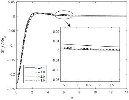
ticle concentration is substantially decreased with in- Figure 26 display the effect of Reaction rate, σ R , on
creasing Nb vales. The nanoparticles reorganize to create a the concentration distributions. A significant reduction in
new structure because of the spontaneous diffusivity. Thus concentration profiles is noted with rising σ values. An in-
the thermal conductivity of the nanofluid is improved. The crease in σ values results in an increase in the Arrhenius
Brownian motion warms the fluid in the boundary layer expression which eventually damages the chemical reac-
tion. Hence the concentration profiles decay.N. Vedavathi, Numerical study of radiative non-Darcy nanofluid flow | 171
Figure 28: Variations of Cf x for various M values
Figure 26: Variations of ϕ for various σ
Figure 29: Variations of Nu x for various M values
Figure 27: Variations of ϕ for various E
in the case of heat transfer rate. This confirms the earlier
Figure 27 illustrates the influence of Energy activa- observations that the flow is slowed by the magnetic field
tion number, E, on the concentration profiles. It is found but the fluid is heated. Higher heat transfer rates and a de-
that the concentration profiles increase with an increase crease in fluid temperature are associated with heat trans-
in E values. Usage of activation energy is more efficient fer from the fluid to the surface.
in enhancing the reaction process and hence increasing Figures 30 – 31 depicts the influences of radiation pa-
the concentration. The Arrhenius expression declines with rameter R on heat and mass transfer rates. A greater in-
an increase in E values, resulting in the development of crease in heat transfer rate is observed with a rise in ra-
the relational chemical reaction leading to an increase diation parameter whereas the mass transfer rate is de-
in the concentration profiles. Due to the phenomenon of creased. The flow is accelerated by the strong radiation,
low temperature and greater activation energy results in a but the heat transfer to the surface is reduced. Species dif-
lower reaction rate that slows down the chemical reaction. fusion to the surface is hampered by the greater contribu-
This way the concentration increases. tion of thermal conduction heat transfer.
Figures 28 – 29 depicts the influences of magnetic pa- Figure 32 – 33 depicts the influences of velocity slip
rameter M on skin friction and heat transfer rate. It has S and Darcy number K1 on skin friction. A significant de-
been seen that as the values of M increases, the skin fric- crease in skin friction is seen with an increase in velocity
tion increases near the wall and as we move away from the slip. With an increase in Darcy number the skin friction is
wall it decreases and a quite opposite trend is observed172 | N. Vedavathi, Numerical study of radiative non-Darcy nanofluid flow
Figure 30: Variations of Nu x for various R values Figure 33: Variations of Cf x for various K1 values
increased slightly near to the wall and as we move away
from the wall the skin friction is decreased.
Figure 31: Variations of Sh x for various R values
Figure 34: Variations of Nu x for various Fr values
Figure 34 presents the influences of Forchheimer num-
ber Fr on heat transfer rate. With an increase in Fr, the skin
friction is slightly decreased near the wall and as we move
away from the wall it is increased significantly.
Figure 35 illustrates the influences of Schmidt num-
ber Sc and reaction rate, σ R on mass transfer rate. The
mass transfer rate is increased with an increase in Sc val-
ues. While the mass transfer rate is decreased with an in-
crease in σ R values. An increase in Sc results in a decline in
species mass diffusivity and hence increases mass transfer
Figure 32: Variations of Cf x for various S values rate.N. Vedavathi, Numerical study of radiative non-Darcy nanofluid flow | 173
1. The fluid velocity is decreased with increasing values
of M whereas the fluid temperature and concentration
are increased.
2. Increasing mixed convection parameter elevates the
fluid velocity and nanoparticle concentration slightly
whereas temperature is slightly increased.
3. Increasing Darcy number is noted to reduce the fluid
velocity and nanoparticle concentration whereas tem-
perature is enhanced. A similar behavior is observed
with an increase in Forchheimer number and velocity
slip parameter.
4. Increasing Pr reduces the temperature and nanoparti-
cles concentration. Conversely, increasing Biot num-
ber enhances both temperature and nanoparticles
Figure 35: Variations of Sh x for various Sc values concentration.
5. Increasing radiation parameter enhances the fluid
temperature and nanoparticle concentration.
6. Increasing thermophoresis parameter strongly accel-
erates the nanoparticle concentration whereas in-
creasing Brownian motion parameter and Schmidt
number reduces nanoparticle concentration.
7. The nanoparticles concentration is decreased with in-
creasing reaction rate parameter whereas increased
slightly with increasing activation energy parameter.
Nomenclature:
a Positive constant associated with linear stretching
Bi Thermal Biot number
B0 Constant imposed magnetic field
Figure 36: Variations of Sh x for various σ values
C Concentration of the fluid
Cb Forchheimer inertial Drag coefficient
cp Specific heat parameter
5 Conclusion DT Thermophoretic diffusion constraint.
DB Brownian diffusivity
The present analytical study focuses on the thermally
Ea Activation energy
radiative electrically conducting Darcy-Forchheimer
E Energy activation number
Nanofluid flow characteristics past a stretching sheet
f Non-dimensional steam function
considering the effects of thermal conductivity, velocity
Fr Inertia-coefficient (Forchheimer number)
slip, convective heat transfer and Arrhenius activation
g Acceleration due to gravity
energy. The governing flow equations are converted into
hw Convective heat transfer coefficient
ordinary differential equations (ODE’s) with appropriate
k* Rosseland’s mean absorption coefficient
similarity transformations. Bvp4c technique is utilized in
k Thermal conductivity
order to obtain the results. The present numerical code is
K* Permeability
validated with the previous results available in literature.
K1 Darcy parameter
The influences of various flow controlled parameters on
Kc Reaction rate
velocity, temperature and nanoparticle volume fraction
L The parameter related to velocity slip
as well as shear stress rate, local Sherwood and Nusselt
n motile density
numbers presented and numerically and graphically. The
M Hartmann number
observations of as follows:
Nr Buoyancy parameter174 | N. Vedavathi, Numerical study of radiative non-Darcy nanofluid flow
Nb Brownian motion Constraint
Nt Thermophoresis parameter
References
Pr Prandtl number [1] Buongiorno J. Convective transport of nanofluids. J Heat Trans-
qr Radiative heat flux fer. 2006;128(3):240–50.
R Radiation parameter [2] Ellahi R, Zeeshan A, Shehzad N, Alamri SZ. Structural Impact
S Velocity slip parameter of Kerosene-Al2 O3 Nanoliquid on MHD Poiseuille Flow with
Sc Schmidt number Variable Thermal Conductivity: Application of Cooling Process.
J Mol Liq. 2018;264:607–15.
T Temperature of Nanofluid
[3] Choi SU. Enhancing thermal conductivity of fluids with
Tw convective fluid temperature nanoparticles, Developments and applications of non-
u, v The velocity components along (x, y) directions Newtonian flows. Siginer DA, Wang HP (Eds.). FED-The Amer-
ican Society of Mechanical Engineers. 1995;231/MD(66):99-
105.
[4] Patil PM, Shashikant A, Momoniat E. Transport phenomena in
Greek symbols
MHD mixed convective nanofluid flow. Int J Numer Methods
Heat Fluid Flow. 2020;30(2):769–91.
βT Thermal expansion coefficient [5] Khan NS, Shah Q, Bhaumik A, Kumam P, Thounthong P, Amiri
βc Concentration expansion coefficient I. Entropy generation in bioconvection nanofluid flow between
λ The buoyancy or mixed convective parameter two stretchable rotating disks. Sci Rep. 2020 Mar;10(1):4448.
ρf Base fluid density [6] Nainaru Tarakaramu PV. Satya Narayana and Bhumarapu
Venkateswarlu, Numerical simulation of variable thermal
(ρc)p Effective nano particles heat capacity
conductivity on 3D flow of nanofluid over a stretching sheet.
ρp Nanoparticle density Nonlinear Eng. 2020;9(1):233–43.
ν Kinematics viscosity [7] Shiriny A, Bayareh M, Ahmadi Nadooshan A. Nanofluid flow
σ Electric conductivity of the fluid in a microchannel with inclined cross-flow injection. SN Appl.
(ρc)f Fluid heat capacity Sci. 2019;1(9):1015.
[8] Suhail Ahmad Khan D, Altamush Siddiqui M. Numerical stud-
αf Thermal diffusivity
ies on heat and fluid flow of nanofluid in a partially heated
σR Reaction rate constant vertical annulus. Heat Transfer. 2020;49(3):1458–90.
δ Temperature difference parameter [9] Abdul Gaffar S, Ramachandra Prasad V, Rushi B, Anwar Beg O.
σ* Stefan-Boltzmann constant Computational solutions for mixed convection boundary layer
θ Non-dimensional temperature flows of Nanofluid from a non-isothermal wedge. J Nanofluids.
φ Non-dimensional concentration 2018;7(5):1024–32.
[10] Abdul Gaffar S, Ramachandra Prasad V, Ramesh Reddy P. Hi-
ψ Dimensionless stream function
dayathulla Khan, Venkatadri K, Magnetohydrodynamic Non-
η The dimensionless radial coordinate Darcy Flows of Nanofluid from Horizontal circular permeable
µ Dynamic viscosity cylinder: A Buongiorno’s mathematical model. J Nanofluids.
2019;8(2):276–86.
[11] Ghasemi SE, Hatami M. Solar radiation effects on MHD stagna-
tion point flow and heat transfer of a nanofluid over a stretch-
Subscripts
ing sheet. Case Stud Therm Eng. 2021;25:100898.
[12] Alfvén H. Existence of electromagnetic-hydrodynamic waves.
∞ Free stream condition Nature. 1942;150(3805):405–6.
w wall condition [13] Sing K, Pandey AK, Kumar M. Melting heat transfer assess-
ment on magnetic nanofluid flow past a porous stretching
Funding information: The authors state no funding cylinder. J Egypt Math Soc. 2021;29(1):1.
involved. [14] Basant K. Jha, Peter B. Malgwi, Hall and ion-slip effects
on MHD mixed convection flow in a vertical microchan-
nel with asymmetric wall heating. Engineering Reports.
Author contributions: All authors have accepted re- 2020;2(9):e12241.
sponsibility for the entire content of this manuscript and [15] Mohidul Haque M. Heat and Mass Transfer Analysis on Mag-
approved its submission. neto Micropolar Fluid Flow with Heat Absorption in Induced
Magnetic Field. Fluids. 2021;6(3):126.
[16] Alam J, Murtaza G, Tzirtzilakis E, Ferdows M. Jahangir Alam,
Conflict of interest: The authors state no conflict of inter-
Ghulam Murtaza, Efstratios Tzirtzilakis and Mohammad Fer-
est. dows, Biomagnetic Fluid Flow and Heat Transfer Study of
Blood with Gold Nanoparticles over a Stretching Sheet in the
Presence of Magnetic Dipole. Fluids. 2021;6(3):113.
[17] Md B. Hidayathulla Khan, S. Abdul Gaffar, Khalil-Ur-Rehman &N. Vedavathi, Numerical study of radiative non-Darcy nanofluid flow | 175
O. Anwar Beg, Entropy generation in magnetohydrodynamic 2020;2292:020001.
radiative non-Newtonian Dissipative convection flow From an [33] Jawad M. Anwar Saeed, Aurungzeb Khan, Saeed Islam, MHD
inclined plane: Numerical study, Nanoscience and Technology. bioconvection Darcy-Forchheimer flow of Casson nanofluid
Int J. 2020;11(4):297–326. over a rotating disk with entropy optimization. Heat Transfer;
[18] Vedavathi N, Dharmaiah G, Abdul Gaffar S, Venkatadri K. En- 2020. pp. 1–29.
tropy analysis of magnetohydrodynamic nanofluid transport [34] Zhang L, Bhatti MM, Michaelides EE. Electro-
from an inverted cone: Buongiorno’s model. Heat Transfer magnetohydrodynamic flow and heat transfer of a third-grade
Journal; 2020. https://doi.org/10.1002/htj.22021. fluid using a Darcy-Brinkman-Forchheimer model. Int J Numer
[19] Khan M, Rasheed A, Salahuddin T. Radiation and chemical Methods Heat Fluid Flow. 2020;ahead-of-print ahead-of-print:
reactive impact on tangent hyperbolic fluid flow having double https://doi.org/10.1108/HFF-09-2020-0566.
stratification. AIP Adv. 2020;10(7):075211. [35] Khan U, Zaib A, Baleanu D, Sheikholeslami M, Wakif A. Explo-
[20] Tunde A. Yusuf, Fazle Mabood, B. C. Prasannakumara and ration of dual solutions for an enhanced cross liquid flow past
Ioannis E. Sarris, Magneto-Bioconvection Flow of Williamson a moving wedge under the significant impacts of activation
Nanofluid over an Inclined Plate with Gyrotactic Microorgan- energy and chemical reaction. Heliyon. 2020 Jul;6(7):e04565.
isms and Entropy Generation. Fluids. 2021;6(3):109. [36] Aldabesh A, Ullah Khan S, Habib D, Waqas H, Tlili I, Ijaz Khan
[21] Jawad M, Saeed A, Tassaddiq A, Khan A, Gul T, Kumam P, et M, et al. Sami Ullah Khan, Danial Habib, Hassan Waqas,
al. Insight into the dynamics of second grade hybrid radiative Iskander Tlili, M. Ijaz Khan, Waqar Azeem Khan, Unsteady
nanofluid flow within the boundary layer subject to Lorentz transient slip flow of Williamson nanofluid containing gy-
force. Sci Rep. 2021 Mar;11(1):4894. rotactic microorganism and activation energy. Alex Eng J.
[22] Ge-JiLe H, Nazeer M, Hussain F, Khan MI, Saleem A, Siddique I. 2020;59(6):4315–28.
Hu Ge-JiLe, Mubbashar Nazeer, Farooq Hussain, M Ijaz Khan, [37] Ali M, Shahzad M, Sultan F, Khan WA, Rashid S. Exploring
Adila Saleem and Imran Siddique, Two-phase flow of MHD the features of stratification phenomena for 3D flow of Cross
Jeffrey fluid with the suspension of tiny metallic particles in- nanofluid considering activation energy. Int Commun Heat
corporated with viscous dissipation and Porous Medium. Adv Mass Transf. 2020;116:104674.
Mech Eng. 2021;13(3):1–15. [38] Khan SU, Waqas H, Muhammad T, Imran M, Aly S. Simulta-
[23] Jawad M, Saeed A, Khan A, Ali I, Alrabaiah H, Gul T, et al. neous effects of bioconvection and velocity slip in three-
Analytical study of MHD mixed convection flow for Maxwell dimensional flow of Eyring-Powell nanofluid with Arrhenius
nanofluid with variable thermal conductivity and Soret and activation energy and binary chemical reaction. Int Commun
Dufour effects. AIP Adv. 2021;11(3):035215. Heat Mass Transf. 2020;117:104738.
[24] Darcy H. Les Fontaines Publiques De La Ville De Dijon. Paris: [39] Khan MI, Alzahrani F, Hobiny A, Ali Z. Estimation of en-
Victor Dalmont; 1856. tropy generation in Carreau-Yasuda fluid flow using chem-
[25] Forchheimer P. Wasserbewegung durch boden. Z Ver D Ing. ical reaction with activation energy. J Mater Res Technol.
1901;45:1782–8. 2020;9(5):9951–64.
[26] Pop I, Ingham DB. Mathematical and Computational Modeling [40] Naganthran K, Zeeshan A, Md Basir MdF, Shehzad N, Nazar
of Viscous Fluids and Porous Media. Convective Heat Transfer. R, Choudhary R et al. Concentration Flux Dependent on Ra-
Oxford: Pergamon; 2001. diative MHD Casson Flow with Arrhenius Activation Energy:
[27] Vafai K. Handbook of Porous Media. 2nd ed. Homotopy Analysis Method (HAM) with an Evolutionary Al-
New York: Taylor and Francis Group; 2005. gorithm. Int J Heat Technol. 2020;38(4):785-793, 2020.
https://doi.org/10.1201/9780415876384. https://doi.org/10.18280/ijht.380403.
[28] Hayat T, Aziz A, Muhammad T, Alsaedi A. Effects of binary [41] Waqas H, Farooq U, Ibrahim A, Shah Z, Kumam P. Numerical
chemical reaction and Arrhenius activation energy in Darcy– Simulation of Bioconvectional flow of Burger Nanofluid with
Forchheimer three-dimensional flow of nanofluid subject to effects of Activation energy and Exponential Heat Source/Sink
rotating frame. J Therm Anal Calorim. 2019;136(4):1769–79. over an Inclined Wall under the Swimming Microorgan-
[29] Mir Asma WA. Othman, Taseer Muhammad, Numerical Study isms. Sci Rep. 2021. https://doi.org/10.21203/rs.3.rs-
for Darcy-Forchheimer flow of Nanofluid due to a Rotating 146009/v1.
Disk with Binary Chemical Reaction and Arrhenius Activation [42] Dawar A, Islam S, Shah Z, Kumam P. Significance of Mixed
Energy. Mathematics. 2019;7(10):921. Convection and Arrhenius Activation Energy in a Non-
[30] Muhammad Ramzan, Nomana Abid, Dianchen Lu and Iskan- Newtonian Third Grade Fluid Flow Containing Gyrotactic Mi-
der Tlili, Impact of melting heat transfer in the timedependent croorganisms towards Stretching Surface, Scientific Reports,
squeezing nanofluid flow containing carbon nanotubes in 2021. https://doi.org/10.21203/rs.3.rs-146062/v1.
a Darcy-Forchheimer porous media with Cattaneo-Christov [43] Wang CY. Free convection on a vertical stretching surface
heat flux, Commun. Theor. Phys. 2020;72:085801(11pp) [ZAMM] J Appl Math Mech. 1989;69:418–20.
https://doi.org/10.1088/1572-9494/ab8a2c.. [44] Gorla RS, Sidawi I. Free convection on a vertical stretching sur-
[31] Ahmad S, Ali K, Rizwan M, Ashraf M. Heat and Mass Trans- face with suction and blowing. Appl Sci Res. 1994;52(3):247–
fer Attributes of Copper-Aluminum Oxide Hybrid Nanoparti- 57.
cles Flow through a Porous Medium. Case Stud Therm Eng. [45] Khan WA, Pop I. Boundary-layer flow of a nanofluid past a
2021;25:100932. stretching sheet. Int J Heat Mass Transf. 2010;53(11-12):2477–
[32] Rabiha S. Kareem, and Ahmed M. Abdulhadi, A study 83.
of MHD and Darcy-Forchheimer effects on third grade [46] Shampine LF, Gladwell I, Thompson S. Solving ODEs with
flow with Cattaneo-Christov heat flux. AIP Conf Proc. MATLAB. New York: Cambridge University Press; 2003.176 | N. Vedavathi, Numerical study of radiative non-Darcy nanofluid flow
https://doi.org/10.1017/CBO9780511615542.
[47] Ibrahim W. Passive control of nanoparticle of micropolar fluid
past a stretching sheet with nanoparticles, convective bound-
ary condition and second-order slip. Proc IMechE Part E: J
Process Mechanical Engineering. 2017;231(4):704–19.You can also read