Observational constraints on Myrzakulov gravity - arXiv
←
→
Page content transcription
If your browser does not render page correctly, please read the page content below
Observational constraints on Myrzakulov gravity

                                         Fotios K. Anagnostopoulosa Spyros Basilakosb,c Emmanuel N. Saridakisc,d,e
                                         a
                                           Department of Physics, National & Kapodistrian University of Athens, Zografou Campus GR 157 73,
                                           Athens, Greece
                                         b
                                           Academy of Athens, Research Center for Astronomy and Applied Mathematics, Soranou Efesiou 4, 11527,
                                           Athens, Greece
                                         c
                                           National Observatory of Athens, Lofos Nymfon, 11852 Athens, Greece
                                         d
                                           CAS Key Laboratory for Researches in Galaxies and Cosmology, Department of Astronomy, University of
arXiv:2012.06524v2 [gr-qc] 11 May 2021

                                           Science and Technology of China, Hefei, Anhui 230026, P.R. China
                                         e
                                           School of Astronomy, School of Physical Sciences, University of Science and Technology of China, Hefei
                                           230026, P.R. China
                                             E-mail: fotis-anagnostopoulos@hotmail.com,
                                             svasil@academyofathens.gr, msaridak@noa.gr

                                         A BSTRACT: We use data from Supernovae (SNIa) Pantheon sample, from Baryonic Acoustic
                                         Oscillations (BAO), and from cosmic chronometers measurements of the Hubble parameter (CC),
                                         alongside arguments from Big Bang Nucleosynthesis (BBN), in order to extract constraints on
                                         Myrzakulov F(R, T ) gravity. This is a connection-based theory belonging to the Riemann-Cartan
                                         subclass, that uses a specific but non-special connection, which then leads to extra degrees of
                                         freedom. Our analysis shows that both considered models lead to ∼ 1σ compatibility in all cases.
                                         For the involved dimensionless parameter we find that it is constrained to an interval around zero,
                                         however the corresponding contours are slightly shifted towards positive values. Furthermore, we
                                         use the obtained parameter chains so to reconstruct the corresponding Hubble function, as well
                                         as the dark-energy equation-of-state parameter, as a function of redshift. As we show, Model 1
                                         is very close to ΛCDM scenario, while Model 2 resembles it at low redshifts, however at earlier
                                         times deviations are allowed. Finally, applying the AIC, BIC and the combined DIC criteria, we
                                         deduce that both models present a very efficient fitting behavior, and are statistically equivalent
                                         with ΛCDM cosmology, despite the fact that Model 2 does not contain the latter as a limit.

                                         K EYWORDS : Modified gravity, Observational Constraints, Torsional Gravity
Contents
1 Introduction 1
2 Myrzakulov Gravity and Cosmology 2
2.1 Myrzakulov Gravity 2
2.2 Cosmology 4
2.2.1 Model 1 5
2.2.2 Model 2 6
3 Data and Methodology 7
3.1 Cosmological probes 7
3.1.1 Direct measurements of the Hubble expansion 7
3.1.2 Supernovae Type Ia 7
3.1.3 Baryonic Acoustic Oscillations 8
3.1.4 Big Bang Nucleosynthesis 9
3.1.5 Joint likelihood analysis 9
3.2 Information Criteria and Model Selection 10
4 Results 11
5 Conclusions 16
1 Introduction
According to the concordance cosmological model the universe experienced two epochs of accel-
erated expansion, one at early and one at late times. Although the latter can be explained by the
presence of a cosmological constant, the related theoretical problem, the possibility of a dynamical
behavior, and especially the inability of the cosmological constant to describe the early accelerated
phase, led to the incorporation of some form of modification. As a first possibility one can main-
tain general relativity as the underlying theory and modify the matter content of the universe by
introducing extra fields, such as the inflaton at early times [1, 2] and/or the dark energy sector at
late times [3, 4]. As a second possibility one modifies the gravitational sector itself, constructing
a theory that possesses general relativity as a particular limit but which in general exhibits extra
degrees of freedom [5, 6].
There are many ways to construct gravitational modifications, each one modifying a particular
feature of general relativity. Modifying the dimensionality gives rise to the braneworld theories
[7], modifying the Einstein-Hilbert Lagrangian, gives rise to F(R) gravity [8, 9], F(G) gravity
[10, 11], Lovelock theories [12, 13], etc, while adding a scalar field coupled with curvature in
various ways gives rise to Horndeski/Galileon theories [14–16]. Additionally, starting from the
–1–equivalent, teleparallel, formulation of gravity [17, 18] one can construct modifications using tor-
sional invariants, such as in F(T ) gravity [19, 20], in F(T, TG ) gravity [21], or in scalar-torsion
theories [22, 23]. Moreover, one can construct the general class of metric-affine theories [24–26],
which incorporates a general linear connection structure, or proceed to the introduction of non-
linear connections such as in in Finsler and Finsler-like theories [27–32].
Inspired by these, one could start from such affinely connected metric theories, and in particu-
lar from their Riemann-Cartan subclass [33], and construct a theory using a specific but non-special
connection, which would lead to non-zero torsion and non-zero curvature at the same time, and
thus offering the extra degrees of freedom typically needed in any gravitational modification [34].
Myrzakulov gravity can thus lead to a good phenomenology, being able to describe the universe
evolution at early and late times [35–39].
One basic question in modified gravities is the determination of the arbitrary function that
enters in the theory. Although some general features can be deduced through theoretical consider-
ations, such as the absence of ghosts and instabilities, or the existence of Noether symmetries, the
most powerful tool is the use of observational data [40–60]. Hence, in this work we are interested
in using expansion data such as Supernovae type Ia data (SNIa), Baryonic Acoustic Oscillations
(BAO), and Hubble Cosmic Chronometers (CC) observations, in order to impose constraints on
Myrzakulov gravity. The plan of the work is the following. In Section 2 we present Myrzakulov
gravity and its cosmological applications. In Section 3 we describe the various datasets and the
involved statistical methods. Then in Section 4 we preform our analysis and we present the re-
sults, namely the constraints on the various parameters. Finally, in Section 5 we summarize and
conclude.
2 Myrzakulov Gravity and Cosmology
In this section we present a brief review of Myrzakulov gravity, or F(R, T ) gravity [34, 35], ex-
tracting additionally the relevant cosmological equations.
2.1 Myrzakulov Gravity
The central idea of this modified gravity is the modification of the underlying connection. In
particular, it is known that imposing a general connection ωabc one defines the curvature and the
torsion tensor respectively as [21]
Rabµν = ωabν,µ − ωabµ,ν + ωacµ ωc bν − ωacν ωc bµ , (2.1)
T aµν = eaν,µ − eaµ,ν + ωabµ ebν − ωabν ebµ , (2.2)
µ
where ea ∂µ is the tetrad field related to the metric through gµν = ηab eaµ ebν , where ηab =
diag(1, −1, −1, −1), with Greek and Latin indices denoting coordinate and tangent space respec-
tively, and where comma denotes differentiation.
There are infinite connection choices. The Levi-Civita Γabc is the only connection that gives
vanishing torsion, and from now on we use the label “LC” to denote the curvature (Riemann) tensor
corresponding to Γabc , namely R(LC)abµν = Γabν,µ − Γabµ,ν + Γacµ Γc bν − Γacν Γc bµ . On the other hand
one can use the Weitzenböck connection W λµν = eaλ eaµ,ν which is curvatureless, leading only to
–2–torsion as T (W)λµν = W λνµ − W λµν (we use the label “W” to denote quantities corresponding to W λµν .
From the above it is implied that the Ricci scalar corresponding to the Levi-Civita connection is
µ ρ ρ
R(LC) = ηab ea ebν Γλµν,λ − Γλµλ,ν + Γ µν Γλλρ − Γ µλ Γλνρ ,
h i
(2.3)
while the torsion scalar corresponding to the Weitzenböck connection is
1 µλν 1
W − W µνλ Wµλν − Wµνλ + W µλν − W µνλ Wλµν − Wλνµ
T (W) =
4 2
µν νµ λ λ
− Wν − Wν W µλ − W λµ . (2.4)
As it is known, the former is used in the Lagrangian of General Relativity and in all curvature-based
modified gravities, e.g. in F(R) gravity [8], while the latter is used in the Lagrangian of teleparallel
equivalent of general relativity and in all torsion-modified gravities, e.g. in F(T ) gravity [6].
In Myrzakulov gravity one uses a non-special connection which has non-zero curvature and
torsion simultaneously [35]. Hence, the resulting theory will in general possess extra degrees of
freedom, even if the imposed Lagrangian is simple, which is not the case of general relativity or of
teleparallel equivalent of general relativity that both have two degrees of freedom corresponding to
the massless graviton. The action of the theory is
Z " #
F(R, T )
S = 4
d xe + Lm , (2.5)
2κ2
√
where e = det(eaµ ) = −g, κ2 = 8πG is the gravitational constant, and where we have introduced
the matter Lagrangian Lm too for completeness. Note that in the arbitrary function F(R, T ) the
R and T are the curvature and torsion scalars corresponding to the non-special connection used,
which read as [21]
1 1 νµ
T = T µνλ T µνλ + T µνλ T λνµ − T ν T λλµ , (2.6)
4 2
νµ
R = R(LC) + T − 2T ν ;µ , (2.7)
where ; marks the covariant differentiation with respect to the Levi-Civita connection. Therefore,
T depends on the tetrad field, its first derivative and the connection, while R depends on the tetrad
and its first derivative, and on the connection and its first derivative, with an additional dependence
on the second tetrad derivative due to the last term of (2.7). Thus, using (2.4),(2.6),(2.7) we can
finally write
T = T (W) + v, (2.8)
R=R (LC)
+ u, (2.9)
where v is a scalar depending on the tetrad, its first derivative and the connection, while u is a scalar
depending on the tetrad, its first and second derivatives, and the connection and its first derivative.
The quantities u and v quantify the effect of the specific but non-special imposed connection.
In the case where this connection becomes the Levi-Civita one, then u = 0 and v = −T (W) , and the
above theory becomes the usual F(R) gravity, which in turn coincides with general relativity under
F(R) = R. On the other hand, in the case where the connection is the Weitzenböck one, then we
have that v = 0 and u = −R(LC) and hence the theory coincides with F(T ) gravity, which in turn
becomes the teleparallel equivalent of general relativity for F(T ) = T .
–3–2.2 Cosmology
Let us now apply the above into a cosmological framework and extract the corresponding equations
that determine the universe evolution. As it was shown in [35], in order to avoid complications
related to the additional variation in terms of the connection, it proves convenient to apply a mini-
super-space procedure. Hence, we apply the homogeneous and isotropic flat Friedmann-Robertson-
Walker (FRW) geometry
ds2 = dt2 − a2 (t) δi j dxi dx j , (2.10)
which corresponds to the tetrad eaµ = diag[1, a(t), a(t), a(t)], where a(t) is the scale factor. In this
2 2
case one can easily find that R(LC) = 6 äa + ȧa2 and T (W) = −6 aȧ2 . Furthermore, we use the
standard replacement Lm = −ρm (a) [61–63]. Lastly, following the discussion on the dependence of
u and v above, we consistently impose that u = u(a, ȧ, ä) and v = v(a, ȧ).
In this work we are interested in exploring the cosmological behavior that arise purely from
the non-special connection of Myrzakulov gravity. Hence, we focus on the simplest case where the
involved arbitrary function is trivial, namely F(R, T ) = R + λT with λ a dimensionless parameter
(we omit the coupling coefficient of R since it can be absorbed into κ2 ). Note that we do not
consider an explicit cosmological constant term in the Lagrangian. Inserting the above R mini-super-
space expressions into the action (2.5), for this Lagrangian choice we acquire S = Ldt, where
3 a3
L= [λ + 1] aȧ 2
− [u(a, ȧ, ä) + λv(a, ȧ)] + a3 ρm (a). (2.11)
κ2 2κ2
∂L ∂ ∂L
h i
Extracting the equations of motion for a, alongside the Hamiltonian constraint H = ȧ ∂ȧ − ∂t ∂ä +
ä ∂L
∂ä − L = 0, we finally acquire the Friedmann equations
3H 2 = κ2 (ρm + ρde ) (2.12)
2Ḣ + 3H 2 = −κ2 (pm + pde ) , (2.13)
where
" #
1 Ha 1 auä
ρde = 2 (uȧ + vȧ λ) − (u + λv) + 2
Ḣ − 2H − 3λH 2
(2.14)
κ 2 2 2
"
1 Ha 1 a
pde = − 2 (uȧ + vȧ λ) − (u + λv) − (ua + λva − u̇ȧ − λv̇ȧ )
κ 2 2 6
a a
− Ḣ + 3H 2 uä − Hau̇ä − üä − λ(2Ḣ + 3H 2 ) , (2.15)
2 6
with H = ȧa the Hubble parameter, pm the matter pressure, and with the subscripts a, ȧ, ä denoting
partial derivatives with respect to this argument. Hence, in the theory at hand, we obtain an effective
dark energy sector which arises from the non-special connection. Additionally, given the matter
conservation equation ρ̇m + 3H(ρm + pm ) = 0 we find
ρ̇de + 3H(ρde + pde ) = 0, (2.16)
which implies that the effective dark energy sector is conserved.
–4–The above Friedmann equations can efficiently describe the late-time acceleration. A first
observation is that in the case where λ = 0, namely in the case where the Lagrangian is just the cur-
vature (nevertheless the non-special connection leads to non-zero torsion too), and for the choice
u = c1 ȧ − c2 , with c1 ,c2 constants, then we have ρde = −pde = 2κc22 ≡ Λ. Hence, the scenario at hand
includes ΛCDM cosmology as a sub-case, although we have not considered an explicit cosmologi-
cal constant, since the cosmological constant arises effectively from the connection structure of the
theory. Thus, we expect that a realistic model would be a deviation from the above scenario.
Finally, it proves convenient to introduce the decceleration parameter as
Ḣ
q = −1 − , (2.17)
H2
which quantifies the cosmic acceleration. Defining additionally the density parameters Ωm =
κ2 ρm /(3H 2 ) and Ωde = κ2 ρde /(3H 2 ), as well as the equation-of-state parameters wm ≡ pm /ρm
and wde ≡ pde /ρde , we can extract the useful expression
2q − 1
= Ωm wm + Ωde wde . (2.18)
3
Hence, in the standard case of dust matter, namely for wm ≈ 0, we obtain
2q − 1
wde = . (2.19)
3(1 − Ωm )
This expression allows one to find the evolution of the dark energy equation-of-state parameter,
knowing the solution of the Friedmann equations, or knowing the observable values of H(z) (where
z is the redshift defined through 1 + z = a0 /a setting the current value of the scale factor to a0 = 1).
In the following we will focus to two models which can satisfy these features.
2.2.1 Model 1
Choosing u = c1 ȧ − c2 and v = c3 ȧ − c4 , with c3 ,c4 constants, we obtain
3H 2 = κ2 (ρm + ρde ) (2.20)
2Ḣ + 3H = −κ (pm + pde ) ,
2 2
(2.21)
with
1 h i
ρde = c − 3λH 2
(2.22)
κ2
1 h i
pde = − 2 c − λ(2Ḣ + 3H 2 ) , (2.23)
κ
where c ≡ c2 + c4 . Hence, in this scenario the geometrical sector constitutes an effective dark
energy sector with the above energy density and pressure, and an equation-of-state parameter of
the form
2λḢ
wde = −1 + . (2.24)
c − 3λH 2
Interestingly enough, we can see that wde can be both larger or smaller than -1, and thus the effective
dark energy can be quintessence or phantom like.
–5–This model has two parameters, namely c, λ, but one of them can be eliminated using the
present value of the matter density parameter Ωm0 (from now on the subscript “0” denotes the
current value of a quantity), since (2.20) at present gives:
c
1 = Ωm0 + − λ. (2.25)
3H02
Additionally, the deceleration parameter (2.18), using (2.22),(2.23), becomes
2Ωm0 (1 + z)3
q(z) = −1 + , (2.26)
Ωm0 (1 + z)3 + 2(1 + λ − Ωm0 )
and thus its value at present is
3Ωm0
q0 = −1 + . (2.27)
2(1 + λ)
Comparing with the corresponding value of ΛCDM scenario, namely qΛ 0 = −1 + 3Ωm0 /2, we verify
that for the special case of λ = 0 the two scenarios coincide, as mentioned above. Finally, note that
from relation (2.26) we can calculate the transition redshit, namely the redshift in which q transits
from posotive to negative and we have the onset of acceleration, finding
ztr = −1 + 21/3 (1 + λ − Ωm0 )1/3 Ω−1/3
m0 . (2.28)
2.2.2 Model 2
As a second example let us consider a more general model with u = c1 aȧ ln ȧ and v = s(a)ȧ, with
s(a) an arbitrary function. In this case (2.14),(2.15) give
3H 2 = κ2 (ρm + ρde ) (2.29)
2Ḣ + 3H 2 = −κ2 (pm + pde ) , (2.30)
with
1 c1
ρde = H − 3λH 2
(2.31)
κ2 2" #
1 c1 c1 Ḣ
pde =− 2 H+ − λ(2Ḣ + 3H 2 ) , (2.32)
κ 2 6 H
while
c1 Ḣ
2λḢ − 6 H
wde = −1 + c1 . (2.33)
2H − 3λH 2
Similarly to the previous example, for this case too wde can be quintessence-like or phantom-like.
This model has two parameters, namely c1 , λ, but one of them can be eliminated using Ωm0 ,
since (2.20) at present time leads to:
c1
1 = Ωm0 + − λ. (2.34)
6H0
The deceleration parameter (2.18) becomes
2 Ωm0 (1 + z)3
3
q(z) = −1 + (2.35)
3(1 − Ωm0 + λ) + (1 + λ)−1 (1 − Ωm0 + λ)2 + (1 + λ)(1 + z)3 Ωm0 1/2
–6–and its current value is
2 Ωm0
3
q0 = −1 + . (2.36)
3(1 − Ωm0 + λ) + (1 + λ)−1 (1 − Ωm0 + λ)2 + (1 + λ)Ωm0 1/2
Finally, from relation (2.35) we can calculate the transition redshit as
61/3 (1 + λ)−1/3 Ω−1/3
m0
ztr = −1 +
n 3
· 10 + 9λ(2 + λ − Ωm0 ) − 9Ωm0
q o1/3
− 28 − 36Ωm0 + 9[3λ(2 + λ) − 4λΩm0 + Ω2m0 ] . (2.37)
3 Data and Methodology
In this section we describe the various datasets that are going to be used in our analysis, and also
the involved statistical methods. In particular, we will use data from direct measurements of the
Hubble parameter, from Supernovae Type Ia (SNIa), and from Baryonic Acoustic Oscillations.
Finally, we present various information criteria that offer information on the quality of the fit.
3.1 Cosmological probes
3.1.1 Direct measurements of the Hubble expansion
From the latest H(z) data set compilation available in Ref. [64] we use only data obtained from
cosmic chronometers (CC). By using the differential age of passive evolving galaxies one can mea-
sure the Hubble rate directly (see e.g. Ref. [66] and references therein). These galaxies are massive
galaxies that evolve “slowly” at certain intervals of the cosmic time, i.e with small fraction of “new”
stars. A striking advantage of the differential age of passive evolving galaxies is that the resulting
measurement of the Hubble rate comes without any assumptions for the underlying cosmology,
with the exception of imposed spatial flatness. Our study incorporates N = 31 measurements of
the Hubble expansion in the redshift range 0.07 . z . 2.0.
Here, the corresponding χ2H function reads
i2
N H obs − H (z ; φν )
h
th i
φν =
X i
χ2H ,
(3.1)
i=1
σ2i
where Hiobs is the observed Hubble rate at redshift zi and σi the corresponding uncertainty, while
φν is the statistical vector that contains the free parameters of the examined model.
3.1.2 Supernovae Type Ia
The most common class of cosmological probes is the so-called “standard” candles. The latter
are luminous extra-galactic astrophysical objects with observable features that are independent of
the cosmic time. The most known standard candles and probably the most thoroughly studied
are Supernovae Type Ia (SNIa). In our analysis we use the most recent SNIa dataset available,
i.e the binned Pantheon sample of Scolnic et. al. [67]. The full dataset is approximated very
–7–efficiently with the binned N = 40 data points belonging to the redshift interval 0.01 . z . 1.6.
The corresponding χ2 is
χ2S NIa φν+1 = µSNIa C−1
SNIa,cov µSNIa ,
T
(3.2)
where µSNIa = {µ1 − µth (z1 , φν ) , ... , µN − µth (zN , φν )}. The distance modulus reads as µi = µB,i − M,
with µB,i the apparent maximum magnitude for redshift zi . Here, M is a hyper-parameter [67] that
quantifies uncertainties of various origins, such as astrophysical ones, data-reduction pipeline, etc,
and it is employed instead of the usage of α, β free parameters, in the context of “BEAMS with
Bias Corrections” method [65]. The observed distance modulus is compared with the theoretical
one, i.e
dL (z; φν )
!
µth = 5 log + 25 , (3.3)
Mpc
with Z z
ν dx
dL (z; φ ) = c(1 + z) (3.4)
0 H(x, φν )
the luminosity distance for flat FRW geometry. It must be noted that M and the normalized Hubble
constant h are degenerate in light of Pantheon dataset in an intrinsic way, as it is usual in standard
candles. Therefore, one should jointly employ other data-sets in order to obtain meaningful infor-
mation regarding the present value H0 .
3.1.3 Baryonic Acoustic Oscillations
Baryonic Acoustic Oscillations refer to the imprint left by relativistic sound waves in the early
universe, providing an observable to the late-time large scale structure. The main idea is to measure
the aforementioned scale at different times (i.e redshifts), and thus obtain DA (z) and H(z). The
acoustic length scale corresponds to the co-moving distance that the sound waves could travel until
the recombination z∗ [68], namely Z ∞
c s (z)
rd = . (3.5)
z∗ H(z)
For the concordance model, the sound speed, c s , is given from an analytical expression. How-
ever, for the models considered here there is not such an expression, therefore the scale rd will
be addressed as a free parameter. Furthermore, distances of different objects along the line of
sight correspond to different redshifts and thus depend on the combination H(z)rd , while distances
transverse to the line of sight are related with the combination DA (z)/rd .
Employing large samples of tracers, (i.e galaxies), one can detect by statistical means the BAO
peak, (for details see [69] and references therein). In order to achieve this it is required to impose an
underlying cosmology, and hence the method is not model independent. However, the differences
that may infiltrate at the final data products are much less than the statistical errors, and in most
cases the data points are calibrated with the quantity rd, f id /rd . In this work we employ the BAOs
data-set used by [70], that consists of N = 11 data points in the redshift range 0.106 . z . 2.36.
The relevant χ2 function reads as
i2
N T (z ; φν ) − T obs
h
i
χ2BAO φν+1 = sCcov
X i
−1 T
s + , (3.6)
i=8
σ2i
–8–with Ccov−1 the inverse of the covariance matrix of the first 6 measurements available at [70]. The
vector s has as elements the si , given as si = dm − diobs rd /rd, f id for odd i and si = H(zi ; φν ) −
Hiobs rd, f id /rd for even i. In all cases, rd, f id = 147.78. Furthermore, for i ∈ {8, 9}, T (zi ; φν ) =
Dv (zi ; φν ), T iobs = Dobs
v,i rd /rd, f id , with r f id,8 = 148.69 M pc and r f id,9 = 147.66 M pc respectively.
For i = 10, T (zi ; φ ) = cH(zi ; φν )−0.7 Dm (zi ; φν )0.3 /rd and for i = 11, T (zi ; φν ) = cH(zi ; φν )−1 rd .
ν
Finally, in the expressions above the following quantities have been used
DL (zi ; φν )
D M (zi ; φν ) = , (3.7a)
1+z
DL (zi ; φν )
DA (zi ; φν ) = , (3.7b)
(1 + z)2
#1/3
cDA (z; φν )2 z(1 + z)2
"
ν
DV (z; φ ) = . (3.7c)
H(z; φν )
3.1.4 Big Bang Nucleosynthesis
Any cosmological scenario arising from modified gravity should preserve the standard thermal
history of the universe. Hence, a basic and rough condition is applicable in the form of an extra
prior. Specifically, we require that the following inequality holds [71–73]
(Hi (zBBN ; φν ) − HΛ (zBBN ; Ωm0 ))2
< 0.1, (3.8)
HΛ (zBBN ; Ωm0 )2
where zBBN ∼ 109 . For the fiducial ΛCDM cosmology, namely HΛ , we employ the parameter
values from Planck [74].
3.1.5 Joint likelihood analysis
In order to obtain the joint constraints on the cosmological parameters from the aforementioned
cosmological probes, we introduce the total likelihood function as
Ltot (φk ) = LS NIa × LH × LBAO . (3.9)
It is easy to deduce that relevant χ2tot is given as
χ2tot (φk ) = χ2S NIa + χ2H + χ2BAO . (3.10)
The involved statistical vector has k components, i.e. the ν parameters of the scenario at hand plus
νhyp hyper-parameters from the imposed datasets, namely k = ν+νhyp . Hence, the vector containing
the free parameters of the scenaria at hand is φk = {Ωm0 , h, λ, M, rd }. Note however that from a
statistical point of view there is no distinction between the intrinsic hyper-parameters of a given
dataset and the free parameters of a cosmological scenario.
Finally, for the likelihood maximization we use an affine-invariant Markov Chain Monte Carlo
sampler [75], obtained in the Python package emcee [76]. We use 1000 chains (walkers) and 3500
steps (states). As a prior we employ firstly the conditions 0.0 < Ωm0 < 1, 0.60 < h < 0.90,
−19.9 < M < −18.0, −0.9 < λ < 2.8, 135 < rd < 160, and secondly the BBN constraint
described above. Lastly, the convergence of the MCMC algorithm is verified with auto-correlation
time implementation, and moreover for completeness the Gelman-Rubin criterion is calculated.
–9–3.2 Information Criteria and Model Selection
As a last step we present the standard ways in order to compare a set of cosmological scenarios,
namely we apply the Akaike Information Criterion (AIC) [77], the Bayesian Information Crite-
rion (BIC) [78], and the Deviance Information Criterion [79]. Moreover, we present the standard
χ2min /dof, where “dof” stands for degrees of freedom, usually defined as the number of the used
data points minus the number of fitted parameters. In our case this gives dof=77. Nevertheless,
χ2min /dof should be used for illustrative purposes, as the degrees of freedom might be ambiguous
for non-linear (in terms of the free parameters) models. [80].
The AIC criterion is based on information theory and it is an asymptotically unbiased estima-
tor of the Kullback-Leibler information. Under the standard assumption of Gaussian errors, the
corresponding estimator for the AIC criterion reads [81, 82]
2k(k + 1)
AIC = −2 ln(Lmax ) + 2k + , (3.11)
Ntot − k − 1
with Lmax the maximum likelihood of the dataset(s) under consideration and Ntot the total data
points number. It is apparent that for Ntot >> 1 this expression gives the original AIC version,
namely AIC ' −2 ln(Lmax ) + 2k. As it is discussed in [83], it is considered as best practise to use
the modified AIC criterion.
The BIC criterion is a Bayesian evidence estimator, and it is written as [81–83]
BIC = −2 ln(Lmax ) + k log(Ntot ) . (3.12)
Finally, the DIC criterion employs both Bayesian statistics and information theory concepts [79],
and it is expressed as [83]
DIC = D(φk ) + 2C B . (3.13)
The quantity C B is the Bayesian complexity C B = D(φk ) − D(φk ), where overlines imply the
standard mean value. Moreover, D(φk ) is the Bayesian Deviation, which can be expressed as
D(φk ) = −2 ln[L(φk )] in the case of exponential class of distributions. It is closely related to the
number of effective degrees of freedom [79], which is actually the number of parameters that affect
the fitting. In a less strict manner, it could be considered as a measure of the “spread” of the
likelihood.
In contrast with AIC and BIC criteria, instead of using just the best fit likelihood, DIC uses the
whole sample. Furthermore, AIC and BIC count and penalize all the involved parameters, while
DIC penalizes only the number of parameters that contribute to the fit in an actual way. Finally, an
additional appealing feature of DIC criterion is that its calculation is computationally light under
the MCMC samples.
Given a set of scenarios that describe the same class of phenomena, our problem is to sort
the models according to their fitting efficiency in the context of the available data. We employ the
aforementioned three information criteria (IC) and we calculate the relative difference of the IC
value for the given set of models, ∆ICmodel = ICmodel − ICmin , where the ICmin is the minimum
IC value inside the competing models set. In order to qualify each model in terms of its relevant
adequacy, we apply the Jeffreys scale [84]. Specifically, the condition ∆IC ≤ 2 implies statistical
– 10 –Model Ωm0 h λ rd M χ2min χ2min /do f
Mod. 1 0.425+0.107
−0.146
0.691+0.016 +0.387 +2.55 +0.051
−0.017 0.491−0.533 146.20−3.41 −19.382−0.052 61.93 0.8043
Mod. 2 0.339+0.093 +0.016 +0.403 +3.57 +0.051
−0.122 0.679−0.016 0.537−0.550 146.60−3.44 −19.396−0.052 63.53 0.8251
ΛCDM 0.292+0.015 +0.017
−0.014 0.692−0.017 - 145.87+3.53 +0.051
−3.38 −19.377−0.052 61.73 0.7914
Table 1. Observational constraints and the corresponding χ2min , as well as χ2min /do f (where “dof” stands for
degrees of freedom, in our case dof = 77), for the two Myrzakulov gravity models, presented previously,
using CC/Pantheon/BAO data-sets. In order to allow direct comparison, the concordance flat ΛCDM model
is also analyzed, giving results very similar with the corresponding ones of [85].
compatibility with the most favoured model by the data, while the condition 2 < ∆IC < 6 corre-
sponds to middle tension between the two models, and lastly the condition ∆IC ≥ 10 implies strong
tension.
4 Results
In this section we proceed to the observational analysis of Myrzakulov gravity using the datasets
and the methods described above. Note that the free parameters of the aforementioned models are
Ωm0 , h and λ, while for the case of the concordance cosmology they are Ωm0 , h. For convenience
we summarize the obtained results in Table 1. Additionally, in Figs. 1 and 2 we present the
corresponding contour plots for Model 1 and Model 2 respectively. For comparison and benchmark
we also analyzed the concordance model, namely ΛCDM.
As we can see, according to the combined analysis of CC+SNIa+BAO data we acquire ∼ 1σ
compatibility in all cases. The dimensionless parameter λ is constrained to an interval around
0, that includes ΛCDM paradigm, which was expected since as we discussed above a realistic
modified gravity should be a small deviation from general relativity. Nevertheless, note that in both
Model 1 and Model 2, the λ-contours are slightly shifted towards positive values. We mention
that having the likelihood contours for the parameter λ allows us to extract the constraints on the
parameter c through expression (2.25) for Model 1 and on the parameter c1 through (2.34) for
Model 2. In particular, for 1σ region for Model 1 we obtain c = 1.550+0.828
−0.876
, while for Model 2 we
+2.28
find c1 = 4.94−2.75 .
Concerning the values of Ωm0 we observe that Model 1 gives a rather large value, due to the
degeneracy with λ, while for Model 2 this is not the case. Concerning the Hubble constant h,
for Model 1 we find that 0.690+0.016 +0.016
−0.017 , while for Model 2 we obtain 0.679−0.016 . This implies that
the obtained values for the present Hubble parameter H0 are in between the Planck estimation
H0 = 67.36 ± 0.54 km/s/Mpc [74] and the local estimation H0 = 73.24 ± 1.74 km/s/Mpc [86],
although closer to the former. In addition, the extracted H0 value for both models is consistent
with other astrophysical inferences of Hubble constant, i.e H0 = 67.4+4.1 −1
−3.2 kms M pc
−1 [87], and
H0 = 69.6 ± 2.5 kms−1 M pc−1 [88]. It is interesting to note that results in this range have been
supported for about a decade now, amongst others in [89–95].
In order to provide a more complete and transparent picture, we use the obtained allowed
parameter values in order to extract the resulting H(z). In Figs. 3 and 4 we present the reconstructed
mean H(z)/(z + 1) as a function of the redshift, alongside the allowed curves for the 1σ allowed
– 11 –m0 = 0.4350+0.1177
0.1560
h = 0.6908+0.0171
0.0169
6
0.7
2
0.7
h
8
0.6
4
= 0.4911+0.3872
0.6
0.5337
1.0
0.5
0.0
= 19.3829+0.0513
0.0521
.2 .5
19 0
.3
19
.4
19
.5
19
rd = 146.1955+3.5538
3.4067
.6
19
5
15
0
15
rd
5
14
0
14
5
0
5
0
5
4
8
2
6
0.5
0.0
0.5
1.0
.6
.5
.4
.3
.2
0
5
0
5
0.1
0.3
0.4
0.6
0.7
0.6
0.6
0.7
0.7
14
14
15
15
19
19
19
19
19
m0 h rd
Figure 1. The 1σ, 2σ and 3σ likelihood contours for Model 1 of (2.22),(2.23), for all possible 2D subsets of
the parameter space (Ωm0 , h, λ, M, rd ). Moreover, we present the mean parameter values within the 1σ area
of the MCMC chain. We have performed a joint analysis of CC+SNIa+BAO data.
model parameters presented above, for Model 1 and Model 2 respectively. These graphs are quite
similar with the corresponding ones for quintessence models (φCDM) of [96].
As a next step we investigate of the evolution of the dark energy equation-of-state parameter.
In particular, having obtained the allowed parameter values at 1σ confidence level, we can use them
in order to extract the resulting wde (z) behavior given by (2.19), with the deceleration parameter
– 12 –m0 = 0.3411+0.0939
0.1222
h = 0.6793+0.0169
0.0168
3 6 9 2 5
0.6 0.6 0.6 0.7 0.7
h
= 0.5371+0.4035
0.5502
1.5
1.0
0.5
0.0
= 19.3962+0.0514
0.0524
.2 .5
19 0
.3
19
.4
19
.5
19
rd = 146.5991+3.5766
3.4461
.6
19
5
15
0
15
rd
5
14
0
14
5
0
5
0
3
6
9
2
5
0.5
0.0
0.5
1.0
1.5
.6
.5
.4
.3
.2
0
5
0
5
0.1
0.3
0.4
0.6
0.6
0.6
0.6
0.7
0.7
14
14
15
15
19
19
19
19
19
m0 h rd
Figure 2. The 1σ, 2σ and 3σ likelihood contours for Model 2 of (2.31),(2.32), for all possible 2D subsets of
the parameter space (Ωm0 , h, λ, M, rd ). Moreover, we present the mean parameter values within the 1σ area
of the MCMC chain. We have performed a joint analysis of CC+SNIa+BAO data.
given by (2.26) for Model 1 and by (2.35) for Model 2.
In Fig. 5 we depict the reconstructed mean wde (z) (red curve) for Model 1, alongside the
allowed curves for the 1σ allowed model parameters presented above. As we observe, the corre-
sponding behavior is very close to ΛCDM scenario for every parameter values. Similarly, in Fig.
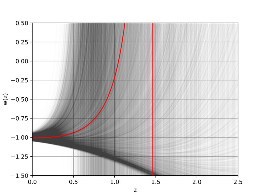
6 we present the corresponding graph for Model 2. In this case the scenario resembles ΛCDM
at low redshifts, however at earlier times the mean curve, as well as many of the “individual”
– 13 –Figure 3. The reconstruction of the H(z)/(z + 1) as a function of the redshift for Model 1, arisen from
(2.20),(2.22). We re-sampled the chains produced by emcee taking 6000 samples, and we plot all the ob-
tained curves, alongside the curve corresponding to the best fit of the parameters (red curve).
Figure 4. The reconstruction of the H(z)/(z + 1) as a function of the redshift for Model 2, arisen from
(2.29),(2.31). We re-sampled the chains produced by emcee taking 6000 samples, and we plot all the ob-
tained curves, alongside the curve corresponding to the best fit of the parameters (red curve).
– 14 –Figure 5. The reconstruction of the effective dark-energy equation-of-state parameter wde (z) as a function of
the redshift for Model 1 given by (2.24). We re-sampled the chains produced by emcee taking 6000 samples,
and we plot all the obtained wde (z) curves, alongside the curve corresponding to the best fit of the parameters
(red curve).
curves, present a deviation, since this is allowed by the used datasets. In particular, for some pa-
rameter choices the dark-energy pressure at a particular redshift diverges and changes sign, and
thus the wde (z) transits on the other side of the phantom-divide. Such energy conditions violations
are common in modified gravity theories, and actually they can lead to interesting cosmological
phenomenology. Note that the observable quantities (the Hubble function and its derivatives, the
density parameters etc) remain finite. However, we mention that a significant sub-set of the curves,
i.e. a large region of the parameter space of the model, does not exhibit such a behavior, and the
individual obtained curves resemble the ΛCDM evolution.
Furthermore, we proceed to the reconstruction of the decceleration parameter using random
sampling of the obtained chains. Concerning the current value q0 , for Model 1 using (2.27) we
obtain q0 = −0.561+0.022 +0.010
−0.021 , while for Model 2 using (2.36) we acquire q0 = −0.880−0.009 . These
are in agreement with the values obtained using other datasets, such as supernovae, quasars and
gamma-ray bursts by means of model-independent techniques [97].
Additionally, we calculate the transition redshift, for the two models, using relations (2.28)
and (2.37) respectively. For Model 1 we find ztr,1 = 0.36+0.10 −0.18 , while for Model 2 we acquire
+0.07
ztr,2 = 0.74−0.14 . It is of interest to compare the aforementioned values with ztr,A = 0.72 ± 0.05,
[96] and ztr,B = 0.64+0.12
−0.09 , [98]. For Model 1 we observe mild compatibility within ∼ 3.5σ and
within ∼ 3σ with “A” and “B” results, respectively. On the other hand, for the case of Model 2 we
– 15 –Figure 6. The reconstruction of the effective dark-energy equation-of-state parameter wde (z) as a function
of the redshift for Model 2 given by (2.33). We re-sampled the chains produced by emcee taking 6000
samples, and we plot all the obtained wde (z) curves, alongside the curve corresponding to the best fit of
the parameters (red curve). The over-populated area at the bottom corresponds to a peak within 1σ area,
nevertheless since we extract the median value of each parameter within 1σ as the best fit, the “best” wde (z)
curve differs.
report 1 σ compatibility with both results. These results act as an additional verification check of
the examined models.
We close this analysis with the examination of the statistical significance of our fitting results,
applying the AIC, BIC and DIC information criteria described in subsection 3.2. We summarize
our results in Table 2. As we observe, Model 1 is statistically equivalent with ΛCDM paradigm, and
especially the combined and more complete DIC criterion gives an almost equal value. Addition-
ally, Model 2 also presents a very good fitting behavior, and according to DIC it is also statistically
equivalent with ΛCDM paradigm, which is an interesting result since Model 2 does not contain
ΛCDM scenario as a limit for any parameter value.
5 Conclusions
In this work we have used observational data from Supernovae (SNIa) Pantheon sample, from
Baryonic Acoustic Oscillations (BAO), and from cosmic chronometers measurements of the Hub-
ble parameter (CC), alongside arguments from Big Bang Nucleosynthesis (BBN), in order to ex-
tract constraints on Myrzakulov F(R, T ) gravity. This is a connection-based theory belonging to the
Riemann-Cartan subclass, that uses a specific but non-special connection, which then leads to extra
– 16 –Model AIC ∆AIC BIC ∆BIC DIC ∆DIC
Mod. 1 72.7234 2.4757 83.9675 4.6124 69.6728 0.0007
Mod. 2 74.3204 4.0727 85.5645 6.2094 71.3725 1.7004
ΛCDM 70.2477 0 79.3551 0 69.6721 0
Table 2. The information criteria AIC, BIC and DIC for the examined cosmological models, alongside the
relative difference from the best-fitted model ∆IC ≡ IC − ICmin .
degrees of freedom. One introduces a parametrization that quantifies the deviation of torsion and
curvature scalars form their values corresponding to the special Levi-Civita and Weitzenböck con-
nections, and then constructs various models by assuming specific forms for the involved functions.
In all models, one obtains an effective dark-energy sector of geometrical origin.
We considered two specific models, which are known to lead to interesting phenomenology.
Our analysis shows that both models are capable of describing adequately the imposed datasets,
namely CC+SNIa+BAO ones, obtaining ∼ 1σ compatibility in all cases. Concerning Model 1,
which includes ΛCDM paradigm as a particular limit, we found a relatively large value for Ωm0
and a value for h in between the Planck and local estimation, although closer to the former. For
the dimensionless parameter λ we found that it is constrained to an interval around 0, which corre-
sponds to ΛCDM scenario, however the corresponding contours are slightly shifted towards pos-
itive values. In the case of Model 2, we found smaller Ωm0 and h, while λ is again constrained
around 0 with favoured positive values.
Additionally, we used the obtained posterior distribution of the parameters at 1σ confidence
level, and we reconstructed the Hubble function as a function of the redshift. As we showed, the
obtained graphs for H(z)/(z + 1) are in very good agreement with observations. Furthermore, we
reconstructed the induced dark-energy equation-of-state parameter as a function of the redshift. As
we saw, for Model 1 wde (z) is very close to ΛCDM scenario, while for Model 2 it resembles ΛCDM
at low redshifts, however at earlier times deviations are allowed.
Finally, applying the AIC, BIC and the combined DIC criteria, we deduced that both Model 1
and Model 2 present a very efficient fitting behavior, and are statistically equivalent with ΛCDM
cosmology. This is an interesting result since Model 2 does not contain ΛCDM scenario as a limit
for any parameter value.
In summary, Myrzakulov F(R, T ) gravity is in agreement with cosmological data, and it could
serve as a candidate for the description of nature. Nevertheless, one should also investigate the
theory at the perturbation level and confront it with perturbation-related data, i.e f σ8 . Such an
analysis, although both interesting and necessary, lies beyond the scope of the present work and it
is left for a future project.
References
[1] K. A. Olive, Inflation, Phys. Rept. 190, 307 (1990).
[2] N. Bartolo, E. Komatsu, S. Matarrese and A. Riotto, Non-Gaussianity from inflation: Theory and
observations, Phys. Rept. 402, 103 (2004) [arXiv:astro-ph/0406398].
– 17 –[3] E. J. Copeland, M. Sami and S. Tsujikawa, Dynamics of dark energy, Int. J. Mod. Phys. D 15, 1753
(2006) [arXiv:hep-th/0603057].
[4] Y. -F. Cai, E. N. Saridakis, M. R. Setare and J. -Q. Xia, Quintom Cosmology: Theoretical
implications and observations, Phys. Rept. 493, 1 (2010) [arXiv:0909.2776].
[5] S. Capozziello and M. De Laurentis, Extended Theories of Gravity, Phys. Rept. 509, 167 (2011)
[arXiv:1108.6266].
[6] Y. F. Cai, S. Capozziello, M. De Laurentis and E. N. Saridakis, f(T) teleparallel gravity and
cosmology, Rept. Prog. Phys. 79, 106901 (2016) [arXiv:1511.07586].
[7] P. Brax, C. van de Bruck and A. C. Davis, Brane world cosmology, Rept. Prog. Phys. 67, 2183-2232
(2004) [arXiv:hep-th/0404011].
[8] A. De Felice and S. Tsujikawa, f(R) theories, Living Rev. Rel. 13, 3 (2010) [arXiv:1002.4928].
[9] S. Nojiri and S. D. Odintsov, Unified cosmic history in modified gravity: from F(R) theory to
Lorentz non-invariant models, Phys. Rept. 505, 59 (2011) [arXiv:1011.0544].
[10] S. Nojiri and S. D. Odintsov, Modified Gauss-Bonnet theory as gravitational alternative for dark
energy, Phys. Lett. B 631, 1 (2005) [arXiv:hep-th/0508049].
[11] A. De Felice and S. Tsujikawa, Construction of cosmologically viable f(G) dark energy models,
Phys. Lett. B 675, 1 (2009) [arXiv:0810.5712].
[12] D. Lovelock, The Einstein tensor and its generalizations, J. Math. Phys. 12, 498 (1971).
[13] N. Deruelle and L. Farina-Busto, The Lovelock Gravitational Field Equations in Cosmology, Phys.
Rev. D 41, 3696 (1990).
[14] G. W. Horndeski, Second-order scalar-tensor field equations in a four-dimensional space, Int. J.
Theor. Phys. 10, 363-384 (1974).
[15] A. Nicolis, R. Rattazzi and E. Trincherini, The Galileon as a local modification of gravity, Phys.
Rev. D 79, 064036 (2009) [arXiv:0811.2197].
[16] C. Deffayet, G. Esposito-Farese and A. Vikman, Covariant Galileon, Phys. Rev. D 79, 084003
(2009) [arXiv:0901.1314].
[17] R. Aldrovandi and J. G. Pereira, Teleparallel Gravity: An Introduction, Springer, Dordrecht (2013).
[18] J. W. Maluf, The teleparallel equivalent of general relativity, Annalen Phys. 525, (2013) 339,
[arXiv:1303.3897].
[19] R. Ferraro and F. Fiorini, Modified teleparallel gravity: Inflation without inflaton, Phys. Rev. D 75,
084031 (2007) [arXiv:gr-qc/0610067].
[20] E. V. Linder, Einstein’s Other Gravity and the Acceleration of the Universe, Phys. Rev. D 81 (2010)
127301, [arXiv:1005.3039].
[21] G. Kofinas and E. N. Saridakis, Teleparallel equivalent of Gauss-Bonnet gravity and its
modifications, Phys. Rev. D 90, 084044 (2014) [arXiv:1404.2249].
[22] C.-Q. Geng, C.-C. Lee, E. N. Saridakis and Y.-P. Wu, Teleparallel dark energy, Phys. Lett. B 704
(2011) 384–387, [arXiv:1109.1092].
[23] M. Hohmann, L. Järv and U. Ualikhanova, Covariant formulation of scalar-torsion gravity, Phys.
Rev. D 97, no.10, 104011 (2018) [arXiv:1801.05786].
[24] F. W. Hehl, J. D. McCrea, E. W. Mielke and Y. Ne’eman, Metric affine gauge theory of gravity:
– 18 –Field equations, Noether identities, world spinors, and breaking of dilation invariance, Phys. Rept.
258, 1 (1995) [arXiv:gr-qc/9402012].
[25] J. Beltran Jimenez, A. Golovnev, M. Karciauskas and T. S. Koivisto, The Bimetric variational
principle for General Relativity, Phys. Rev. D 86, 084024 (2012) [arXiv:1201.4018].
[26] N. Tamanini, Variational approach to gravitational theories with two independent connections,
Phys. Rev. D 86, 024004 (2012) [arXiv:1205.2511].
[27] G. Y. Bogoslovsky and H. F. Goenner, Finslerian spaces possessing local relativistic symmetry,
Gen. Rel. Grav. 31, 1565 (1999) [arXiv:gr-qc/9904081].
[28] N. E. Mavromatos, S. Sarkar and A. Vergou, Stringy Space-Time Foam, Finsler-like Metrics and
Dark Matter Relics, Phys. Lett. B 696, 300 (2011) [arXiv:1009.2880].
[29] S. Basilakos, A. P. Kouretsis, E. N. Saridakis and P. Stavrinos, Resembling dark energy and modified
gravity with Finsler-Randers cosmology, Phys. Rev. D 88, 123510 (2013) [arXiv:1311.5915].
[30] A. P. Kouretsis, M. Stathakopoulos and P. C. Stavrinos, Covariant kinematics and gravitational
bounce in Finsler space-times, Phys. Rev. D 86, 124025 (2012) [arXiv:1208.1673].
[31] A. Triantafyllopoulos and P. C. Stavrinos, Weak field equations and generalized FRW cosmology on
the tangent Lorentz bundle, Class. Quant. Grav. 35, no. 8, 085011 (2018).
[32] S. Ikeda, E. N. Saridakis, P. C. Stavrinos and A. Triantafyllopoulos, Cosmology of Lorentz
fiber-bundle induced scalar-tensor theories, Phys. Rev. D 100, no.12, 124035 (2019)
[arXiv:1907.10950].
[33] A. Conroy and T. Koivisto, The spectrum of symmetric teleparallel gravity, Eur. Phys. J. C 78, no.
11, 923 (2018) [arXiv:1710.05708].
[34] R. Myrzakulov, FRW Cosmology in F(R,T) gravity, Eur. Phys. J. C 72, 2203 (2012)
[arXiv:1207.1039].
[35] E. N. Saridakis, S. Myrzakul, K. Myrzakulov and K. Yerzhanov, Cosmological applications of
F(R, T ) gravity with dynamical curvature and torsion, Phys. Rev. D 102, no.2, 023525 (2020)
[arXiv:1912.03882].
[36] M. Jamil, D. Momeni, M. Raza and R. Myrzakulov, Reconstruction of some cosmological models in
f(R,T) gravity, Eur. Phys. J. C 72, 1999 (2012) [arXiv:1107.5807].
[37] M. Sharif, S. Rani and R. Myrzakulov, Analysis of F(R, T ) gravity models through energy
conditions, Eur. Phys. J. Plus 128, 123 (2013) [arXiv:1210.2714].
[38] S. Capozziello, M. De Laurentis and R. Myrzakulov, Noether Symmetry Approach for
teleparallel-curvature cosmology, Int. J. Geom. Meth. Mod. Phys. 12, no. 09, 1550095 (2015)
[arXiv:1412.1471].
[39] P. Feola, X. J. Forteza, S. Capozziello, R. Cianci and S. Vignolo, The mass-radius relation for
neutron stars in f (R) = R + αR2 gravity: a comparison between purely metric and torsion
formulations, [arXiv:1909.08847].
[40] B. Feng, X. L. Wang and X. M. Zhang, Dark energy constraints from the cosmic age and supernova,
Phys. Lett. B 607, 35-41 (2005) [arXiv:astro-ph/0404224].
[41] G. Olivares, F. Atrio-Barandela and D. Pavon, Observational constraints on interacting
quintessence models, Phys. Rev. D 71, 063523 (2005) [arXiv:astro-ph/0503242].
[42] S. Capozziello, V. F. Cardone, E. Elizalde, S. Nojiri and S. D. Odintsov, Observational constraints
– 19 –on dark energy with generalized equations of state, Phys. Rev. D 73, 043512 (2006)
[arXiv:astro-ph/0508350].
[43] R. Maartens and E. Majerotto, Observational constraints on self-accelerating cosmology, Phys.
Rev. D 74, 023004 (2006) [arXiv:astro-ph/0603353].
[44] R. Lazkoz, R. Maartens and E. Majerotto, Observational constraints on phantom-like braneworld
cosmologies, Phys. Rev. D 74, 083510 (2006) [arXiv:astro-ph/0605701].
[45] W. M. Wood-Vasey et al. [ESSENCE], Observational Constraints on the Nature of the Dark
Energy: First Cosmological Results from the ESSENCE Supernova Survey, Astrophys. J. 666,
694-715 (2007) [arXiv:astro-ph/0701041].
[46] X. Zhang and F. Q. Wu, Constraints on Holographic Dark Energy from Latest Supernovae, Galaxy
Clustering, and Cosmic Microwave Background Anisotropy Observations, Phys. Rev. D 76, 023502
(2007) [arXiv:astro-ph/0701405].
[47] S. Tsujikawa, Observational signatures of f (R) dark energy models that satisfy cosmological and
local gravity constraints, Phys. Rev. D 77, 023507 (2008) [arXiv:0709.1391].
[48] S. Basilakos, M. Plionis and J. Solà, Hubble expansion \& Structure Formation in Time Varying
Vacuum Models, Phys. Rev. D 80, 083511 (2009) [arXiv:0907.4555].
[49] S. Dutta and E. N. Saridakis, Overall observational constraints on the running parameter λ of
Horava-Lifshitz gravity, JCAP 05, 013 (2010) [arXiv:1002.3373].
[50] S. Nesseris, A. De Felice and S. Tsujikawa, Observational constraints on Galileon cosmology,
Phys. Rev. D 82, 124054 (2010) [arXiv:1010.0407].
[51] C. Q. Geng, C. C. Lee and E. N. Saridakis, Observational Constraints on Teleparallel Dark Energy,
JCAP 01, 002 (2012) [arXiv:1110.0913].
[52] S. Basilakos, S. Nesseris and L. Perivolaropoulos, Observational constraints on viable f(R)
parametrizations with geometrical and dynamical probes, Phys. Rev. D 87, no.12, 123529 (2013)
[arXiv:1302.6051].
[53] S. Basilakos and J. Solà, Growth index of matter perturbations in running vacuum models, Phys.
Rev. D 92, no.12, 123501 (2015) [arXiv:1509.06732].
[54] W. Yang, S. Pan, E. Di Valentino, E. N. Saridakis and S. Chakraborty, Observational constraints on
one-parameter dynamical dark-energy parametrizations and the H0 tension, Phys. Rev. D 99, no.4,
043543 (2019) [arXiv:1810.05141].
[55] F. K. Anagnostopoulos, S. Basilakos and E. N. Saridakis, Bayesian analysis of f (T ) gravity using
f σ8 data, Phys. Rev. D 100, no.8, 083517 (2019) [arXiv:1907.07533].
[56] S. Pan, W. Yang, E. Di Valentino, E. N. Saridakis and S. Chakraborty, Interacting scenarios with
dynamical dark energy: Observational constraints and alleviation of the H0 tension, Phys. Rev. D
100, no.10, 103520 (2019) [arXiv:1907.07540].
[57] F. K. Anagnostopoulos, S. Basilakos and E. N. Saridakis, Observational constraints on Barrow
holographic dark energy, [arXiv:2005.10302].
[58] J. Alfaro, M. San Martı́n and C. Rubio, Observational constraints in Delta Gravity: CMB and
supernovas, [arXiv:2009.13305].
[59] F. Felegary, I. A. Akhlaghi and H. Haghi, Evolution of matter perturbations and observational
constraints on tachyon scalar field model, Phys. Dark Univ. 30, 100739 (2020).
– 20 –[60] E. Di Valentino, A (brave) combined analysis of the H0 late time direct measurements and the
impact on the Dark Energy sector, [arXiv:2011.00246].
[61] A. Paliathanasis, S. Basilakos, E. N. Saridakis, S. Capozziello, K. Atazadeh, F. Darabi and
M. Tsamparlis, New Schwarzschild-like solutions in f(T) gravity through Noether symmetries, Phys.
Rev. D 89, 104042 (2014) [arXiv:1402.5935].
[62] A. Paliathanasis, f (R)-gravity from Killing Tensors, Class. Quant. Grav. 33, no. 7, 075012 (2016)
[arXiv:1512.03239].
[63] N. Dimakis, A. Karagiorgos, A. Zampeli, A. Paliathanasis, T. Christodoulakis and P. A. Terzis,
General Analytic Solutions of Scalar Field Cosmology with Arbitrary Potential, Phys. Rev. D 93,
no. 12, 123518 (2016) [arXiv:1604.05168].
[64] H. Yu, B. Ratra and F. Y. Wang, Hubble Parameter and Baryon Acoustic Oscillation Measurement
Constraints on the Hubble Constant, the Deviation from the Spatially Flat ΛCDM Model, the
Deceleration/Acceleration Transition Redshift, and Spatial Curvature, Astrophys. J. 856, no. 1, 3
(2018) [arXiv:1711.03437].
[65] R. Kessler and D. Scolnic, in Photometrically Identified Samples,” Astrophys. J. 836, no.1, 56
(2017) doi:10.3847/1538-4357/836/1/56 [arXiv:1610.04677 [astro-ph.CO]].
[66] M. Moresco, R. Jimenez, L. Verde, L. Pozzetti, A. Cimatti and A. Citro, Setting the Stage for
Cosmic Chronometers. I. Assessing the Impact of Young Stellar Populations on Hubble Parameter
Measurements, Astrophys. J. 868, no. 2, 84 (2018) [arXiv:1804.05864].
[67] D. M. Scolnic, D. O. Jones, A. Rest, Y. C. Pan, R. Chornock, R. J. Foley, M. E. Huber, R. Kessler,
G. Narayan and A. G. Riess, et al. The Complete Light-curve Sample of Spectroscopically
Confirmed SNe Ia from Pan-STARRS1 and Cosmological Constraints from the Combined Pantheon
Sample, Astrophys. J. 859, no.2, 101 (2018) [arXiv:1710.00845].
[68] D. J. Eisenstein and W. Hu, Baryonic features in the matter transfer function, Astrophys. J. 496
(1998), 605 [arXiv:astro-ph/9709112].
[69] S. Alam et al. [eBOSS], The Completed SDSS-IV extended Baryon Oscillation Spectroscopic
Survey: Cosmological Implications from two Decades of Spectroscopic Surveys at the Apache Point
observatory, [arXiv:2007.08991].
[70] J. Ryan, Y. Chen and B. Ratra, Baryon acoustic oscillation, Hubble parameter, and angular size
measurement constraints on the Hubble constant, dark energy dynamics, and spatial curvature,
Mon. Not. Roy. Astron. Soc. 488, no.3, 3844-3856 (2019) [arXiv:1902.03196].
[71] D. F. Torres, H. Vucetich and A. Plastino, Early universe test of nonextensive statistics, Phys. Rev.
Lett. 79, 1588-1590 (1997) [erratum: Phys. Rev. Lett. 80, 3889 (1998)]
[arXiv:astro-ph/9705068].
[72] G. Lambiase, Lorentz invariance breakdown and constraints from big-bang nucleosynthesis, Phys.
Rev. D 72, 087702 (2005) [arXiv:astro-ph/0510386].
[73] J. D. Barrow, S. Basilakos and E. N. Saridakis, Big Bang Nucleosynthesis constraints on Barrow
entropy, [arXiv:2010.00986].
[74] N. Aghanim et al. [Planck], Planck 2018 results. VI. Cosmological parameters, Astron. Astrophys.
641 (2020), A6 [arXiv:1807.06209].
[75] J. Goodman and J. Weare, Ensemble samplers with affine invariance, Comm. App. Math. and
Comp. Sci. 5, 65 (2010).
– 21 –[76] D. Foreman-Mackey, D. W. Hogg, D. Lang and J. Goodman, emcee: The MCMC Hammer,
[arXiv:1202.3665].
[77] H. Akaike, A new look at the statistical model identification, IEEE Transactions on Automatic
Control, 19, 716, (1974).
[78] G. Schwarz, Estimating the Dimension of a Model Ann. Statist., 6, 2, 461 (1978).
[79] D. J. Spiegelhalter, N. G. Best, B. P. Carlin, A. Van Der Linde, Bayesian measures of model
complexity and fit Jour. of the R. Stat. Soc., 64 4, 583 (2002).
[80] R. Andrae, T. Schulze-Hartung and P. Melchior, Dos and don’ts of reduced chi-squared,
[arXiv:1012.3754].
[81] K. Anderson, Model selection and multimodel inference: a practical information-theoretic
approach, 2nd edn. Springer, New York (2002).
[82] K. P. Burnham, D. R. Anderson Multimodel Inference: Understanding AIC and BIC in Model
Selection Sociological Methods and Research 33, 261 (2004).
[83] A. R. Liddle, Information criteria for astrophysical model selection, Mon. Not. Roy. Astron. Soc.
377, (2007) L74, [arXiv:astro-ph/0701113].
[84] R. E. Kass and A. E. Raftery, Bayes Factors, J. Am. Statist. Assoc. 90, no. 430, 773 (1995).
[85] S. Cao, J. Ryan and B. Ratra, Using Pantheon and DES supernova, baryon acoustic oscillation, and
Hubble parameter data to constrain the Hubble constant, dark energy dynamics, and spatial
curvature, [arXiv:2101.08817].
[86] A. G. Riess et al., A 2.4% Determination of the Local Value of the Hubble Constant, Astrophys. J.
826, no. 1, 56 (2016) [arXiv:1604.01424].
[87] S. Birrer, A. J. Shajib, A. Galan, M. Millon, T. Treu, A. Agnello, M. Auger, G. C. F. Chen,
L. Christensen and T. Collett, et al. TDCOSMO - IV. Hierarchical time-delay cosmography – joint
inference of the Hubble constant and galaxy density profiles, Astron. Astrophys. 643, A165 (2020)
[arXiv:2007.02941].
[88] W. L. Freedman, B. F. Madore, T. Hoyt, I. S. Jang, R. Beaton, M. G. Lee, A. Monson, J. Neeley and
J. Rich, Calibration of the Tip of the Red Giant Branch (TRGB), [arXiv:2002.01550].
[89] G. Chen and B. Ratra, Median statistics and the Hubble constant, Publ. Astron. Soc. Pac. 123,
1127-1132 (2011) [arXiv:1105.5206].
[90] M. Rigault, G. Aldering, M. Kowalski, Y. Copin, P. Antilogus, C. Aragon, S. Bailey, C. Baltay,
D. Baugh and S. Bongard, et al. Confirmation of a Star Formation Bias in Type Ia Supernova
Distances and its Effect on Measurement of the Hubble Constant, Astrophys. J. 802, no.1, 20 (2015)
[arXiv:1412.6501].
[91] Y. Chen, S. Kumar and B. Ratra, Determining the Hubble constant from Hubble parameter
measurements, Astrophys. J. 835, no.1, 86 (2017) [arXiv:1606.07316].
[92] B. R. Zhang, M. J. Childress, T. M. Davis, N. V. Karpenka, C. Lidman, B. P. Schmidt and M. Smith,
A blinded determination of H0 from low-redshift Type Ia supernovae, calibrated by Cepheid
variables, Mon. Not. Roy. Astron. Soc. 471, no.2, 2254-2285 (2017) [arXiv:1706.07573].
[93] S. Dhawan, S. W. Jha and B. Leibundgut, Measuring the Hubble constant with Type Ia supernovae
as near-infrared standard candles, Astron. Astrophys. 609, A72 (2018) [arXiv:1707.00715].
[94] D. Fernández Arenas, E. Terlevich, R. Terlevich, J. Melnick, R. Chávez, F. Bresolin, E. Telles,
– 22 –You can also read


