Observing traveling waves in glaciers with remote sensing: new flexible time series methods and application to Sermeq Kujalleq (Jakobshavn Isbrae) ...
←
→
Page content transcription
If your browser does not render page correctly, please read the page content below
The Cryosphere, 15, 407–429, 2021
https://doi.org/10.5194/tc-15-407-2021
© Author(s) 2021. This work is distributed under
the Creative Commons Attribution 4.0 License.

Observing traveling waves in glaciers with remote sensing:
new flexible time series methods and application to
Sermeq Kujalleq (Jakobshavn Isbræ), Greenland
Bryan Riel1 , Brent Minchew1 , and Ian Joughin2
1 Department    of Earth, Atmospheric and Planetary Sciences, Massachusetts Institute of Technology, Cambridge, MA, USA
2 Polar   Science Center, Applied Physics Lab, University of Washington, Seattle, WA, USA

Correspondence: Bryan Riel (briel@mit.edu)

Received: 5 July 2020 – Discussion started: 7 August 2020
Revised: 7 December 2020 – Accepted: 18 December 2020 – Published: 28 January 2021

Abstract. The recent influx of remote sensing data provides       framework for studying glacier dynamics using remote sens-
new opportunities for quantifying spatiotemporal variations       ing data.
in glacier surface velocity and elevation fields. Here, we in-
troduce a flexible time series reconstruction and decomposi-
tion technique for forming continuous, time-dependent sur-
                                                                  1   Introduction
face velocity and elevation fields from discontinuous data
and partitioning these time series into short- and long-          Until recently, observations of glacier and ice stream motion
term variations. The time series reconstruction consists of       were limited to velocity snapshots measuring motion over
a sparsity-regularized least-squares regression for modeling      distinct time periods, most commonly averaged over multi-
time series as a linear combination of generic basis func-        ple years or annually repeating (Rignot et al., 2011; Gard-
tions of multiple temporal scales, allowing us to capture com-    ner et al., 2018; Moon et al., 2012). While the increase in
plex variations in the data using simple functions. We apply      spatial coverage of velocity measurements facilitated by the
this method to the multitemporal evolution of Sermeq Ku-          increasing availability of satellite-based remote sensing ob-
jalleq (Jakobshavn Isbræ), Greenland. Using 555 ice veloc-        servations has allowed for ice-sheet-wide analysis, the com-
ity maps generated by the Greenland Ice Mapping Project           plexity of glacier dynamics requires observations at multiple
and covering the period 2009–2019, we show that the am-           temporal scales. Rapid responses in ice velocity to changes
plification in seasonal velocity variations in 2012–2016 was      in external forces, such as ocean melt rate or calving fre-
coincident with a longer-term speedup initiating in 2012.         quency, may be superimposed on longer-term responses to
Similarly, the reduction in post-2017 seasonal velocity varia-    variations in surface melt and ice geometry, as well as other
tions was coincident with a longer-term slowdown initiating       factors (Howat et al., 2010; Joughin et al., 2014; Felikson
around 2017. To understand how these perturbations propa-         et al., 2017; Wood et al., 2018). Therefore, velocity observa-
gate through the glacier, we introduce an approach for quan-      tions averaged over multiple years may not resolve rapid dy-
tifying the spatially varying and frequency-dependent phase       namical changes, whereas isolated snapshots acquired over
velocities and attenuation length scales of the resulting trav-   a short time window may bias estimates of longer-term or
eling waves. We hypothesize that these traveling waves are        periodic trends (Minchew et al., 2017). Since the relevant
predominantly kinematic waves based on their long peri-           timescales for resolving glacier dynamics vary significantly
ods, coincident changes in surface velocity and elevation,        from glacier to glacier, any attempt to reconstruct the veloc-
and connection with variations in the terminus position. This     ity history must be able to resolve these multiple temporal
ability to quantify wave propagation enables an entirely new      scales with minimal prior information.

Published by Copernicus Publications on behalf of the European Geosciences Union.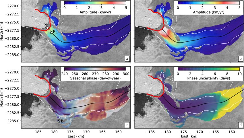
408                                                                              B. Riel et al.: Time-dependent Jakobshavn

   For the past few decades, continental-scale observations      amplification was an increase in the average ice velocity
of ice motion have been derived from the complementary           from 2012 to 2016. Both of these signals have been hypothe-
use of spaceborne optical imagery and synthetic aperture         sized to be driven primarily by changes in the position of the
radar (SAR) data (Scambos et al., 1992; Goldstein et al.,        terminus (Joughin et al., 2012; Bondzio et al., 2017). Start-
1993; Joughin et al., 1998; Rignot et al., 2011; Gardner         ing in winter 2016, this trend reversed: average ice velocities
et al., 2018; Joughin et al., 2018). By comparing optical im-    decreased over the course of 3 years while the seasonal vari-
ages acquired at different times over a common area, sur-        ations decreased in amplitude (Joughin et al., 2018; Khazen-
face deformation can be quantified using feature-tracking-       dar et al., 2019; Joughin et al., 2020a). Thus, the complex
based techniques (Luckman and Murray, 2005; Dehecq et al.,       velocity history at Jakobshavn Isbræ over the past decade
2015; Fahnestock et al., 2016; Kääb et al., 2016). Opti-         provides a unique test case for assessing the quality and fea-
cal data from missions such as Landsat 7 and Landsat 8,          sibility of the time series decomposition method presented
which have provided optical data for countless studies of        here. Specifically, the repeated terminus-driven velocity per-
surface deformation, have recently been supplemented with        turbations at multiple timescales admits a new framework for
data from Earth-observing missions like Sentinel-2, as well      investigating the mechanics of glaciers and ice streams.
as modern cubesat constellations (Kääb et al., 2017). While
optical data depend on daylight conditions and cloud-free
weather, SAR data are able to observe Earth’s surface un-        2   Time series analysis methods
der any condition, thus allowing for temporally dense cover-
                                                                 Geodetic time series contain measurements of geophysical
age over many glaciers and ice streams (Rignot, 1996; Rig-
                                                                 processes with variable spatial and temporal scales. Over
not and Kanagaratnam, 2006; Joughin et al., 2012; Lemos
                                                                 glaciers, mesoscale changes in precipitation or climate may
et al., 2018). The last decade has seen the launch of multi-
                                                                 induce slow and widespread changes in ice surface elevation,
ple SAR satellites which has led to the formation of an in-
                                                                 while calving events at glacier termini and thinning of ice
ternational constellation of all-weather Earth-observing plat-
                                                                 shelves can generate traveling waves that propagate upstream
forms that can provide unprecedented spatial and tempo-
                                                                 over a wide range of timescales (Hewitt and Fowler, 2008;
ral resolutions over many areas of interest. At the same
                                                                 Fowler, 2011; Minchew et al., 2017). Many external forc-
time, several researchers have synthesized these multiple
                                                                 ing functions can result in nonlinear variations in internal ice
data sources to consistently produce repeating ice velocity
                                                                 dynamics due to factors like the non-Newtonian viscosity of
products over Greenland, Antarctica, and other dynamic ar-
                                                                 ice, softening of ice in shear margins by viscous dissipation,
eas of the cryosphere (Joughin et al., 2010, 2011; Nagler
                                                                 lubrication of glacier beds due to surface melt, and changes
et al., 2015; Mouginot et al., 2017; Gardner et al., 2019).
                                                                 in gravitational driving stress taking effect (Schoof, 2010;
These products, many of which are publicly available, have
                                                                 Minchew et al., 2018; Meyer and Minchew, 2018). The ef-
simplified access to high-quality velocity observations, al-
                                                                 fects of these processes are often additive and collocated, so
lowing for a new era of rapid assessment and quantification
                                                                 measurements of ice surface velocity and elevation with suf-
of ice motion over the most critical regions.
                                                                 ficient temporal sampling will record the combined effect of
   In this work, we utilize velocity products generated by
                                                                 all processes. Isolating the spatial and temporal signature of
the Greenland Ice Mapping Project (GIMP), which has used
                                                                 each distinct geophysical mechanism is necessary for identi-
data from a variety of satellites and sensors to observe ice
                                                                 fying the appropriate forcing function and inferring physical
sheet change over Greenland since 2000 (Joughin et al.,
                                                                 properties of the glacier.
2018). In particular, we will focus on forming a tempo-
                                                                    In this study, we generalize previous surface velocity time
rally continuous time-dependent velocity dataset over Ser-
                                                                 series methods (Minchew et al., 2017), which were restricted
meq Kujalleq (hereafter referred to as Jakobshavn Isbræ)
                                                                 to sinusoidal variations in time, by modeling temporal varia-
using high-spatial-resolution velocity data generated with
                                                                 tions in surface velocity as a linear combination of reference
the German Aerospace Center (DLR) TerraSAR-X mission
                                                                 functions that resemble typical signals observed in geodetic
(Joughin et al., 2020a). We present a flexible time series de-
                                                                 time series (Hetland et al., 2012; Riel et al., 2014, 2018).
composition method that allows us to isolate short- and long-
                                                                 These reference functions can be non-orthogonal and are
term variations in the velocity data while also allowing for
                                                                 placed in a large dictionary (matrix), G ∈ RM×N , such that
interpolation of velocity changes between observation times
                                                                 the temporal model for a time series at a given location is
throughout the glacier. This method, coupled with the 11 d
                                                                 linear and given as
repeat time for the TerraSAR-X velocities from 2009–2019,
allows us to investigate numerous changes to the flow char-      d = Gm + N (0, Cd ) ,                                       (1)
acteristics of Jakobshavn Isbræ over the past decade. For
example, the seasonal variations in velocity magnitude that      where d ∈ RM×1 is the vector of observations, m ∈ RN×1 is
became more prominent following the disintegration of the        the coefficient vector solution, and Cd ∈ RM×M is the co-
floating ice tongue in 2004 experienced further amplification    variance matrix corresponding to zero-mean Gaussian obser-
in 2012 (Joughin et al., 2012). Coincident with the seasonal     vation errors N (0, Cd ). Therefore, each reference function

The Cryosphere, 15, 407–429, 2021                                                     https://doi.org/10.5194/tc-15-407-2021
B. Riel et al.: Time-dependent Jakobshavn                                                                                         409

is evaluated over the entire time span of the time series and         plex, sub-annual behavior in the time series data. On the
placed into the columns of G. An important advantage of               other hand, time-integrated B-splines, which exhibit slow-
using a linear model is the ability to evaluate the reference         step behavior at particular timescales (similar to the sigmoid
functions (and thus construct G) at any arbitrary time, which         function), are useful for modeling transient variations. In this
provides a natural way to assimilate time series with missing         work, we define transient signals as any signal that is non-
or irregularly spaced data. Additionally, linear models facili-       steady and non-periodic, which encompasses both rapid tran-
tate the use of powerful and efficient linear regression inverse      sients (e.g., speedup following a calving event) and longer-
methods to solve for the coefficients in m (Tarantola, 2005).         term transients (e.g., multi-year increases in velocity due to
   The dictionary G can contain any combination of func-              long-term changes in air temperatures). This spectrum of be-
tions that collectively capture the observable temporal varia-        havior can be comprehensively reconstructed through a com-
tions. Thus, the inverse problem for m is often ill-posed be-         bination of Bi -splines of different timescales and onset times.
cause the dictionary G can be overcomplete, with many more            For the Jakobshavn Isbræ data analyzed here, we target only
reference functions (columns) than observations (rows).               longer-term transient signals by including Bi -splines with du-
Therefore, we use regularized least squares to obtain an              rations > 1 year in G. Notationally, the partitioning of the
estimate m̂ that minimizes a cost function containing the             design matrix can be represented as G = [GS , GT ], where
data residual and regularization terms, such that (Riel et al.,       GS ∈ RM×NS is the submatrix containing NS B-splines for
2014, 2018)                                                           modeling seasonal signals and GT ∈ RM×NT contains NT Bi -
                n                                      o              splines for modeling transient signals. The regularized least-
m̂ = argminm kd − Gmk2Cd + mT C−1      m m + λkmk1 ,         (2)      squares approach in Eq. (2) thus simultaneously estimates
                                                                      the coefficients for each submatrix such that m̂ = [m̂S ; m̂T ],
where k · kCd denotes the Euclidean or `2 norm that accounts          where m̂S ∈ RNS ×1 and m̂T ∈ RNT ×1 . Simultaneous estima-
for noise in the observations via the data covariance ma-             tion of seasonal and transient signals allows for underlying
trix Cd , Cm ∈ RM×M is a prior covariance matrix that rep-            tradeoffs between the two signal classes to be maximally re-
resents expected statistics of the coefficients (i.e., a priori in-   solved by the full time span of the time series.
formation), and the final term λkmk1 is an `1 -norm term that            To encourage seasonal coherency of the B-spline coeffi-
encourages a sparse number of non-zero coefficients. The              cients, we construct Cm in Eq. (2) such that the B-splines
function in curly brackets in Eq. (2) is a convex cost func-          co-vary with other B-splines that share the same centroid
tion, which provides a solution that is guaranteed to be glob-        time within any given year. The covariance strengths are con-
ally optimal. Implementation and the procedure for solving            structed to decay exponentially in time. The flexibility in rep-
Eq. (2) for m̂ is detailed by Riel et al. (2014).                     resenting potentially complex temporal variations afforded
   The coefficient λ in Eq. (2) is a penalty parameter con-           by this approach avoids the severe limitations of using a sin-
trolling the strength of the sparsity-inducing regularization.        gle or small subset of sinusoidal variations (e.g., Minchew
Schemes for choosing values of λ based on the number of               et al., 2017) and allows for a framework of transient and peri-
data available and the desired smoothness of the solution are         odic variations that readily admit physical interpretation. The
discussed by Riel et al. (2014). In practice, the `1 -norm reg-       interpretability of the resulting posterior model m̂ (which in
ularization can be applied to a subset of m, which is assumed         this study primarily represents surface flow speeds) in terms
to be sparse, and depending on the reference functions in the         of external drivers and intrinsic dynamics of the glacier is
dictionary that correspond to this subset, fewer non-zero co-         a marked advantage of our approach over time series ap-
efficients may result in a smoother time series reconstruction.       proaches based on singular-value decomposition (e.g., Sam-
This regularization approach results in a compact representa-         sonov, 2019). This advantage is amplified when using the
tion for reconstructed signals, which can aid in determining          sparse-regularization techniques to constrain the timing, du-
the dominant timescales and onset times captured in the data          ration, and amplitude of transient events that are superim-
while potentially improving detection of signals with a lower         posed on periodic variations, as we describe in this study.
signal-to-noise ratio (SNR).                                          Importantly, the framework described by Eq. (2) also enables
   In this study, we use a combination of third-order B-              quantification of the formal uncertainty estimates in the in-
splines and time-integrated B-splines (Bi -splines) to popu-          ferred time series (i.e., posterior model m̂).
late the columns of G (Hetland et al., 2012; Riel et al., 2014).         Uncertainties for the estimated model coefficients can be
Third-order B-splines are suitable for modeling seasonal sig-         formally quantified by combining observational uncertain-
nals with potential year-to-year variations in amplitude, as is       ties contained in the data covariance matrix Cd with the dic-
observed in the ice surface velocity and elevation at Jakob-          tionary G and prior covariance matrix Cm (Tarantola, 2005;
shavn Isbræ (Joughin et al., 2010, 2018). To that end, we con-        Bishop, 2006):
struct B-splines with effective durations (full width at half                              −1
maximum) of 3 months, spaced 0.2 years apart such that the            C̃m = GT C−1 G + C −1
                                                                                                ,                                 (3)
                                                                                d        m
center times of the B-splines repeat each year. This choice
of timescale and spacing allows for reconstruction of com-

https://doi.org/10.5194/tc-15-407-2021                                                        The Cryosphere, 15, 407–429, 2021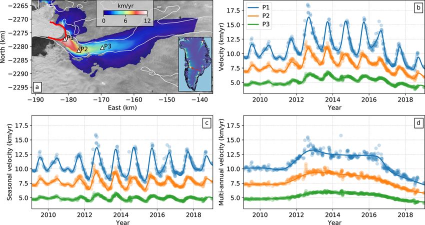
410                                                                                B. Riel et al.: Time-dependent Jakobshavn

where C̃m is the posterior model covariance matrix. Lower          the raw remote sensing data were processed to individual
coefficient uncertainties can thus be obtained by a combina-       time-stamped fields and made publicly available through dif-
tion of reduced data noise and lower prior uncertainties in        ferent projects and publications. In this section, we briefly
those coefficients. Similarly, the posterior covariance matrix     describe these datasets.
of the reconstructed time series can be formally computed as
(Tarantola, 2005; Bishop, 2006)                                    3.1   Surface velocity data

C̃d = GC̃m GT .                                             (4)    The Greenland Ice Mapping Project (GIMP) produces com-
                                                                   prehensive horizontal ice surface velocity time series for
In general, the structure of G, in particular the non-             the Greenland Ice Sheet using a variety of satellites and
orthogonality of the included reference functions, will have a     sensors (Joughin et al., 2010, 2018, 2020a). These data al-
strong effect on the covariances between different model co-       low for widespread observations of glacier velocity varia-
efficients and time epochs via the off-diagonal values in the      tions with increasing temporal resolution as more data from
matrices C̃m and C̃d , respectively. Properly quantifying these    more sensors became available. Over select glaciers like
uncertainties and covariances is critical for any subsequent       Jakobshavn Isbræ, 11 d and monthly repeat TerraSAR-X–
interpretation or analyses using the modeled time series.          TanDEM-X (TSX) SAR pairs for both ascending and de-
   After using Eq. (2) to estimate m̂ for a given data time se-    scending orbits are available and provide a much higher tem-
ries d, the seasonal and transient signals can be reconstructed    poral resolution than is available on many other glaciers. The
as                                                                 GIMP velocity maps are formed using speckle-tracking tech-
                                                                   niques on each SAR pair (Joughin, 2002). Speckle tracking
d̂ S = GS m̂S ,
                                                                   is generally more robust to large-scale displacements than
d̂ T = GT m̂T ,                                             (5)    standard interferometric methods and allows for uncertainty
                                                                   quantification through estimates of the statistics of correla-
where d̂ S and d̂ T are the reconstructed seasonal and transient   tion measurements. These formal errors are provided with
signals, respectively. Correspondingly, we can use these re-       the GIMP velocity fields.
constructed signals to detrend the data, e.g.,                        In this work, we use 555 GIMP horizontal velocity fields
                                                                   generated from TSX data covering the period 2009–2019.
d S = d − d̂ T ,                                                   The velocity fields are provided with 100 m grid spacing, and
                                                                   the short repeat times allow for mostly complete spatial cov-
d T = d − d̂ S .                                            (6)
                                                                   erage of Jakobshavn Isbræ due to the high number of coher-
                                                                   ent surface features facilitating a high SNR for the speckle-
Throughout this paper, references to short-term, seasonal ve-
                                                                   tracking techniques. During the course of this work, we dis-
locity variations refer to d̂ S while references to longer-term,
                                                                   covered systematic discrepancies in velocity measurements
multi-annual velocity variations refer to d̂ T .
                                                                   between SAR pairs collected from ascending and descending
   In some cases it may be desirable to enforce spatial co-
                                                                   orbits at the same geographic location and approximately the
herency when solving for m̂ to reduce the influence of data
                                                                   same time. These discrepancies are generally limited to the
noise on m̂ (Hetland et al., 2012; Riel et al., 2014; Minchew
                                                                   shear margins of the glacier and cluster in areas much smaller
et al., 2015). Examples of such cases involve low-amplitude
                                                                   than the glacier. To improve the overall quality of the time se-
signals with spatial wavelengths longer than a single data
                                                                   ries, we masked out areas where the velocities collected from
pixel and, more generally, cases where the data have low
                                                                   near-coincident ascending and descending orbits differed by
SNR values. The software made available with this study al-
                                                                   more than 250 m yr−1 .
lows the user to enforce spatial coherency (see Riel et al.,
                                                                      To extend the velocity time series, we include monthly
2018), but for the velocity and elevation time-dependent
                                                                   GIMP velocity maps derived from optical Landsat imagery
datasets used in this study, we do not enforce spatial coher-
                                                                   for the years 2004–2009 (Jeong et al., 2017). This longer
ence between neighboring pixels because doing so can be
                                                                   time series allows us to compare long-term trends in surface
computationally expensive and is unnecessary in our case.
                                                                   velocity to long-term changes in the glacier terminus posi-
Instead, we solve for m̂ for each pixel independently and jus-
                                                                   tion. The optical velocity maps are provided at 100 m grid
tify this decision based on the fact that the SNR is generally
                                                                   spacing on a grid that is not aligned with the TSX veloc-
high over Jakobshavn Isbræ, reducing the need for spatial co-
                                                                   ity maps. Thus, we resampled the Landsat-derived velocity
herency in the inversion process.
                                                                   fields to the same grid as the TSX velocity fields.

3     Data                                                         3.2   Surface elevation data

Data used in this study provide information on the time-           Ice surface elevation will rise and fall in response to vari-
dependent surface velocity and elevation fields. In both cases,    ations in mass balance and ice flow. While time-dependent

The Cryosphere, 15, 407–429, 2021                                                       https://doi.org/10.5194/tc-15-407-2021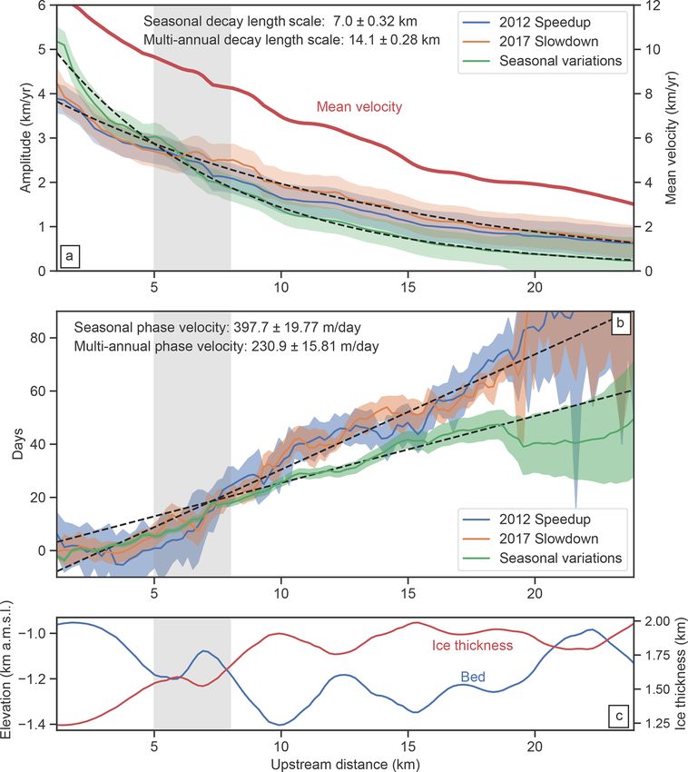
B. Riel et al.: Time-dependent Jakobshavn                                                                                     411

measurements of surface elevation are generally available         position for the calving front to be a feature in the bedrock to-
at a lower temporal resolution than measurements of ve-           pography with reported dynamical implications for flow vari-
locity, the increased availability of optical imaging satel-      ations on Jakobshavn Isbræ. Cassotto et al. (2019) suggested
lites and robustness of photogrammetry techniques has al-         that the acceleration in velocities in 2012 corresponded to
lowed for the generation of time-dependent digital-elevation-     a retreat of the calving front passed a narrow, shallow por-
model (DEM) strips at sub-annual epochs. Here, we use pub-        tion of the bed topography, which acts as a pinning point
licly available DEMs from ArcticDEM and the Oceans Melt-          that facilitates higher extensional and lateral shear stresses
ing Greenland (OMG) mission.                                      relative to the wider and deeper basin upstream (Morlighem
   The ArcticDEM initiative automatically produces 2 m res-       et al., 2017). This suggestion is a generalization of the often-
olution DEM strips over all the land area north of 60◦ lat-       mentioned process of retreat of the calving front into an
itude using stereo auto-correlation techniques (Porter et al.,    overdeepened basin (e.g., Nick et al., 2009; Joughin et al.,
2018). We use DEMs generated from optical data collected          2012) and has been reproduced in three-dimensional mod-
over Jakobshavn Isbræ from 2010 to 2017. The geographical         els incorporating detailed bed topography (e.g., Morlighem
extent of the strips and their associated acquisition times are   et al., 2016). We therefore generate a time series of the inter-
irregular, so we interpolate the strips onto a uniform spatial    section of the calving front with the glacier centerline, ref-
grid using inverse distance weighting while using nearest-        erenced to the downstream position of the aforementioned
neighbor interpolation in time to sample the strips onto a uni-   shallow bed location. To reduce time series noise and facili-
form temporal grid.                                               tate comparison with the velocity time series, we again apply
   Because ArcticDEM data are available from 2010 to 2017,        our linear least-squares method to represent the front time
a timescale shorter than the GIMP surface velocity data, we       series as a combination of B-splines for short-term, seasonal
augment the surface elevation time series with DEMs pro-          signals and integrated B-splines for long-term transient sig-
duced annually by the Oceans Melting Greenland (OMG)              nals. Since the absolute position of the front relative to the
mission in March 2017–March 2019. The OMG DEMs were               shallow bed location is important, we do not isolate the front
constructed with Ka-band single-pass SAR interferometry           seasonal (short-term) signal from the time series in the sub-
from the Glacier and Ice Surface Topography Interferom-           sequent analysis.
eter (GLISTIN-A) instrument, providing high-precision (<
50 cm) elevation maps over 10–12 km wide swaths over var-
ious marine-terminating glaciers in Greenland (OMG Mis-           4     Results
sion, 2016). These interferometric products were processed
to an intrinsic resolution of 3 m and then georegistered to a     Hereafter, we focus on applying the time series analysis
ground spacing of approximately 3 m. For comparison with          methods presented in Sect. 2 to analyze and decompose
velocity data, both ArcticDEM and OMG DEMs were re-               the observed time-dependent velocity magnitude (speed) and
sampled to a grid spacing of 100 m.                               surface elevation fields summarized in Sect. 3 into sub-
                                                                  annual (primarily seasonal) and multi-annual transient varia-
3.3   Calving front positions                                     tions. Our focus is on quantifying the rates and distances over
                                                                  which stress perturbations of various frequencies propagate
To elucidate the connection between observed changes in the       through Jakobshavn Isbræ. We use only the time-dependent
terminus position and observed variations in ice surface ve-      flow speeds because Jakobshavn Isbræ flows along a deep,
locity and elevation, we use calving front positions from a       narrow channel in the underlying bed, which leads to tem-
variety of sources. The main source are calving front posi-       porally consistent velocity unit vectors throughout the obser-
tions automatically determined from TSX images acquired           vation period. Future work will be aimed at adding multidi-
from 2009 to 2015 (Zhang et al., 2019). We supplement these       mensional capability to the time series analysis methods we
data with calving front locations provided by the Green-          introduce in this study. Before proceeding to the analysis of
land Ice Sheet Climate Change Initiative (CCI) from 2000          the time-dependent velocity fields, we note for completeness
to 2016, which were computed using manual digitization of         that we observe magnitudes and spatial patterns of mean flow
ERS, Sentinel-1, and Landsat imagery (ESA, 2016). We fur-         speed that are consistent with previous studies, with the high-
ther supplement the data with our own manual digitization of      est speeds near the terminus decaying quasi-exponentially
the calving front from TerraSAR-X images, skipping months         with upstream distance (Fig. 1a and b; Movie S1; Riel, 2020).
where the front position is not clear (Joughin et al., 2020a).    We also note that for all time series model fits presented here,
The upper bound of horizontal position errors for these data      the output sampling period is approximately 4 d.
is approximately 200 m, which indicates sufficient accuracy
for the qualitative comparison with ice velocities performed      4.1    Seasonal variations in surface velocity
here.
   To develop a time series of calving front positions for com-   The reconstructed velocity time series demonstrates the abil-
parison with our velocity fields, we first choose the reference   ity of our flexible method to smoothly interpolate the velocity

https://doi.org/10.5194/tc-15-407-2021                                                     The Cryosphere, 15, 407–429, 2021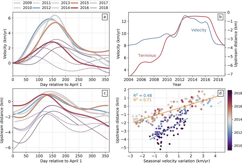
412                                                                                      B. Riel et al.: Time-dependent Jakobshavn

Figure 1. Sermeq Kujalleq (Jakobshavn Isbræ) mean velocity field and select velocity time series. (a) Mean velocity between 2009 and 2019
in Polar Stereographic North (EPSG:3413) coordinates. The background image is a Landsat 8 image acquired in August 2017. White lines
correspond to the bed topography (BedMachine V3) at sea level, and the red line indicates the winter 2017 terminus position (for all
subsequent map figures). White triangles indicate the points P1–P3 from which data shown in (b–d) are taken. Inset shows (with red arrow)
the approximate study area within Greenland with mean velocities from Joughin et al. (2011). (b) Time-dependent speed at points P1–P3.
(c) Short-term velocity time series showing predominantly seasonal variations. For each time series, mean velocities for 2009–2019 have
been added as offsets for visual clarity. (d) Long-term velocity time series showing the 2012 speedup and 2017 slowdown. In (b–d), solid
lines show our model results while dots indicate (b) observed speeds or (c, d) detrended observations. The detrended short-term observations
in (c) are the observed speeds minus the estimated integrated B-splines. The detrended long-term observations in (d) are the observed speeds
minus the estimated seasonal B-splines.

data in time in a manner that preserves the seasonal varia-             terline transect shown in Fig. 4a. This representation allows
tions. In particular, the use of temporally coherent B-splines          for an intuitive visualization of spatiotemporal variations in
to model seasonal variations allows for reconstruction of sev-          the surface velocity fields and, most relevant for this study,
eral summer speedup events where data happen to be more                 the propagation of velocity variations through the glacier in
sparse for certain years (Fig. 1). By applying Eq. (5) to de-           time. Our analysis focuses on this propagation by treating
compose the velocity magnitude time series into seasonal and            velocity variations as traveling waves with quantifiable at-
transient components (d̂ S and d̂ T , respectively), we show that       tenuation and propagation rates. To aid in this discussion, we
short-term velocity variations on Jakobshavn Isbræ are dom-             have provided a visual representation of the upstream prop-
inated by the seasonal cycle of summer speedup and winter               agation rate in Fig. 2 using the solid and dashed black lines.
slowdown. In this section, we focus on these seasonal varia-            The angle between the two lines represents the phase veloc-
tions, leaving discussion of the multi-annual transient varia-          ity cp , an important concept in this study that is defined as the
tions for the next section.                                             speed at which the phase of a wave of a given frequency ω
   The flexibility of the B-spline representation for the sea-          travels. Thus, cp = ω/kr , where kr is the real component of
sonal time series allows us to quantify the change in the am-           the angular wavenumber.
plitude of summer speedup from year to year and at each                    The results shown in Figs. 1c and 2a indicate that the am-
point on the glacier. In Figs. 1 and 2 we show these vari-              plitudes of seasonal velocity variations are largest near the
ations in two different views to aid in interpretation of the           terminus and decay as a function of upstream distance. By
results. Figure 1a and b represent a classical view of spa-             extracting a centerline transect of amplitude (averaged over
tiotemporal variations in surface velocity, with a map of sec-          all observed seasons) as a function of distance, we estimate
ular velocity (Fig. 1a) and time series of select points on the         an attenuation (or e-folding) length scale of approximately
glacier (Fig. 1b). Figure 1c shows, for the same points on              7 ± 0.3 km for all observed seasonal variations (Fig. 3a),
the glacier, the seasonal variations, which are the total signal        which implies that large-amplitude velocity variations near
shown in Fig. 1b less the inferred multi-year trends discussed          the terminus position are observable at farther-upstream dis-
in the next section. In Fig. 2, we present a space–time plot for        tances relative to smaller-amplitude variations. This effect
the (a) seasonal and (b) multi-year variations along the cen-           can be observed by comparing in map view seasonal velocity

The Cryosphere, 15, 407–429, 2021                                                              https://doi.org/10.5194/tc-15-407-2021
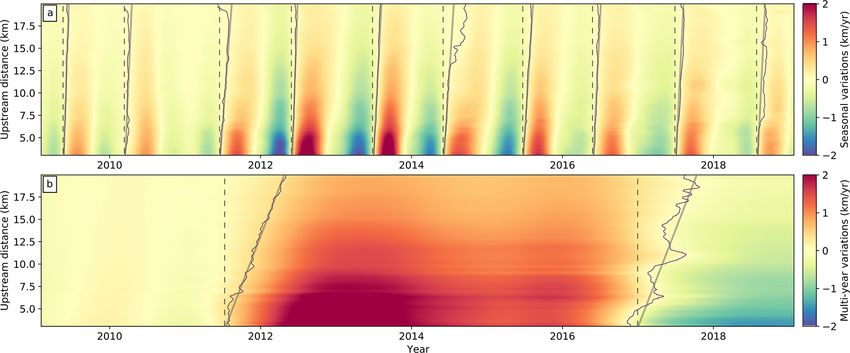
B. Riel et al.: Time-dependent Jakobshavn                                                                                                  413

Figure 2. Temporal evolution of glacier flow variations along a centerline segment for decomposed seasonal (a) and multi-year (b) signals.
The centerline trace is shown in map view in Fig. 4, and distance values here are measured upstream along the centerline from the winter 2017
terminus position. Thin black lines correspond to contours of zero-velocity variation at the initiation of each signal – summer speedups for (a)
and 2012 speedup and 2017 slowdown for (b). Solid gray lines approximately follow the zero-velocity contours and indicate the leading edges
of propagating velocity variations. Vertical dashed gray lines indicate onset times for the propagating wave initiating at the terminus and are
equivalent to the propagation path for a wave with infinite propagation speed. The tangent of the angle between solid and dashed gray lines
is the phase velocity averaged over the observable propagation distance. The marked difference in phase velocities between the seasonal and
multi-year signals indicates (frequency) dispersion.

variations for years when the amplitudes are markedly differ-             rigidity during the course of the seasonal cycle (Joughin
ent (Fig. 4a and b). For the years 2009–2011 and 2017–2018,               et al., 2020a). Nevertheless, the spatial pattern of relative tim-
peak amplitudes of seasonal velocity variations did not ex-               ing in the upstream direction from the terminus is broadly
ceed 3 km yr−1 , whereas for the years 2012–2015 (the period              consistent even among years with large differences in mean
with the fastest glacier flow speeds in our observations) the             velocities, which indicates a common mechanism for the sea-
highest amplitudes exceed 6 km yr−1 . Thus, there is a clear              sonal cycle (Fig. 2a). As expected for marine-terminating
correlation between mean flow speed for a given year and                  glaciers like Jakobshavn Isbræ, the timing of the peak sea-
the amplitude of seasonal variations, which we will explore               sonal signal indicates that seasonal variations originate at the
in later sections.                                                        terminus and propagate upstream (Figs. 1c and 2a).
   In addition to attenuation, we are interested in constrain-               To investigate the spatial characteristics of the timing of
ing the rate of propagation of surface velocity variations.               peak velocity, we fit a simple temporal model using a sum
We quantify these variations in terms of phase velocities                 of sinusoids to the velocity data from 2011 to 2019 at each
by constraining the relative timing of peak velocity for dif-             pixel with the estimated long-term signals removed, d S (e.g.,
ferent temporal frequencies. As with amplitude, we present                Fig. 1c), such that
the absolute and relative timing of the velocity variations in                        X
multiple ways to help build a more intuitive framework for                d S = C0 +       [Ci cos (ωi t) + Si sin (ωi t)] ,              (7)
the reader. This presentation follows the same structure as                              i
the amplitude variations discussed in detail above, with a                where ωi is the angular frequency for the ith sinusoid; Ci and
classical view shown in Fig. 1, the space–time diagram in                 Si are the coefficients of the cosine and sine components,
Fig. 2, the mean over all seasons along a centerline transect             respectively; and C0 is a constant offset. After estimating the
in Fig. 3b, and a map view of the relative timing in Fig. 4c              values of Ci and Si , the amplitude and phase (i.e., relative
(with formal uncertainties in timing given in Fig. 4d).                   timing) of each sinusoid can be recovered as
   For seasonal variations in surface velocity, the time of peak
velocity varies slightly from year to year, with the earliest                  q
peaks occurring around mid-August and the latest peaks oc-                ai = Ci2 + Si2 ,                                            (8)
curring around mid-September. The exception to this timing                φi = tan−1 (Ci /Si ) .                                            (9)
is the 2010 speedup which starts earlier in the year and may
have been driven by a combination of warmer air temper-                   While this model cannot accurately reproduce the am-
atures and cooler ocean temperatures influencing mélange                  plitude changes or nonsinusoidal variations (e.g., Joughin

https://doi.org/10.5194/tc-15-407-2021                                                               The Cryosphere, 15, 407–429, 2021
414                                                                                          B. Riel et al.: Time-dependent Jakobshavn

Figure 3. Glacier centerline transects of phase delay and velocity variation amplitude for the seasonal, 2012 speedup, and 2017 slowdown
signals compared to centerline ice thickness and bed depth. (a) Velocity variation amplitude and 1 SD (standard deviation) uncertainties for
the three different signals. The decay length scale (e-folding distance) for the multi-annual signals is roughly twice that of the seasonal signal
(represented by best-fit exponential decay model in dashed black lines). Dark-red line corresponds to the mean velocity magnitude along the
centerline (note the 2× scaling factor for the mean velocity axis). (b) Relative phase delay for the three different signals: seasonal phase delay
– green; 2012 speedup - blue; 2017 slowdown – orange. The upstream centerline distance is with respect to the intersection of the centerline
and the 2017 terminus. For distances greater than 8 km upstream, the phase velocity for the seasonal signal is roughly twice as fast as the
phase velocities for the multi-annual transients (represented by dashed black lines). The shaded areas represent the 1 SD formal uncertainties
for the annual phase (green) and bootstrapped standard deviation for the transients (blue and orange). (c) Centerline ice thickness (red) and
bed depth (blue) using bed data from BedMachine V3 (Morlighem et al., 2017). For all plots, the gray-shaded region represents the upstream
region encompassed by the southern bend.

et al., 2008, 2014), the seasonal phase can be estimated ro-                  The seasonal phase map shows upstream transmission of
bustly with 7 years of data. Note that the years 2009–2010                 velocity perturbations originating at the terminus (Figs. 3b
are excluded in order to avoid introducing biases into the                 and 4c). This propagation occurs rapidly in the first 5 km
phase estimation from differences in onset times of summer                 upstream of the terminus and then slows to a near-constant
speedups. Furthermore, we can compute the formal phase                     phase velocity of 398 ± 20 m d−1 (approximately 146 ±
uncertainties following the procedure outlined in Minchew                  7 km yr−1 ), which is more than an order of magnitude faster
et al. (2017). The estimated seasonal phase is thus equiva-                than the mean flow speed near the terminus. Our estimates of
lent to the mean time of peak seasonal velocity for the 2011–              the phase velocity within the first 5 km upstream of the ter-
2019 period while the phase uncertainty is proportional to the             minus are limited by the temporal resolution of the data, but
formal variance of the mean.                                               by considering the uncertainties in timing, we estimate that

The Cryosphere, 15, 407–429, 2021                                                                  https://doi.org/10.5194/tc-15-407-2021
B. Riel et al.: Time-dependent Jakobshavn                                                                                                415

Figure 4. Seasonal variations in flow speed and timing of peak velocities. (a) Mean seasonal velocity amplitude for the years 2009–2011
and 2017–2018 (years not associated with the increased velocities between 2012 and 2015). Triangular markers indicate comparison points
used in Fig. 7: pinning point (PP) where the bed topography locally narrows and reference point 1.4 km upstream from the 2017 front
position (P1.4 ). (b) Mean seasonal velocity magnitude variation for the years 2012–2015 (2016 excluded due to higher background velocities
at the start of the summer). (c) Mean day of year of peak seasonal velocity (i.e., seasonal phase) for entire observation period. SB indicates
the southern bend referred to in the text. (d) Seasonal phase uncertainty (1σ ). Seasonal amplitudes are measured as the difference between
the summer high and winter low velocities in the short-term time series as shown in Fig. 1c. The highest amplitudes occur at the terminus
and decay exponentially upstream.

the phase velocity in this region must be at least 500 m d−1             that begins in 2012 and a slowdown that begins in late 2016
(182.5 km yr−1 ), or approximately 18 times the local mean               near the terminus, which we refer to as the 2017 slowdown.
glacier flow speed. In the across-flow direction, about 8 km             We present the results for multi-annual variations using the
upstream from the 2017 calving front, the center of the                  same general structure as for the seasonal ones, with the time
glacier reaches its peak velocity earlier than the margins               series view shown in Fig. 1, the space–time diagram in Fig. 2,
by about 15 d, indicating a nonlinear relationship between               along a centerline transect in Fig. 3, and the map view of the
time-dependent lateral shear strain rates and centerline ve-             amplitudes and phase values in Fig. 5.
locity, meaning that the effective width of the shear mar-                  The spatial pattern of the amplitudes of multi-annual ve-
gins (defined here as the centerline velocity divided by the             locity variations is remarkably consistent between the two
maximum shear strain rate) must change over the seasonal                 observed events, with the highest amplitudes at the terminus
cycle. Finally, we note that the phase uncertainty is gener-             and an exponential decay with distance upstream (Figs. 3a
ally lowest in the center of the glacier where amplitudes are            and 5a, b). Notably, the velocity variations induced by these
higher and increases with distance upstream as the ampli-                events have an attenuation (e-folding) length scale of ap-
tudes decay (Fig. 4d), as expected from the formal uncertain-            proximately 14.1 ± 0.3 km, which is about twice the atten-
ties (Minchew et al., 2017).                                             uation length for seasonal variations (Fig. 3a). As a result,
                                                                         we are able to observe multi-annual velocity variations far-
4.2   Multi-year variations in surface velocity                          ther upstream than the seasonal timescale velocity variations
                                                                         (Fig. 2b).
After isolating the long-term signals from the short-term sea-              From the phase delay of the multi-annual signals, we can
sonal signals (i.e., d̂ T ), we can observe clear variations in          see that both the 2012 speedup and 2017 slowdown signals
multi-annual amplitudes at different points along the glacier            originate at the terminus, propagate rapidly along the first
(Figs. 1d and 2b). The temporal density of the velocity time             5 km of the glacier, slow down through the southern bend
series allows us to quantify spatial variations in the amplitude         between 5–8 km, and propagate upstream from 8–20 km at a
and timing of the positive and negative multi-annual trends,             generally consistent phase velocity (Figs. 3 and 5c, d). Be-
much like we did with seasonal velocity variations in the pre-           yond 20 km upstream, the amplitudes for the velocity varia-
vious sections. We observe two events in the data: a speedup

https://doi.org/10.5194/tc-15-407-2021                                                              The Cryosphere, 15, 407–429, 2021
416 B. Riel et al.: Time-dependent Jakobshavn
Figure 5. Velocity variation amplitude and phase delay maps for 2012 transient speedup (a, c) and 2017 transient slowdown (b, d). In (c),
SB indicates the southern bend referred to in the text. Red line indicates winter 2017 terminus position. In addition to the spatial distribution
of phase delay and amplitude being consistent for the two events, these transient phase delays show strong similarities with the seasonal
phase delay. However, the transient amplitudes show farther-upstream propagation than the seasonal amplitudes.
tions become too low to reliably estimate the timing of ar- 4.3 Multi-year variations in surface elevation
rival of the transient signals (Fig. 5d). The phase velocity be-
tween 8 and 20 km upstream is approximately 231±16 m d−1
(84 ± 6 km yr−1 ), which is a little more than half of the phase Ice surface elevation varies in response to changes in snow
velocity for the seasonal signal and roughly 7 times the mean accumulation and melt (the sum of which constitutes the
flow speed near the terminus. For glaciers where ice flow surface mass balance; SMB), firn compaction (Herron and
is dominated by basal sliding, phase velocity is expected to Langway, 1980; Huss, 2013; Meyer et al., 2020), and dy-
scale with the square root of ice thickness and basal shear namic thinning (thickening) in response to increases (de-
traction (Rosier et al., 2014), which is roughly consistent creases) in the flux divergence of the ice. The interplay
with the increase in phase velocity and ice thickness around between observed elevation and velocity changes at differ-
8 km upstream, although more work is needed to establish ent temporal and spatial scales can thus yield insight into
concrete connections. As with the observed seasonal vari- the mechanisms driving longer-term elevation and velocity
ations, the phase velocity in the first 5 km upstream of the changes.
terminus is at the limit of the temporal resolution of the For this work, the temporal sampling of the available ele-
data with a lower bound on the phase velocity of at least vation data (ArcticDEM and OMG DEMs) permits only the
500 m d−1 (182.5 km yr−1 ), or approximately 18 times the comparison of longer-term variations in velocity and eleva-
mean glacier flow speed in this region. While the slowdown tion. Thus, we compare the long-term velocity and elevation
in wave propagation in the southern bend is coincident with changes for four successive time periods of length 2.2 years:
a local high in the bed topography, more work is needed to (1) June 2010 to September 2012, (2) September 2012–
evaluate whether the topographic effect is the dominant con- November 2014, (3) November 2014–January 2017, and
trol on wave propagation. The apparent slowdown may also (4) January 2017 to March 2019 (Fig. 6).
be an artifact of numerical errors caused by tracking of peak Within the main trunk of the glacier, we observe a clear
acceleration and deceleration rather than a multi-year aver- association between the 2012 speedup and lowering of the
age of the sinusoidal phase as for the seasonal signal. Nev- ice surface due to dynamic thinning, whereas on the slower
ertheless, the consistency in the spatial distribution of peak ice, thinning is more diffuse and occurs at a lower rate. A
timing and amplitude reinforces the notion that a common comparison of time series for points on and off the glacier
physical mechanism is responsible for multi-year and sea- (Fig. S1 in the Supplement) suggests that much of the ice in
sonal velocity variations. the surrounding areas has been lowering since before the ob-
servation period. In these areas, thinning has been attributed
to inland diffusion of steepening surface slopes following
The Cryosphere, 15, 407–429, 2021 https://doi.org/10.5194/tc-15-407-2021B. Riel et al.: Time-dependent Jakobshavn 417
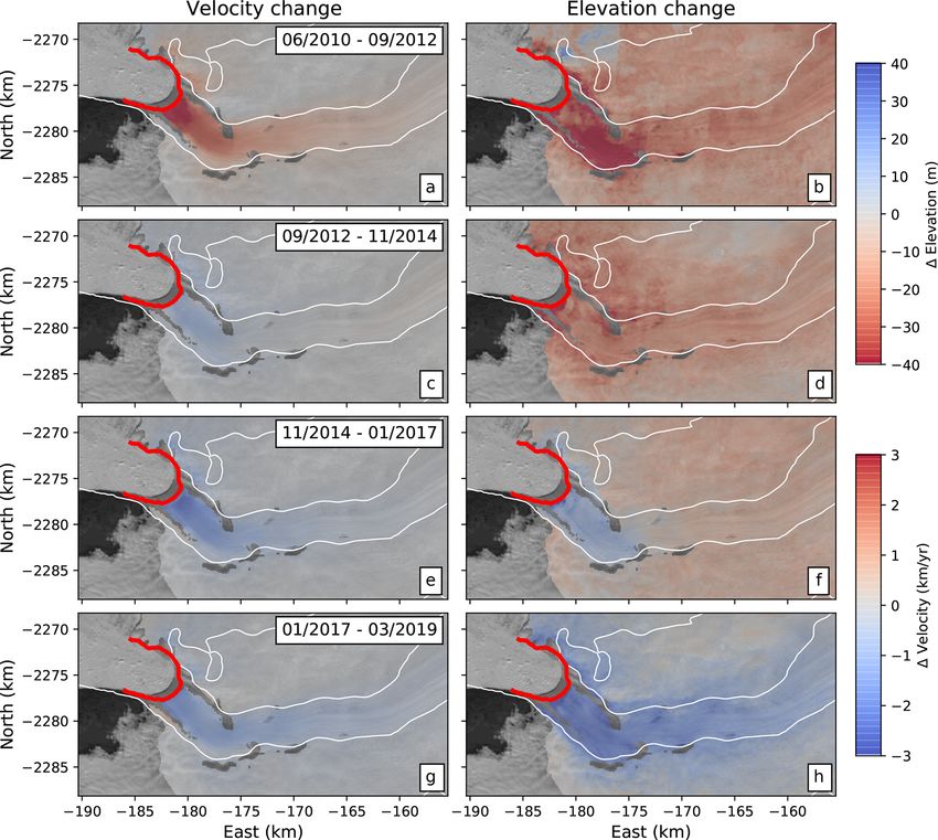
Figure 6. Long-term velocity and ice surface elevation changes for successive time periods of 2.2 years. (a, b) June 2010 to September 2012:
the glacier is accelerating (positive velocity anomaly) and thinning (negative elevation anomaly), with higher rates of thinning within the
glacier. (c, d) September 2012 to November 2014: velocities show slight deceleration while the ice surface lowers over a wider area, indicating
persistent surface melt. (e, f) November 2014 to January 2017: this time period contains the initiation of the 2017 slowdown, which is
associated with ice thickening in the main trunk of the glacier. Note the continuing surface melt signal indicated by lowering distal to the
glacier. (g, h) January 2017 to March 2019: slight decrease in glacier flow speed and more widespread increase in ice surface elevations due
to positive SMB can be seen.
speedup and thinning of the fast-flowing trunk in 2004 in lower than they were in 2010, particularly for the ice outside
response to disintegration of the ice tongue (Krabill et al., of the main trunk of the glacier (Fig. S1).
2004; Joughin et al., 2008). The widespread lowering of the
ice surface persists even during the slight deceleration of ve- 4.4 Calving front forcing
locities over the glacier from 2012 to 2015 (Fig. 6c and d).
During these years, the ice surface has likely adjusted to The position of the calving front has been reported to be the
the initial speedup in 2012, leading to a reduction in driv- dominant factor influencing ice dynamics for Jakobshavn Is-
ing stress and velocities. The 2017 slowdown is coincident bræ over observable, particularly seasonal, timescales (Nick
with thickening of the ice on the main trunk of the glacier et al., 2009; Joughin et al., 2012; Podrasky et al., 2012, 2014;
while the inland ice continues thinning (Joughin et al., 2018; Bondzio et al., 2017). The position of the calving front
Khazendar et al., 2019; Joughin et al., 2020a). From 2017 is heavily influenced by bed topography (Xu et al., 2013;
onwards, we observe more widespread thickening of the ice Morlighem et al., 2016), local ocean temperatures that in-
as the glacier velocities continued to decrease. Despite the fluence subaqueous melting of the terminus (Holland et al.,
recent thickening trend, elevation values are still measurably 2008; Khazendar et al., 2019), and changes in mélange rigid-
ity (Joughin et al., 2008; Cassotto et al., 2015; Robel, 2017;
Xie et al., 2019; Joughin et al., 2020a). Changes in the calv-
https://doi.org/10.5194/tc-15-407-2021 The Cryosphere, 15, 407–429, 2021418 B. Riel et al.: Time-dependent Jakobshavn Figure 7. Comparison between time series of observed terminus positions and ice velocities at various timescales. (a) Seasonal ice centerline velocity at a point 1.4 km upstream from the reference 2017 terminus position (location shown in Fig. 4). Speeds are shown on an annual timescale (referenced to 1 April) and are plotted relative to the speed on 1 April of the respective year. Line colors correspond to the color map in (d), and bold lines correspond to the years 2012–2016 where strong amplification of the seasonal variations is observed (Fig. 1). (b) Long-term ice velocity and terminus position. Velocities are extracted from the same point as in (a). Terminus positions are measured at the intersection of the time-varying calving front with the glacier centerline and are referenced to the position of the shallow pinning point highlighted by Cassotto et al. (2019). (c) Seasonal variations in terminus position with line colors and widths corresponding to lines in (a). (d) Correlation between terminus position and seasonal velocity (i.e., d̂S ) at the same location as in (a) and (b). Here, the points have been grouped into two temporal clusters: July 2011–January 2017 (diamonds) and all other times (circles), with the former time frame defined by the period when maximum seasonal retreat of the terminus position took it behind the reference pinning point. Thus, the scaling relationship between terminus position and velocities changes depending on whether the terminus has retreated beyond the pinning point. The text colors for the R 2 values correspond to the trend-line colors, while the point colors in (d) correspond to line colors in (a) and (b). ing front driven by iceberg calving can reduce back stresses meltwater in the summer melt season. While the role of basal upstream of the new calving front, allowing ice near the ter- lubrication has been shown to affect the seasonal cycle on minus to accelerate and subsequently thin. Local thinning of certain glaciers (e.g., Howat et al., 2010; Bevan et al., 2015), the ice steepens the surface slope, thereby increasing grav- the magnitude and timescale of the influence of basal lubri- itational driving stress and causing further acceleration and cation on the velocities in Jakobshavn Isbræ remains unre- thinning (Joughin et al., 2012). For glaciers where the calv- solved. ing front is located on a retrograde bed, the thinning-induced Consistent with earlier work (e.g., Joughin et al., 2012; retreat of the terminus corresponds to increasing terminus ice Cassotto et al., 2019) but using our method to decompose thickness, which further increases the driving stress (Joughin velocity time series into short- and long-term variations, we et al., 2020a). The redistribution of mass during dynamic observe strong correlations between variations in ice velocity thinning propagates upstream as traveling waves, with phase and variations in the front at both seasonal and long-term velocities and attenuation length scales that we constrain us- timescales (Fig. 7). ing the methodology presented in this study. The thinning The timing of the maximum retreat for a given year is of the ice surface throughout the glacier is hypothesized to closely associated with the timing of peak seasonal ice ve- cause a further, indirect enhancement of velocities by causing locity within a few kilometers of the front position. Here, a reduction in overburden pressure (weight of the ice column we choose a point approximately 1.4 km upstream of the per unit area), which influences the response of the glacier 2017 terminus in order to maximize data availability close to to processes such as basal lubrication by drainage of surface the front position for all years. For the 4 years associated with The Cryosphere, 15, 407–429, 2021 https://doi.org/10.5194/tc-15-407-2021
B. Riel et al.: Time-dependent Jakobshavn                                                                                      419

increased seasonal velocity amplitudes (2012–2015) during          other hand coincided with a 2 km retreat of the calving front
the summer, the calving front retreats past a narrow sec-          (Fig. 7b).
tion in the bed referenced by Cassotto et al. (2019) (defined
as our reference position for the terminus position time se-
ries and shown in Fig. S2) into the wider and deeper basin         5     Discussion
(values > 0 in Fig. 7c), which supports previous hypothe-
ses that even subtle bed constrictions in the fjord can lead       Decomposition of the time-dependent velocity and surface
to large increases in ice velocity in response to terminus re-     elevation fields into distinct temporal scales reveals a repeat-
treat when ice elevations are near flotation heights (Cassotto     ing pattern on Jakobshavn Isbræ where velocity and surface
et al., 2019). In 2016, the calving front also retreats past the   elevation variations originate at the terminus. The coinci-
same pinning point, but the seasonal velocities do not reach       dence of speedup and slowdown of the glacier with thinning
the same peak as in the previous 4 years. In fact, in 2016,        and thickening, respectively, suggests a dynamic origin of the
the calving front starts the summer melt season in a more          physical mechanism generating these variations. Prior stud-
retreated position, which is a consequence of the front not        ies have proposed that this mechanism is primarily character-
sufficiently advancing in 2015 and prematurely retreating in       ized by a reduction in back stress at the terminus following
December of that year. Thus, while the seasonal amplitude          a series of calving events, causing ice acceleration and in-
in 2016 is less than in the previous 4 years, the absolute         creased driving stresses to propagate upstream which results
velocities are still high (Fig. 1c). For the years 2009–2011       in the observed high correlation between calving front posi-
and 2017–2018, the calving front does not retreat past the         tion and velocity variations (e.g., Nick et al., 2009; Joughin
pinning point, which results in seasonal velocity variations       et al., 2012; Bondzio et al., 2017). In this section, we detail
with markedly smaller amplitudes.                                  the observed wave phenomena, introduce the proposition that
   Following Lemos et al. (2018), we compute the correla-          the observed traveling waves are kinematic waves, and dis-
tion between the measured calving front position (relative to      cuss possible paths for future development of observational
the reference pinning point) and short-term velocities for the     methods that will enable progression toward robust and effi-
same point 1.4 km upstream of the 2017 terminus (Fig. 7d).         cient techniques for fusing remote sensing data from multiple
The change in the velocity response to front variations be-        sources and using in situ observations as prior information to
tween 2012 and 2015 can be clearly seen as a distinct cluster      constrain the inversions.
as compared to the other years in the observation period. For
this 4-year period, a linear regression yields a coefficient of    5.1    Wave phenomena
determination (R 2 ) of 0.71 with seasonal velocities scaled by
2.2 km yr−1 per kilometer of front retreat. For the other years,   Our results indicate that velocity variations initiating at the
the regression results in an R 2 of 0.48 with a scale factor of    terminus of Jakobshavn Isbræ propagate upstream as trav-
1.2 km yr−1 per kilometer of front retreat. Thus, from 2012        eling waves with frequency-dependent propagation speeds
to 2015, the velocity response is more strongly correlated         (phase velocities) and attenuation length scales. To our
with front position with larger peak-to-peak variations than       knowledge, ours are the first results to explicitly quantify
for the other years, presumably due to the retreat of the front    wave propagation at seasonal and multi-annual timescales
past the reference pinning point described by Cassotto et al.      using remote sensing observations and, importantly, to show
(2019). The higher level of correlation for the years 2012–        that traveling waves in this range of frequencies are disper-
2015 is likely driven in part by the proximity of our point        sive, meaning that phase velocity is a function of frequency.
of comparison (1.4 km upstream of the 2017 terminus) to the        These results on Jakobshavn Isbræ complement our infer-
retreated front position for those years. However, a compar-       ences of wave propagation for hourly to fortnightly timescale
ison of the front position with velocities at a moving point       variations in the flow speeds of Rutford Ice Stream, Antarc-
1 km upstream of the front still shows lower correlation for       tica, using remote sensing data (Minchew et al., 2017), help-
the years 2009–2010 (Joughin et al., 2020a), which under-          ing to demonstrate the largely untapped potential of time-
scores the importance of bed topography in the response of         dependent remote sensing observations to quantify wave
ice flow to front position.                                        phenomena. Our ability to quantitatively observe wave prop-
   On timescales longer than a year, calving front positions       agation in glaciers using remotely sensed observations adds
and multi-annual ice speeds also co-vary, but the relationship     a new class of information and unique constraints to the me-
is more nonlinear than on seasonal timescales (Fig. 7b and d).     chanics of glacier flow – most notably the rheology of the
After the disintegration of the ice tongue between 1998            ice–bed interface (i.e., the form of the sliding law) and the
and 2004 (Joughin et al., 2004), the front rapidly retreated       rheology of natural glacier ice – for the simple reason that
about 4 km over the period from 2004 to 2011. During this          these mechanics influence both the state of any given glacier
time, the ice speed near the 2017 terminus increased by            and the transient response of the glacier to external forcing.
about 1.5 km yr−1 , half of the roughly 3 km yr−1 increase as-     At the moment, data sparsity only allows for quantification
sociated with the 2012 speedup. The 2012 speedup on the            of phase velocities and attenuation length scales for describ-

https://doi.org/10.5194/tc-15-407-2021                                                     The Cryosphere, 15, 407–429, 2021
You can also read