Occasional Paper Series - Low inflation in the euro area: Causes and consequences - European Central Bank

Occasional Paper Series
 Matteo Ciccarelli and Chiara Osbat (editors) Low inflation in the euro area:
 Causes and consequences

 No 181 / January 2017

Disclaimer: This paper should not be reported as representing the views of the European Central Bank
(ECB). The views expressed are those of the authors and do not necessarily reflect those of the ECB.

Contents
Abstract 3

Executive summary 4

1 Introduction 6

2 Empirical search for cyclical and trend determinants of low
 inflation: the validity of the Phillips curve and the risks of de-
 anchoring 14

 2.1 Decline in trend inflation and increase in inflation persistence 15

 2.2 Large contribution from domestic factors to low inflation in the
 euro area after 2012 17

 2.3 Domestic drivers of inflation: are hybrid New Keynesian Phillips
 Curves (NKPC) useful in understanding inflation dynamics ex
 post? Do we see evidence of a changed responsiveness in
 inflation to economic activity? 22

 2.4 The role of inflation expectations 30

3 Channels of self-perpetuating dynamics of low inflation at the ELB 37

 3.1 De-anchoring of inflation expectations 37

 3.2 Other channels 40

4 Possible policy responses: theoretical mechanisms and empirical
 effectiveness 45

 4.1 Forward guidance 45

 4.2 Unconventional monetary policy measures 46

 4.3 How effective can (unconventional) monetary policy be and
 through which channels? 47

 4.4 Other policies: Structural reforms and government spending at
 the ELB 52

5 Conclusions 55

References 57

Boxes 67

 Box 1 Does demographic change affect inflation? 67

 Box 2 Is the Phillips curve slope flatter or steeper during recessions? 68

Occasional Paper Series No 181 / January 2017 1

Box 3 Econometric evidence for the effect of e-commerce on non-
 energy industrial goods inflation 71

 Box 4 Micro evidence on the frequency of price changes 72

 Box 5 The role of profit margins in shaping inflationary pressures
 during the double-dip recession 74

 Box 6 Inflation risk premia in market-based measures of inflation
 expectations 76

 Box 7 Determinants of inflation expectations – lessons from micro data 78

 Box 8 Dependence analysis of market-based inflation expectations. 79

 Box 9 Drivers of low inflation through the lens of ESCB DSGE models 80

 Box 10 Economic policy, spillovers and synergies in a monetary union
 at the effective lower bound 82

 Box 11 Survey and market-based inflation expectations 85

Occasional Paper Series No 181 / January 2017 2

Abstract

After 2012, inflation has been unexpectedly low across much of the developed world
and economists speak of a “missing inflation” puzzle, namely inflation was expected
to be higher on the back of an ongoing recovery. This paper investigates the causes
and consequences of low inflation in the euro area after 2012 and analyses whether
monetary policy has been successful in dampening the risks associated to low
inflation. The paper finds that the missing inflation was primarily due to cyclical
factors – domestic in the earlier part of the period and global in the latter part – and
that the Phillips curve remains a useful tool in understanding inflation dynamics over
the period of interest. The succession of negative shocks constrained headline
inflation for a prolonged period, and there is evidence of an increase in the
persistence of inflation and a fall in the trend inflation rate, which had begun to have
a greater influence on longer-term inflation expectations. This may have signalled
uncertainty over the effectiveness of unconventional monetary policy measures, but
public belief in the ECB’s commitment to keep the annual rate of HICP inflation
below but close to 2% has remained intact. The paper concludes that unconventional
monetary policy measures are effective in mitigating the downside risks to price
stability, curtailing risks of de-anchoring, and expanding aggregate demand.

Keywords: low inflation; Phillips curve; inflation expectations; unconventional
monetary policy

JEL codes: E31; E52; E58

Occasional Paper Series No 181 / January 2017 – Abstract 3

Executive summary

Since the Great Recession, inflation worldwide has become more difficult to
understand, and economists speak of a twin puzzle. First, inflation was expected to
be lower between 2009 and end-2011, given the severity and length of the recession
in most advanced economies (missing disinflation). Second, more recent global
developments point in the opposite direction (missing inflation): inflation was
expected to be higher in most advanced economies after 2012, on the back of the
ongoing recovery. Instead, inflation was persistently below target largely due to
global disinflationary shocks that were mostly related to the fall in the price of oil
since 2011. Since mid-2014, this fall in oil prices has become even more severe.
This prolonged and surprising low inflation prompted monetary policy action through
non-standard measures, without which inflation would have arguably been much
lower.

This paper presents research conducted by a network of experts from the European
System of Central Banks (ESCB) – i.e. the 28 national central banks of the European
Union (EU) and the European Central Bank. It focuses on the second puzzle after
2012 and on the euro area, and addresses missing inflation through three
interrelated questions: (i) Why has inflation been low? (ii) What have been the
consequences? (iii) Has monetary policy been successful in counteracting them and
through which channels?

Between 2012 and mid-2016, both headline and core inflation in the euro area and in
most member states have been lower than the forecasts produced by the
Eurosystem and by other institutions. Over the same period, there are indications
that trend inflation declined and inflation persistence increased.

There is an increasing literature pointing to possible structural changes (e.g.
demographics, technology), which could be consistent with decreasing trend
inflation. However, a key finding of this paper is that the missing inflation was rather
due to cyclical factors, both global and domestic. Global shocks and commodity
prices were the main drivers of the disinflation in the euro area, but after 2012
domestic drivers were also very important.

For domestic sources of inflation, one of the main conclusions of this paper is that
the Phillips curve remains a useful tool in understanding inflation dynamics in the
most recent disinflation period. In the euro area and in some euro area countries –
especially where labour market slack has been large and protracted – the sensitivity
of inflation to economic slack has recently strengthened.

The main potential consequence of low inflation is that it may become self-sustaining
through three main channels: de-anchoring of inflation expectations,
competitiveness, and debt deflation. The paper discusses the latter two theoretically
and dives empirically in the expectations channel.

Occasional Paper Series No 181 / January 2017 – Executive summary 4

Some empirical studies suggest that potential risks of a de-anchoring of inflation
expectations might have emerged in 2014, following a prolonged period of low
inflation due to a sequence of adverse shocks at the effective lower bound (ELB) of
interest rates. This is consistent with declining indicators of trend inflation, the finding
that disinflationary shocks have been both global and domestic, and the evidence of
a recent increase in the intercept of the Phillips curve in the euro area.

When discussing de-anchoring of expectations, however, it is essential to
disentangle decreased confidence in the commitment of the central bank to its stated
objective from increased inflation persistence. At the ELB, increased persistence
reflects both the sequence of negative shocks and the longer-than-usual time lag of
monetary policy transmission. Hence, agents may take time to learn about the
effectiveness of the policy instruments.

The results in this paper point to signs of increased inflation persistence. After the fall
in oil prices in 2014, pass-through from current inflation and short-term inflation
expectations to longer-term inflation expectations (a standard metric to gauge
anchoring of inflation expectations) also increased. However, when looking at a
variety of measures of pass-through based on the reaction of expectations to
macroeconomic news, the signs of de-anchoring became weaker, the longer the
horizon of expectations. These findings imply that the confidence in the central
bank’s commitment has remained largely intact.

Has policy been effective in counteracting the consequences of low inflation, and
through which channels? In terms of available monetary policy instruments at the
ELB, unconventional measures such as forward guidance and asset purchases are
effective in mitigating the downside risks to price stability, curtailing risks of de-
anchoring, and expanding aggregate demand.

This paper analyses the expectations or re-anchoring channel and the exchange rate
channel. It finds robust evidence on the effectiveness of the Asset Purchase
Programme (APP) in re-anchoring expectations. The exchange rate channel can
also be powerful even if it is difficult to pin down the exact size of its impact because
of large estimation and model uncertainty. It is particularly strong when the exchange
rate is moved by monetary policy shocks, both conventional and unconventional.
These findings imply that unconventional monetary policies have been successful in
counteracting low inflation.

Occasional Paper Series No 181 / January 2017 – Executive summary 5

1 Introduction

 This paper is about low inflation in the euro area over the period 2012-2016. It
 discusses some of the structural and cyclical factors behind inflation developments
 and proposes answers to three main questions: (i) Why has inflation been so low in
 the euro area? (ii) What are the economic consequences of this low inflation? (iii)
 What can policy do and through which channels?

Inflation has been low for a Inflation in the euro area has been persistently low after 2012 despite the
prolonged period and there has
been a decline in trend inflation progressive economic recovery (Figure 1) and, apart from cyclical factors, there is
after 2012 also discussion about a decline in trend inflation. Trend inflation is unobservable and
 there is no clear agreement on its definition or its measurement. Over the longer
 term, trend inflation should equal the quantitative 'below-but-close to' 2% inflation
 objective. However, if the shocks moving inflation away from the policy target have
 been protracted and the economy is undergoing adjustment, there may be limits to
 the speed at which monetary policy can bring inflation back to target and this is
 picked up by measures of trend inflation.

Figure 1 Figure 2
Headline inflation and HICP inflation excluding energy Measures of trend inflation in the euro area
and food
(annual percentage changes) (annual percentage changes)

 HICP 3Y centred MA UC-TVP-SV (LIFT)
 HICP excluding energy and food U2CORE UC-SPF (LIFT)
 BVAR - expectations (LIFT)
 6 4

 4 3

 2 2

 0 1

 -2 0
 01/91 01/95 01/99 01/03 01/07 01/11 01/15 04/01 04/04 04/07 04/10 04/13 04/16

Source: Eurostat. Last observation: June 2016. Source: SPF, Eurostat, ESCB calculations. Last observation: June 2016.
 Note: see footnote 1.

 Occasional Paper Series No 181 / January 2017 – Introduction 6

Available measures for the euro area indicate that trend inflation in 2014-16 was well
 below pre-crisis levels. Figure 2 shows five such estimates, which, despite some
 variability, point to the same conclusion of a decrease in trend inflation. 1

Inflation has not only been low, but Not only has inflation in the euro area been persistently low: from 2012 to the
also systematically over-
predicted… summer of 2016, both headline and core inflation (measured as HICP ex energy and
 food) were also systematically overpredicted by the ECB and Eurosystem, as well as
 other institutions and professional forecasters. (The four panels of Figure 3 show
 how the inflation projection for 2013, 2014, 2015 and 2016 from various institutions
 evolved over various projection rounds).

Figure 3
Evolution of projections for average headline inflation in 2013, 2014, 2015 and Jan.-Aug. 2016
 HICP average for 2013 Consensus HICP average for 2014
 European Commission ECB/Eurosystem (range)
 IMF ECB/Eurosystem
 OECD
 SPF
 Eurozone Barometer
 3 3

 2 2

 1 1

 0 0
 1 2 3 4 5 6 7 8 9 10 11 12 1 2 3 4 5 6 7 8 9 10 11 12 1 2 3 4 5 6 7 8 9 10 11 12 1 2 3 4 5 6 7 8 9 10 11 12
 2012 2013 2013 2014

 HICP average for 2015 HICP official data 2016 (Jan-Aug)
 3 3

 2 2

 1 1

 0 0

 -1 -1
 1 2 3 4 5 6 7 8 9 10 11 12 1 2 3 4 5 6 7 8 9 10 11 12 1 2 3 4 5 6 7 8 9 10 11 12 1 2 3 4 5 6 7 8 9 10 11 12
 2014 2015 2015 2016

Source: ECB, IMF, European Commission, OECD, Consensus Economics.
Note: The horizontal axis shows the publication date of the forecast.

 1
 The measures are: (1) a three-year centred moving average; (2) U2CORE, based on a dynamic factor
 model approach; (3) the long-term mean (or steady state) of the inflation process within a BVAR with
 market-based inflation expectations at various horizons (estimated with a rolling window); (4)-(5) are
 measures based on unobserved component (UC) models, where trend inflation is the permanent
 component of the Beveridge-Nelson decomposition: the first measure (4) assumes time variation in the
 persistence and volatility of inflation (UC-TVP-SV), and the second (5) uses long-term inflation
 expectations to estimate the trend within the UC model (UC-SPF).

 Occasional Paper Series No 181 / January 2017 – Introduction 7

…and inflation expectations have A third worrisome fact beside the prolonged period of low inflation and its systematic
declined
 overprediction was the decline in inflation expectations over 2013-15. Unfortunately,
 reliable measures of the expectations of economic agents, such as from consumer
 and business surveys, are not available for the euro area: the only ones that are
 readily available are from surveys of professional forecasters and financial markets.
 Both have been falling at various horizons following the low inflation since 2012,
 although the survey-based ones to a much lesser extent (see Figure 4). The
 protracted downward movements in market-based inflation expectations deepened
 significantly in the second half of 2014. The launch of the ECB's Asset Purchase
 Programme (APP) early in 2015 stabilised expectations as measured by surveys,
 while market-based measures continued to respond strongly to commodity prices.
 For a discussion of the effectiveness of the APP and its channels, see e.g. Andrade
 et al. (2016).

 Figure 4
 Historical evolution of market-based and survey-based longer-term inflation
 expectations
 (HICP; annual percentage changes)

 SPF 5y
 ILS 1y4y
 ILS 5y5y
 3

 2

 1

 0
 2005 2007 2009 2011 2013 2015

 Source: Market-implied rates are based on ILS (inflation-linked swaps) and survey-implied rates come from SPF (Survey of
 Professional Forecasters). Last observation: June 2016.

 These developments raised several concerns. HICP inflation that deviates from
 target persistently is worrisome for monetary policy because it may become
 entrenched in expectations. This study tries to shed light on whether it was just “bad
 luck” (due to external supply forces such as falling commodity prices and, until 2014,
 the high euro exchange rate), or also longer time lags in the transmission of new
 policy instruments.

Was it only the fault of unexpected, Not only headline, but also underlying rates of inflation have been below average
largely foreign, shocks?
 almost everywhere. HICP inflation excluding energy and food has also been
 systematically overpredicted since early 2012. This is particularly worrying for
 monetary policy because, although the ECB primary objective is stated in terms of
 headline HICP inflation, HICP excluding energy and food inflation is a better
 predictor of the trend in headline inflation than the headline itself on a medium-term

 Occasional Paper Series No 181 / January 2017 – Introduction 8

horizon. 2 Moreover, the decline in core inflation (and the steady gap between core
 inflation in the euro area and in other advanced countries over the period 2012-2016)
 may indicate that the decline in inflation in the euro area is to a significant extent a
 domestic phenomenon.

Prolonged low inflation and “growth- The persistent decline in inflation since 2012 with a (slowly) recovering economy has
inflation disconnect”
 also led observers to question the traditional relationship between economic slack
 and inflation, not only in the euro area but also in most advanced economies. In fact,
 after the Great Recession, a twin puzzle emerged: during the recession that followed
 the financial crisis, inflation did not fall as much as a traditional Phillips curve would
 have predicted, given the severity and length of the recession. 3 Just as puzzling, in
 spite of the ongoing recovery, headline inflation rates in advanced economies have
 remained below target for a long time.

Domestic cyclical drivers of If we ignore long-term structural features, from a cyclical point of view the seemingly
inflation: is the Phillips curve dead?
 weakened relationship between inflation and economic slack in the cases of the two
 puzzles seemed to have disposed of the Phillips curve. Indeed, despite a few
 dissenters, 4 the majority view in the literature, especially for the US, is that the
 coefficient of economic slack (or slope) in the Phillips curve has declined since the
 1990s, so inflation would not rise as much as expected even if the output gap were
 closing. 5 This has been explained in many ways, some more cyclical and some more
 structural, as discussed below.

Structurally, globalisation may have From an external/global perspective, higher import volumes due to increased
reduced the responsiveness of
inflation to domestic cyclical globalisation have increased the importance of international prices relative to
conditions domestic prices, forcing domestic mark-ups to be less sensitive to the state of the
 domestic economy. Also, as a result of globalisation, inflation across countries
 displays an important common factor over and above the impact of international
 commodity prices, which is the result of common shocks propagated over more
 complex global value chains and the convergence of monetary policy frameworks
 around the world. This is shown for OECD countries (including the euro area) by
 Ciccarelli and Mojon (2010) and Ferroni and Mojon (2016), who also report that
 taking the global inflation factor into consideration would improve forecasts of
 domestic inflation. Confirming these results, Medel et al (2016), using a sample of 31
 OECD countries, report that properly accounting for the global inflation factor
 improves the inflation forecast for 50% of the countries for headline inflation and for
 40% for core inflation. Nevertheless, the improvements in the forecasts mentioned in
 these papers are moderate, producing a 5% to 6% reduction in the root mean
 squared errors. 6

 2
 See Box 7 “The relationship between HICP inflation and HICP inflation excluding energy and food” of
 the ECB Economic Bulletin Issue 2, 2016.
 3
 See Williams (2014) and Ball and Mazumder (2011).
 4
 See, for instance, Stella and Stock (2012).
 5
 See e.g. Kuttner and Robinson (2010) for a review of the literature on the flattening of the Phillips
 curve, and Choi and Kim (2016) for a theoretical explanation based on alternative price-setting
 behaviours.
 6
 By contrast, Lodge and Mikolajun (2016) find a smaller role for global slack in domestic inflation.

 Occasional Paper Series No 181 / January 2017 – Introduction 9

The analysis presented in Section 2.3 below shows that the path of inflation in the
 euro area since 2012 was not out of the range of outcomes that standard Phillips
 curves would have predicted, although in some periods it was closer to the lower end
 of that range. This indicates that domestic economic conditions were an important
 driver of the low inflation, along with external disinflationary shocks and, possibly,
 some interaction with the secular structural forces discussed below.

The slope of the Phillips curve may
 In terms of domestic factors, one explanation for the weak recent inflation outcomes
be state-dependent relates to possible non-linearities in the relationship between inflation and real
 activity. The coefficient of the real activity measure in a Phillips curve may depend on
 the size 7 and duration of economic slack, the level and volatility of inflation, and the
 degree of anchoring of inflation expectations. Box 2 discusses various sources of
 nonlinearity in the Phillips curve; a convex curve (due, for example, to capacity
 constraints) would not explain the low level of inflation during the prolonged
 recession experienced. However, the shape of the nonlinearity can be even more
 complex, depending not only on states characterised by recession and expansion,
 but also on the depth and length of recessions: in deep and prolonged recessions
 inflation may react more to slack, as firms are more willing to cut prices in order to
 maintain their market share. An increase in the response of inflation to slack has
 indeed been documented in some countries in the euro area, such as Spain (see
 Álvarez et al. (2015)). This increase in the sensitivity of inflation to economic slack is
 consistent with a reduction in nominal rigidities, which may in turn be due to the
 depth of the recession itself, as well as the implementation of structural reforms in
 the labour and product markets. 8 Both factors would naturally increase the degree of
 competition.

Are there risks of de-anchoring of The systematic overprediction of inflation and decline in inflation expectations raised
inflation expectations?
 concerns about the risks of a de-anchoring of inflation expectations. Were these
 concerns warranted? More specifically, did the degree of anchoring change over
 recent years?

Commitment vs ability to maintain The question is also important as it addresses issues of central bank credibility and
price stability: target credibility vs
increased inflation persistence policy effectiveness. If monetary policy is credible, economic agents believe in the
 central bank's commitment and ability to maintain price stability. In such an
 environment, inflation expectations are well anchored and remain close to the
 officially announced inflation target without exhibiting any persistent upward or
 downward movements. The focus is generally on longer-term rather than shorter-
 term inflation expectations, because inflation can be heavily affected by shocks that
 cannot be counteracted by monetary policy within a short time horizon. Persistent
 deviations of longer-term inflation expectations from the target, therefore, suggest an
 increased risk of inflation expectations becoming de-anchored.

 Importantly, however, one must distinguish between a shift in the long-term mean (or
 steady state) of the inflation process and an increase in the persistence of the

 7
 Using Spanish data, Álvarez et al (2015) find evidence on asymmetry in the Phillips curve, with inflation
 reacting more to cyclical conditions in recessions.
 8
 For the case of Italy, for instance, a country for which detailed data are available, Fabiani and
 Porqueddu (2017) find an increase in the frequency of price adjustment in the aftermath of the crisis.

 Occasional Paper Series No 181 / January 2017 – Introduction 10

inflation dynamics around the long-term mean, which leads to longer-lasting effects
 from temporary inflation shocks. Both indicate a risk of de-anchoring, as both
 represent a loss of central bank credibility, but in different dimensions and with
 different implications.

 Conceptually, shifts in the mean inflation rate expected in the long run indicate
 impaired trust in the central bank's commitment to achieve and maintain price
 stability. In fact, they imply a de-anchoring of public perceptions of the central bank's
 inflation target from the officially announced target. By contrast, increased inflation
 persistence may imply an erosion of the effectiveness of the central bank's policy in
 stabilising inflation. Policy effectiveness can be hindered by strong rigidities in
 product and labour markets as well as by strains in the monetary policy transmission
 process, for instance related to financial market fragmentation. The lower bound also
 limits the scope of conventional monetary policy, necessitating recourse to non-
 standard measures.

 Impaired belief in the commitment of the central bank is more worrisome than a
 temporarily weakened ability of the central bank to achieve the target, as it reflects
 fears of a worsening of the economy's long-term equilibrium. In fact, in a low-inflation
 environment, any loss of the credibility of the target might reveal expectations of
 'secular stagnation' and associated low inflation (or even deflation). By contrast,
 reduced policy effectiveness, although a problem per se, would only imply a slower
 recovery towards the pre-crisis long-term equilibrium, featuring positive but
 sustainable growth and inflation near the central bank's official target.

 In sum, when an increased risk of longer-term inflation expectations becoming de-
 anchored is observed, it is essential for monetary policy makers to disentangle, at
 least conceptually, the risk of loss of credibility of the target from an increased
 inflation persistence indicating concerns about policy effectiveness. It is very difficult
 to ascertain empirically what combination of the two drove the fall in inflation
 expectations that was observed over the period 2013-2015. However, one of the
 conclusions of this report is that the signs of a risk of de-anchoring can mostly be
 attributed to increased inflation persistence following a series of disinflationary
 shocks that hit while interest rate policy was limited by the effective lower bound.

Are we missing some new The persistence of inflation forecast errors has led many to wonder whether current
structural features?
 frameworks for interpreting and forecasting inflation may be missing new structural
 features coming e.g. from demographic trends or new behaviours associated with
 technological innovation such as the spread of online sales, both business-to-
 business and at consumer level.

 The impact of demographic change and e-commerce has recently received
 increasing attention. 9 This paper focuses only on the aspects of low inflation that are
 more closely linked to monetary policy, but a brief overview of the impact on inflation
 of these two structural processes is in order.

 9
 See for example in the public debate, an article in the Wall Street Journal of 13 December 2015, “The
 Mystery of Missing Inflation Weighs on Fed Rate Move”.

 Occasional Paper Series No 181 / January 2017 – Introduction 11

Some studies argue that there is a Regarding demographic change, there is some literature on an overall disinflationary
disinflationary effect of population
ageing pressure from population ageing, possibly due to a preference among older,
 dissaving cohorts for high real interest rates (Bullard et al. (2012)). Demography can
 affect inflation through various channels, which can work in different directions as
 discussed in detail in Box 1. Most empirical results have focused on Japan, as its
 transition from ageing to aged society is one of the fastest (Yoon et al. (2014),
 Anderson et al. ( 2014), Bullard et al. (2012), Katagiri (2012)). All these studies find
 that population ageing is disinflationary. Bobeica et al. (2017) find that the growth
 rate of the working-age population as a share of the total population is cointegrated
 with CPI inflation in the EA, USA and Germany and that the shrinking share of the
 working age population coincided with falling inflation. However, a recent BIS
 working paper by Juselius and Takats (2015) contradicts this view: looking at low-
 frequency correlations, they find that a larger share of young or old cohorts is
 associated with higher inflation, while a larger share of working-age cohorts is
 correlated with lower inflation. This highlights how difficult it is to quantify the impact
 of this structural factor on inflation. The mixed empirical evidence must also be seen
 against the theoretical considerations on the impact of demographic changes, which
 affect in the first place the natural rate of interest and potential growth. They would
 only impact actual inflation when monetary policy does not take into account these
 changes properly, or when it is constrained by the effective lower bound.

The spread of e-commerce tends to The spread of e-commerce can put downward pressure on prices through two
contain price pressure by reducing
costs and increasing price channels: first, compared to standard distribution channels, it opens scope for cost
transparency savings at producer and retail level, which both traditional and online retailers may
 pass on to their customers. This effect alone would not change profit margins in the
 retail sector, but e-commerce may suppress price pressures through increased price
 transparency, constraining both traditional and online suppliers. This second effect
 may erode profit margins, notably in some traditionally face-to-face businesses. Both
 effects can kick in even when the share of e-commerce sales in the total business is
 still low. Data on e-commerce are generally scarce, although since 2002 Eurostat
 has conducted two annual surveys for enterprises and households containing
 various questions related to the digital economy. Electronic sales by enterprises in
 2014 were on average 14% of total turnover of companies in the euro area
 (unweighted average). While internet sales may not seem very substantial, the share
 of people using the internet for either information about the features and prices of
 goods and services or actually purchasing them has more than doubled over the last
 ten years. In 2014 on average in the euro area, 65% of people looked for purchase
 information online compared to only 30% a decade before. In terms of buying online,
 the figure was around 45% in 2014 compared to around 15% ten years before.
 Despite the very dynamic increase in e-commerce economic activity, recent studies
 suggest that the effects explain only a very small part of the recent significant decline
 in inflation (see Box 3).

Structural models are not equipped It is important to remark that standard (new Keynesian) models of the type used in
to account for structural change in
the inflation process this paper are not equipped to account for structural change in the long-term inflation
 process. Those models cannot account for structural changes determined e.g. by
 demographic changes or technological innovations of the type mentioned above,
 hence they may attribute structural shocks to a shift in the target. In a model à la

 Occasional Paper Series No 181 / January 2017 – Introduction 12

Cogley and Sbordone (2008), for instance, demographic or technological shocks
may be (mis)interpreted as a shift in the target, affecting inflation persistence.

When considering all these potential structural forces, it should be kept in mind that
they only have an impact on the natural rate of interest, but as long as monetary
policy is effective, they do not affect the inflation rate in the long run.

The rest of the paper is structured as follows. Section 2 discusses in detail the
factors behind the low inflation and presents robust evidence on the decline in trend
inflation, the validity of the Phillips curve and the anchoring of inflation expectations.
Section 3 illustrates the consequences of low inflation through the lens of structural
models and the channels of self-perpetuating dynamics of low inflation at the ELB.
Section 4 discusses the effectiveness of policy measures. Section 5 concludes.

Occasional Paper Series No 181 / January 2017 – Introduction 13

2 Empirical search for cyclical and trend
 determinants of low inflation: the validity
 of the Phillips curve and the risks of de-
 anchoring

 Three main empirical exercises were conducted to search for possible factors behind
 low inflation and try to disentangle the risk of loss of credibility of the target from
 increased inflation persistence (or to ascertain what combination of the two can
 account for the observed fall in inflation expectations).

 The first set of exercises looks directly at time-series evidence on trend inflation and
 persistence. One possible cause of a decline in trend inflation (and the most relevant
 one for monetary policy) is a de-anchoring of expectations, but deeper analysis is
 needed to disentangle loss of target credibility from increased persistence of inflation
 following exogenous shocks.

 The second set of exercises looks at the relative contribution of external, domestic
 (mostly real) and financial factors to inflation in subperiods when it was
 systematically below its mean. The impact of domestic factors is addressed by
 looking at the shape of the Phillips curve.

 Finally, a set of empirical studies looks directly at various measures of inflation
 expectations and analyses de-anchoring risks mainly by looking at the response in
 long-term inflation expectations to macroeconomic news and short-term inflation
 (expectations) dynamics.

 To preview the results, the time-series analysis shows a decline in trend inflation and
 an increase in inflation persistence. There is also a (relative) predominance of
 domestic drivers of low inflation from 2012 to end-2014, indicating that a self-
 perpetuating mechanism may have had a role in addition to (and possibly amplifying)
 the impact of external shocks. When the shape of the Phillips curve is analysed in
 conjunction with the unhinging of the expectations part of a New Keynesian Phillips
 Curve (NKPC), the results point to a decrease in the intercept. Finally, the most
 direct approaches looking at the pass-through of short-term to long-term
 expectations agree that expectations were anchored for most of the period under
 review and that signs of de-anchoring appeared in mid-2014 but either reverted or
 stabilised thereafter. The increase in the bands around most of these estimates in
 2015-2016 indicates that uncertainty about the transmission of monetary policy
 increased. Dovern and Kenny (2017), who focus on the entire probability distribution
 surrounding long-term inflation expectations, also make this point. They identify a
 trend toward a more uncertain and negatively skewed distribution with higher tail
 risk, suggesting that agents may still be learning about the effectiveness of the new
 monetary policy instruments.

 Occasional Paper Series No 181 / January 2017 – Empirical search for cyclical and trend
 determinants of low inflation: the validity of the Phillips curve and the risks of de-anchoring 14

The next sections go through each of these exercises in turn.

2.1 Decline in trend inflation and increase in inflation
 persistence
 Over the period 2012-2015, measures of trend inflation have declined and inflation
 persistence increased, giving rise to concerns about the anchoring of inflation
 expectations.

 To identify and assess the relative importance of inflation persistence and the long-
 term mean of expected inflation (which may point to perceived target changes) in
 explaining the decline in survey and – especially – market measures of inflation
 expectations, one should account for the different effects of inflation expectations on
 the term structure. Shifts in the mean affect expectations by similar amounts over all
 horizons, while changes in persistence affect short horizons more, leading to
 changes in the slope of the term structure of inflation expectations.

 Generally, the literature provides two approaches for this kind of analysis: the first is
 based on time series models of actual and expected inflation readings. The
 autoregressive structure of such models captures the persistence of inflation
 dynamics, while their implied long-term mean provides a measure of trend inflation
 that can be interpreted in terms of the public’s perceived inflation target.

 The second approach is a factor decomposition of inflation curves derived from
 market-based data on inflation compensation. More specifically, using the
 linearization of the Nelson-Siegel (1987) yield curve model proposed by Diebold and
 Li (2006), inflation expectations in inflation-linked swap (ILS) rates can be treated as
 a term structure defined by three unobserved time-varying factors: level, slope and
 curvature. In particular, the level of the term structure curve represents the
 asymptotic long-run value expected for the inflation compensation, proxying for the
 perceived inflation target. 10

 The slope is the difference between the level and the shortest maturity, which is the
 starting point of the curve. Therefore, the level plus the slope determine the short-
 term expected value for ILS rates. The curvature determines the speed of
 convergence between short and long-term inflation expectations; negative values
 indicate a delay in convergence with the long run (i.e. increasing persistence) while
 positive ones accelerate convergence (i.e. declining persistence).

 Under the first approach, two time series models have been used to extract trend
 inflation from actual and expected inflation readings; the results are presented in
 Figure 5 and Figure 6.

 10
 The raw market-based data from inflation–linked swaps actually measures inflation compensation, i.e.
 agents’ expectations plus risk premia, including inflation and liquidity premia.

 Occasional Paper Series No 181 / January 2017 – Empirical search for cyclical and trend
 determinants of low inflation: the validity of the Phillips curve and the risks of de-anchoring 15

Figure 5 Figure 6
Trend inflation estimated using survey data Trend inflation estimated using financial market (ILS)
 data
(time-varying-parameter estimates – point, monthly data, %) (60-month rolling window estimates – median, 16/84 percentiles, %)

 HICP inflation HICP inflation
 Trend inflation Trend inflation
 5 5

 4 4

 3 3

 2 2

 1 1

 0 0

-1 -1
 01/98 01/00 01/02 01/04 01/06 01/08 01/10 01/12 01/14 01/16 01/10 01/11 01/12 01/13 01/14 01/15 01/16

Source: ESCB staff estimation. Last observation: June 2016. Source: ESCB staff estimation. Last observation: June 2016.
Note: Shifting-endpoint model of Kozicki and Tinsley (2001) estimated with survey Note: The trend is the time-varying mean inflation rate obtained in a VAR model of
measures of inflation expectations from Consensus Economics. current inflation rates and ILS compensation data. Inflation expectations are formed in a
 model-consistent way, applying cross-equation restrictions as in Cogley (2005).
 Estimated coefficients are dated at the end of each rolling sample.

 According to both models, the protracted decline in headline inflation observed since
 2012 indicated downward pressures on trend inflation, though with some delay.
 Trend inflation started to fall at the end of 2012, dropping below 1.5% in 2014-15 and
 showing signs of a rebound between the end of 2015 and the beginning of 2016.

Figure 7 Under the term structure approach, a term structure
The level factor in a term structure model for inflation model was estimated for inflation expectations using
expectations using swap rates euro-area and country swap rates. The estimated euro-
(%)
 area level factor is shown in Figure 7. In line with the
 Euro area common level results above, this estimate fell sharply in 2014,
3 pointing to increased risks of a de-anchoring of inflation
 expectations. The decline stopped over the period from
 announcement to implementation of the APP, but
 resumed at the turn of 2016. At the end of the sample,
2
 the indicator is moving sideways, but at a lower level
 than before the oil price shock (1.7% vs broadly around
 2.4% until 2014).
1

 Two of the above three analyses of the long-term
 inflation mean also provide evidence on the pattern of
 persistence of the inflation process. The results are
 0
 01/05 01/07 01/09 01/11 01/13 01/15 summarised in Figure 8 and Figure 9. More
 specifically, Figure 8 depicts the time variation in
Source: Gimeno and Ortega (2016).
Note: Based on daily quotes of zero coupon euro area inflation swaps and daily bid-ask inflation persistence resulting from a VAR-based
spreads for a wide range of maturities (1 to 30 years).
 assessment of actual and expected inflation dynamics.
 Figure 9 represents the curvature estimates in the term-structure analysis of market-
 based inflation expectations.

 Occasional Paper Series No 181 / January 2017 – Empirical search for cyclical and trend
 determinants of low inflation: the validity of the Phillips curve and the risks of de-anchoring 16

Although they have different timing (possibly related to their different coverages),
 both measures point to an increased persistence of inflation towards the end of the
 sample.

Figure 8 Figure 9
Inflation persistence estimated using financial market The curvature factor in a term structure model for
(ILS) data inflation expectations using swap rates
(60-month rolling window estimates – median, 16/84 percentiles) (percentage)
 median Euro area common curvature
 16 and 84 percentiles
 1 4

 2

0.9 0

 -2

0.8 -4
 01/10 01/11 01/12 01/13 01/14 01/15 01/16 01/05 01/07 01/09 01/11 01/13 01/15

Source: ESCB staff estimation. Last observation: June 2016. Source: Gimeno and Ortega (2016). Last observation: June 2016.
Note: Inflation persistence is the time-varying sum of the autoregressive coefficients of Note: Based on daily quotes of zero coupon euro area inflation swaps and daily bid-ask
the inflation process obtained in a VAR model of current inflation rates and ILS spreads for a wide range of maturities (1 to 30 years).
compensation data. Inflation expectations are formed in a model-consistent way,
applying cross-equation restrictions as in Cogley (2005). Estimated coefficients are
dated at the end of each rolling sample.

 2.2 Large contribution from domestic factors to low inflation in
 the euro area after 2012
Addressing the low inflation puzzles This section quantifies the relative contributions from domestic and foreign factors
by quantifying the contribution of
foreign and domestic factors since the start of the crisis in the euro area by looking at three phases: 2008-2012,
 2012-2014 (when most institutions overpredicted inflation in the euro area
 systematically) and 2015-2016. The analysis uses Bayesian VARs in two ways: a
 reduced-form approach (conditional forecasts) and a structural approach (historical
 decomposition based on identified shocks). 11 In the conditional forecast, three sets
 of drivers are analysed: domestic variables related to real activity and wages,
 domestic financial variables and foreign variables. 12

The first disinflation period was Both approaches suggest that the first disinflation period, which started in 2009, was
dominated by external factors, but
in 2012-2014 domestic drivers mainly driven by external factors, while the second period, from 2012 to 2014, was
dominate largely driven by domestic factors. Subsequently, the fall in oil prices to very low

 11
 Estimations for the reduced form exercise were performed using the Bayesian Estimation Analysis and
 Regression (BEAR) Toolbox, described in Dieppe et al. (2016).
 12
 Results are also robust to the inclusion of additional financial variables that better account for the
 crucial changes in monetary policy and financial conditions during the recent period, such as long-term
 interest rates, proxies for the lending conditions for households (interest rate and loans), and a stock
 price index.

 Occasional Paper Series No 181 / January 2017 – Empirical search for cyclical and trend
 determinants of low inflation: the validity of the Phillips curve and the risks of de-anchoring 17

levels in 2014 and 2015 had a very strong downward impact on headline inflation but
 less so for HICP excluding energy and food, where domestic drivers continued to be
 extremely important.

 2.2.1 Conditional forecasting

 The conditional forecasting exercise is based on a large vector autoregression model
 estimated through Bayesian methods. Apart from HICP excluding energy and food, it
 includes the following blocks of variables: (i) a domestic block: real GDP,
 unemployment rate, investment rate and compensation per employee; (ii) an
 external block: nominal effective exchange rates, the oil price, the nominal effective
 exchange rate and foreign demand; (iii) a financial block: EONIA, the lending rate to
 non-financial corporations (NFCs) and real loans to NFCs.

Figure 10
Conditional forecasts of HICP excluding energy and food
 actual actual actual
 conditional forecast conditional forecast conditional forecast

 Conditioning on real activity variables and wages Conditioning on external variables Conditioning on financial variables
 3.0 3.0 3.0

 2.0 2.0 2.0

 1.0 1.0 1.0

 0.0 0.0 0.0
 06/08 06/10 06/12 06/14 06/16 06/08 06/10 06/12 06/14 06/16 06/08 06/10 06/12 06/14 06/16

 real+wages external
 real financial
 RMSE of conditional forecasts of HICP inflation excluding energy and food
 0.3

 0.2

 0.1

 0.0
 2008Q2-2012Q1 2012Q2-2014Q4 2015Q1-2016Q2

Source: ESCB Staff estimations.

 Three sub-samples are singled out: 2008Q2 – 2012Q1 (the starting date of the euro
 area crisis according to CEPR); 2012Q2 – 2014Q4 (“the 2012 disinflation”), which
 corresponds to a sequence of inflation overpredictions by the ECB, other institutions

 Occasional Paper Series No 181 / January 2017 – Empirical search for cyclical and trend
 determinants of low inflation: the validity of the Phillips curve and the risks of de-anchoring 18

and professional forecasters; and 2015Q1-2016Q2, following the oil price collapse.
Figure 10 illustrates the results for the three subsamples. The top panels plot the
actual path of inflation (the solid black line) and the median conditional forecast
based on each group of variables. The VARs are specified in terms of the level of the
price index, but for reporting the levels are transformed into year-on-year changes.

The exercise is an in-sample one, i.e. it uses coefficients estimated over the full
sample and the forecast starts from 2008Q2. This approach does not address the
question of overprediction as it is not a real-time forecast exercise, but it is useful to
see whether one is at least able to explain inflation developments ex-post, assuming
we know the relationships that hold between variables for the entire sample.

The main conclusion is that for the 2009-10 disinflation the forecast conditioning on
foreign variables presented in the second plot is the closest to actual inflation, while
in the 2012-14 disinflation the forecast conditioning on real activity (as measured by
real GDP, real investment and the unemployment rate) is the closest to actual
inflation. In 2015 and 2016, the main result is that all three sets of variables
contribute to explaining inflation in almost equal proportion. In particular, the
explanatory power of financial variables increases in relative terms, as would be
expected in a period of expansionary monetary policy. At the end of the sample
actual inflation excluding energy and food lies close to the conditional forecast based
on foreign and financial variables, but above that implied by the path of domestic real
variables and wage growth. The same information is summarised by the root mean
square error (RMSE) shown in the lower panel of the figure for each of the three
subsamples. In the final sub-period, the RMSE obtained when conditioning on
foreign and financial variables diminishes, and the conditionals based on all sets of
variables become more similar. Adding wages to the set of domestic variables
reduces the explanatory power for core inflation in this period.

These findings characterise the euro area as a whole, but also most of the individual
euro area countries as well as some non-euro area EU member states. Zooming in
on the period 2012-2014, when low and overpredicted inflation became a concern
but before the big oil price shocks, Figure 11 shows the results of the conditional
forecast exercise for EU countries. For the large majority of countries, domestic real
variables have a larger predictive power over that period, as shown by the fact that
the root mean squared error is generally lower when conditioning on these variables
than on foreign ones.

Occasional Paper Series No 181 / January 2017 – Empirical search for cyclical and trend
determinants of low inflation: the validity of the Phillips curve and the risks of de-anchoring 19

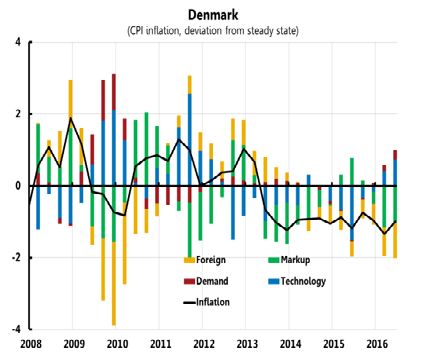
Figure 11
 RMSE of conditional forecast of HICP excluding energy and food
 (2012Q2 to 2014Q4)

 real + wages
 external
 benchmark: real domestic variables
 3

 2

 1

 0
 BE DE GR ES FR IT CY LV LT LU MT NL AT PT SI SK BG CZ HR PL RO SE UK

 Source: ESCB Staff estimations.
 Note: The RMSE is presented as a ratio to the RMSE associated with the real variables.

 2.2.2 Structural shock decomposition
Structural shock identification is Understanding the shocks that drive inflation is important to calibrate the appropriate
necessary to inform adequate
policy responses policy response. In principle, policy makers should pay more attention to domestic
 demand shocks than foreign supply ones, such as those related to oil price
 movements, unless these feed into agents’ expectations.

 The previous section discussed correlations between inflation and sets of variables,
 but did not offer any causal explanations. To be able to make causal inference, this
 section identifies structural shocks and quantifies their relative contributions to the
 dynamics of inflation since 2012. This section looks at headline HICP inflation. Since
 structural identification becomes more complicated as the number of variables
 increases, the Bayesian VAR used is smaller than the one in the previous section.
 The model contains seven variables, and seven shocks are identified and labelled
 using a combination of zero and sign restrictions. 13

 The seven shocks are labelled: “oil supply”, “global demand”, “domestic demand”,
 “domestic supply”, “short-term interest rate”, “spread” and “other”. The first two are
 global, while the other four are domestic. The seventh shock is not clearly
 interpretable and plays very little role in the dynamics of any of the variables except
 the exchange rate. For this reason, it could be interpreted as a genuine exchange
 rate shock, i.e. a movement in the exchange rate that does not depend on monetary
 policy or domestic supply shocks, etc.

 13
 For details, see Bobeica and Jarocinski (2017). For this exercise, a spread between long and short-
 term interest rates has been added to the previous set of variables to identify a nonconventional
 monetary shock à la Baumeister and Benati (2013).

 Occasional Paper Series No 181 / January 2017 – Empirical search for cyclical and trend
 determinants of low inflation: the validity of the Phillips curve and the risks of de-anchoring 20

The identification strategy builds on the different effects domestic and foreign shocks
 have on the relative growth rate of the euro area relative to the rest of the world to
 disentangle domestic from foreign demand and supply shocks. It also uses an
 identification scheme proposed by Baumeister and Benati (2013) for disentangling
 the effects of unconventional monetary policy in the United States, which singles out
 the transmission channel related to the compression of the spread between long-
 term interest rates and the policy rate. For the euro area the spread shock has a less
 clear-cut mapping to monetary policy, as the spread also responded strongly to
 market reactions to events unfolding during the sovereign debt crisis. This should be
 kept in mind when looking at the contributions from the spread shock. In this
 framework, the exchange rate is an endogenous variable and its response to, for
 example, monetary policy acts as a channel of transmission. This is discussed in
 detail in Section 4.3.2.

 As with the results from the previous exercise, domestic shocks became more and
 more important in the disinflation of 2012-2014. 14

 Figure 12 and Figure 13 show the historical decomposition of inflation (year-on-year
 change in headline HICP). The decomposition starts in 2012Q1; the blue line is the
 difference between the median unconditional forecast generated by the VAR and the
 actual series, and the bars show the effect of each shock.

Figure 12 Figure 13
Historical decomposition of headline HICP Historical decomposition of headline HICP – bundled
 domestic and global shocks
(yoy changes in HICP, deviation from baseline, percentage points ) (yoy changes in HICP, deviation from baseline, percentage points)

 headline inflation (deviation from mean) headline inflation (deviation from mean)
 oil supply global
 global demand domestic
 domestic demand other
 domestic supply
 spread
 interest rate
 other
 2 2

 1 1

 0 0

-1 -1

-2 -2

-3 -3
 Q1 Q2 Q3 Q4 Q1 Q2 Q3 Q4 Q1 Q2 Q3 Q4 Q1 Q2 Q3 Q4 Q1 Q2 Q1 Q2 Q3 Q4 Q1 Q2 Q3 Q4 Q1 Q2 Q3 Q4 Q1 Q2 Q3 Q4 Q1 Q2
 2012 2013 2014 2015 2016 2012 2013 2014 2015 2016

Source: Bobeica and Jarocinski (2017). Source: Bobeica and Jarocinski (2017).

 14
 For a similar result, see also Conti et al. (2017).

 Occasional Paper Series No 181 / January 2017 – Empirical search for cyclical and trend
 determinants of low inflation: the validity of the Phillips curve and the risks of de-anchoring 21

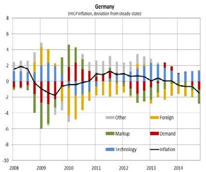
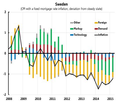
The structural identification also Although not shown in the figure, in early 2009 global demand shocks accounted for
identifies foreign (demand) drivers
in the first episode, but a larger role about 60% of the deviation of inflation from its unconditional path, while domestic
for domestic demand and supply in demand and spread shocks account for roughly 40% of it. The remaining shocks
the second
 mattered little in that episode.

 Since the end of 2012, the picture has been different: first supply shocks and then
 demand shocks started to turn negative. The contribution of the spread shock
 switched from restrictive to accommodative in 2014.

 These results are not far from those obtained using a DSGE model for the euro area
 (the New Area-Wide Model or NAWM), which finds that since the peak at end-2011
 the decline in inflation can be explained by the change in the contribution of mark-up
 shocks (2.1pp), especially in the goods market, and factors unexplained by the
 model (0.6pp). Across countries, mark-up shocks (both domestic and foreign)
 dominated in Spain, while in Germany foreign shocks were also important. This
 analysis is described in detail in Box 9.

 Having ascertained that domestic conditions have had a large role in determining the
 low inflation since 2012, the next section takes a closer look at the Phillips curve for
 both prices and wages to see how this workhorse for interpreting inflation dynamics
 over the business cycle fares in terms of explanatory power.

 2.3 Domestic drivers of inflation: are hybrid New Keynesian
 Phillips Curves (NKPC) useful in understanding inflation
 dynamics ex post? Do we see evidence of a changed
 responsiveness in inflation to economic activity?
The hybrid NKPC: the relationship The relation between economic slack and inflation as described by the Phillips Curve
between inflation and economic
slack and the role of expectations is of fundamental interest to central bankers, because an increase in inflation as
 economic slack becomes tighter is a precondition for monetary authorities to control
 inflation by the transmission of monetary policy actions through the real economy.
 This implies a positively sloped Phillips curve in the inflation/output gap space or a
 negatively sloped one in the inflation/unemployment space. The benchmark
 specification for the euro area is the following:
 
 = + − + + − + − + 

 where is the annualised quarter-on-quarter growth rate of the seasonally adjusted
 HICP excluding energy and food, is a slack measure, are survey-based
 
 inflation expectations and is the annual growth rate of import prices in euro from
 outside the euro area. 15 Both in the price and in the wage Phillips curve, inflation
 depends positively on expected inflation: an expected increase in prices will push
 labour unions to set higher wages today, and the resulting cost changes will be
 reflected in prices.

 15
 This specification does not allow for changes in indirect taxation and regulated prices, which can
 strongly influence the results in countries such as Spain (see e.g. Álvarez and Urtasun (2013)).

 Occasional Paper Series No 181 / January 2017 – Empirical search for cyclical and trend
 determinants of low inflation: the validity of the Phillips curve and the risks of de-anchoring 22

Changes in expectations of future A revision in inflation expectations (in turn possibly linked to changed monetary
inflation shift the Phillips curve
 policy credibility) or a change in wage and inflation mark-ups shift the Phillips curve
 up or down in the inflation/output space, affecting the intercept in the curve. 16
 Supply-side shocks that move inflation will also shift the curve. Finally, the slope of
 the curve can change over time. However, such changes are hard to distinguish from
 mismeasurement of economic slack.

The flexibility of the economy The responsiveness of prices to slack is related to the degree to which wages and
determines how responsive inflation
is to slack other costs react to economic conditions, and to a number of other factors, such as
 the frequency with which firms adjust prices. Box 4 shows evidence based on micro
 data that the frequency of price changes in Italy and Spain has increased in recent
 years, pointing to a potential steepening of the Phillips curve.

 The connection between inflation and economic slack is hard to pin down empirically
 due, for example, to mismeasurement of slack and expectations, or to exogenous
 shocks such as changes in indirect taxes.

Economic slack is unobservable Economic activity, and especially its potential level, is unobservable and
and multidimensional
 multidimensional, and there are advantages in using large dynamic models to
 estimate it. For instance, Jarocinski and Lenza (2016) use a dynamic factor model
 that performs a trend/cycle decomposition of real activity variables and core inflation.
 The model uses a single factor to capture common cyclical fluctuations and
 estimates the output gap as the deviation of output from its trend.

Alternative models can provide very Different assumptions, such as different sets of real activity indicators and different
different results on the size of the
output gap… specifications of the trend components of the variables, lead to different estimates of
 the output gap.

…and have different inflation How do different estimates of the output gap fare in terms of their ability to forecast
forecasting ability
 inflation? It turns out that the variants proposed by Jarocinski and Lenza (2016)
 associated with a continuation of a positive growth trend (thus implying a wider
 output gap) are the ones that produced better inflation forecasts over the period
 2002-2015. The best variant from this perspective would imply that the output gap
 was as large as -6% in 2014 (see the measure called Model 4 – no secular
 stagnation in Figure 14). Assuming the opposite, namely a break in the output trend,
 which we could relate to a secular-stagnation hypothesis, leads to a much poorer
 forecast ability of recent inflation. The output gap estimated by the IMF and the
 European Commission are halfway between the extremes arising from these
 dynamic factor models (see Figure 15). A caveat to these estimates is that they are
 obtained on the assumption that inflation reacts constantly to the output gap, and this
 issue – not just discerning how large the output gap is, but also separating the
 (mis)measurement of it from possible time variation in the Phillips curve – is central
 to understanding inflation dynamics and the recent overprediction of inflation.

 16
 On the anchoring of inflation expectations in the period under review, see Section 2.4.2.

 Occasional Paper Series No 181 / January 2017 – Empirical search for cyclical and trend
 determinants of low inflation: the validity of the Phillips curve and the risks of de-anchoring 23