On the Effects of COVID-19 Safer-At-Home Policies on Social Distancing, Car Crashes and Pollution - IZA DP No. 13255 MAY 2020
←
→
Page content transcription
If your browser does not render page correctly, please read the page content below
DISCUSSION PAPER SERIES

IZA DP No. 13255

On the Effects of COVID-19 Safer-At-Home
Policies on Social Distancing, Car Crashes
and Pollution

Abel Brodeur
Nikolai Cook
Taylor Wright

MAY 2020
DISCUSSION PAPER SERIES

IZA DP No. 13255

On the Effects of COVID-19 Safer-At-Home
Policies on Social Distancing, Car Crashes
and Pollution

Abel Brodeur
University of Ottawa and IZA
Nikolai Cook
University of Ottawa
Taylor Wright
University of Ottawa

MAY 2020

Any opinions expressed in this paper are those of the author(s) and not those of IZA. Research published in this series may
include views on policy, but IZA takes no institutional policy positions. The IZA research network is committed to the IZA
Guiding Principles of Research Integrity.
The IZA Institute of Labor Economics is an independent economic research institute that conducts research in labor economics
and offers evidence-based policy advice on labor market issues. Supported by the Deutsche Post Foundation, IZA runs the
world’s largest network of economists, whose research aims to provide answers to the global labor market challenges of our
time. Our key objective is to build bridges between academic research, policymakers and society.
IZA Discussion Papers often represent preliminary work and are circulated to encourage discussion. Citation of such a paper
should account for its provisional character. A revised version may be available directly from the author.

                                                     ISSN: 2365-9793

                                           IZA – Institute of Labor Economics
Schaumburg-Lippe-Straße 5–9                      Phone: +49-228-3894-0
53113 Bonn, Germany                             Email: publications@iza.org                                    www.iza.org
IZA DP No. 13255                                                                                              MAY 2020

            ABSTRACT
            On the Effects of COVID-19 Safer-At-Home
            Policies on Social Distancing, Car Crashes
            and Pollution*
            In response to COVID-19, dramatic safer-at-home policies were implemented. The
            understanding of their impacts on social distancing, travel and pollution is in its infancy. We
            pair a differences-in-differences framework and synthetic control methods with rich cellular
            tracking and high frequency air pollution data. We find that state and U.S. county safer-at-
            home policies are successful in encouraging social distance; beginning the day of the policy
            trips outside the home are sharply decreased while time in residence rises sharply. With
            less vehicle traffic, we find: a 50% reduction in vehicular collisions; an approximately 25%
            reduction in Particulate Matter (PM2.5) concentrations; and a reduction of the incidence of
            county-days with an air quality index of code yellow or above by two-thirds. We calculate
            that the benefits from avoided car collisions could range from $7 billion to $24 billion while
            the benefits from reduced pollution could range from $650 million to $13.8 billion.

            JEL Classification:             P48, Q53, Q58
            Keywords:                       COVID-19, safer-at-home, lockdowns, pollution, traffic,
                                            car crashes

            Corresponding author:
            Abel Brodeur
            Social Sciences Building
            University of Ottawa
            120 University
            Ottawa, ON K1N 6N5
            Canada
            E-mail: abrodeur@uottawa.ca

            * We thank Mohammad Elfeitori and Ramanvir Grewal for their excellent research assistance.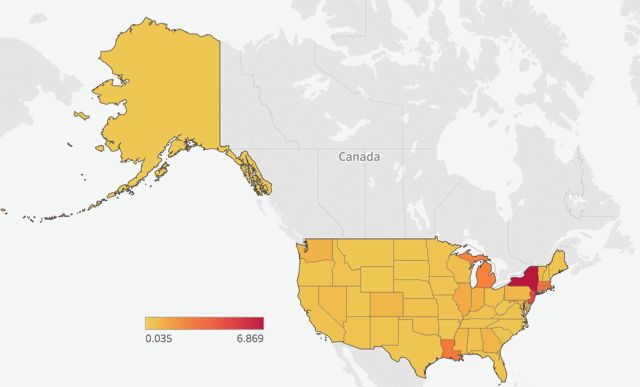
The emergence of COVID-19 (formally SARS-CoV-2 by the International Com-
mittee of Taxonomy of Viruses) has fundamentally changed human behavior. Char-
acterized as a pandemic by the World Health Organization on March 11, 2020, the
global scientific community is actively researching the virus and its impacts. This
pandemic has caused governments worldwide to implement curfews and safer-at-
home orders related to prevent further spread of the SARS-CoV-2.
    As of April 30, 2020 the U.S. has seen 29,000 deaths and over 1 million confirmed
cases. The first safer-at-home policy was implemented in California on March 19,
2020 and many states quickly followed suit; by April 30 all but 8 states had im-
plemented some from of lockdown order. To date, the focus of the debate over
safer-at-home orders has been on their efficacy and the tradeoff between lives saved
and reduced economic activity. An understudied aspect is the potential externalities
of safer-at-home orders on pollution and traffic.
    Identifying the causal impact of COVID-19 on pollution is difficult for a num-
ber of reasons. For instance, few recent reports and studies provide preliminary
(and suggestive) evidence that long-term exposure to fine particulate matter may
be associated with an increased risk of COVID-19 death (e.g., Wu et al. (2020)).
Moreover, the documented shortage of COVID-19 testing (and the willingness to
test) might be related to local pollution level. In this paper, we address these chal-
lenges by estimating the impacts of state and county safer-at-home orders instead of
the COVID-19 pandemic as a whole, and rely on a differences-in-differences frame-
work. This setting is attractive for at least two reasons. First, not all states (and
counties) have implemented safer-at-home orders and there is a great deal of varia-
tion in how fast they have been implemented. Second, our identification strategies
allow us to tackle issues of reverse causality and omitted variables bias by compar-
ing states (or counties) that implemented safer-at-home orders at different point in
time. Our identification assumption is that, conditional on the number of known
COVID-19 cases or deaths, the difference in pollution between states (or counties)
with and without safer-at-home orders would be constant over time. We relax this
assumption by also relying on synthetic control methods, matching counties based
on pre-policy pollution and population levels.
    We first investigate the impact of safer-at-home orders on pollution. We find that
state safer-at-home policies decreased air pollution (PM2.5) by almost 25%, with
larger effects for populous counties. This estimated effect is very large and suggest
that these policies reduce emissions by almost a half of a standard deviation. Our
estimates also suggest the issuance of a state order reduces the number of county-
days with an air quality index of code yellow or above by tow-thirds from 26%
to 9%. Similarly, we find that county safer-at-home policies have large impacts on
pollution, suggesting that local (county) government policies are equally as effective.

                                          2
We further explore the heterogeneous effects of safer-at-home policies on pol-
lution across county characteristics. We find that the decline in pollution from
safer-at-home orders is larger in more urban counties and smaller in counties that
voted for President Trump. Our results also indicate that counties with relatively
more young people and in states with a larger share of occupations than can be
done remotely experience a larger reduction in pollution form these policies.
We also investigate whether safer-at-home orders had an impact on social dis-
tancing using cell phone data from Google Inc. Community Mobility reports and
Unacast’s COVID-19 Toolkit. We first confirm the results of multiple working
papers that states’ implementation of safer-at-home policies significantly reduced
distance traveled.1 We also explore the heterogeneous impacts of safer-at-home
policies on different places visited using the Google cellphone data. We find that
safer-at-home policies significantly decrease the number and duration of trips made
to places of retail, grocery, parks, transit stations and places of work, and increase
time at home.
We further exploit the available data on social distancing to estimate how state
lockdowns, conditional on compliance (measured by the social distancing data)
reduce pollution. When controlling for visits to retail and recreation, grocery and
pharmacy trips, and commuting measures, our estimates decrease by approximately
16 percentage points, suggesting that social distancing partly explain the decline in
pollution.
In addition, we estimate the car collision externalities stemming from the safer-
at-home orders. We use data from five states where daily county data is available–
Alabama, Connecticut, Kentucky, Missouri, and Vermont and identify a large re-
duction - almost 50% - in traffic collisions after a state order is issued. We also
examine fatalities for the three states who report them–Connecticut, Kentucky, and
Missouri–with no evidence that fatalities are falling but mild suggestive evidence
that the risk of fatalities conditional on a crash is higher.
Lastly, we perform some back of the envelope calculations for the dollar value
benefit of our estimated reduction in pollution and car collisions from safer-at-home
orders. Using estimates of willingness to pay for pollution reduction based in the
U.S. we find the benefit from reduced pollution ranges from $650 million to $13.8
billion. Using estimates of the societal cost of car collisions from the National
Highway Traffic Safety Administration we find that the benefit from avoided car
collisions to range between $7 billion and $24 billion.
We contribute to a growing literature on the ongoing debate about safe-at-
home orders. We mostly relate to theoretical contributions relying on the SIR
1
See, for instance, Brodeur, Grigoryeva and Kattan (2020), who rely on Unacast data and
provide evidence that safer-at-home policies decreased total distance traveled.
3epidemiology model (e.g., Alvarez et al. (2020) and Jones et al. (2020)) or recent
policy proposals (e.g., Oswald and Powdthavee (2020)). Empirical contributions
have analyzed the determinants of safe-at-home orders implementation highlighting
a political partisan divide (Allcott et al. (2020); Baccini and Brodeur (2020)), its
consequences on mental health (e.g., Brodeur, Clark, Flèche and Powdthavee (2020);
Hamermesh (2020)), the economy (e.g., Atkeson (2020); Baker et al. (2020); Béland
et al. (2020)) and discrimination (e.g., Schild et al. (2020)). Last, a small literature
examines whether lockdowns are successful at preventing contagion (Friedson et al.
(2020)) and restricting mobility (Fang et al. (2020)). We believe our study is the first
large-scale empirical analysis of the environmental costs of safer-at-home policies in
the developed world. The most relevant paper is possibly He et al. (2020), which
provides evidence that lockdowns in China decreased PM2.5 by approximately 25%.
Last, our study contributes to a large literature documenting the impacts of
pollution and traffic on labor market outcomes.2 Ostro (1983) links air pollution in
the U.S. to lost work days and restricted activity days. Hausman et al. (1984) finds
that a one standard deviation increase in suspended particulates is associated with
an almost 10% increase in work days lost, after accounting for city fixed effects.
Graff Zivin and Neidell (2012) find that Californian farm worker output under
piece rate contracts is reduced by 5.6% for a one standard deviation increase in
air pollution.3 Ebenstein et al. (2016) studies show that performance on strictly
scheduled yet high stakes exams declines with exam day air pollution - and as a
result have lasting impacts on post-secondary educational attainment and earnings.
To the extent that air pollution reduces labor supply and its productivity, safer-at-
home orders may have a lasting legacy of increased - home based - labor.
Researchers have also identified health consequences of air pollution exposure
and extreme traffic; short-term exposure to air pollution impacts heart and lung
function (Seaton et al. 1995), irritates the throat and eyes (Pope 3rd 2000), causes
headaches (Szyszkowicz 2008) and induces elevated levels of stress hormones (Li
et al. 2017).4 It has also been connected to psychological symptoms such as in-
creased anxiety(Power et al. 2015), reduced pro-social attitude (Lu et al. 2018), de-
pressive sentiment (Szyszkowicz 2007) and increased suicide propensity (Yang et al.
2011). Our finding of decreased pollution thus provides a plausible mechanism for
2
Our study also adds to a growing literature on the consequences of COVID-19 (Alon et al.
(2020); Atkeson (2020); Berger et al. (2020); Binder (Forthcoming); Briscese et al. (2020); Fang
et al. (2020); Fetzer et al. (2020); Jones et al. (2020); Ramelli et al. (2020); Stephany et al. (2020);
Stock (2020)).
3
Adhvaryu et al. (2014) study the productivity of garment factory workers in Bangalore and
find that a one standard deviation increase in air pollution resulted in a loss of 6% worker efficiency.
Chang et al. (2019) study the productivity of white collar (call center) workers in China; higher
daily levels of air pollution impact number of calls serviced.
4
Traffic congestion has been linked to domestic violence (Beland and Brent (2018)), stress
(Stutzer and Frey 2008) and unhappiness (Anderson et al. 2016).
4the documented decrease in Google Searches for the topic ‘Suicide’ following the
implementation of safer-at-home policies in the U.S. and Europe (Brodeur, Clark,
Flèche and Powdthavee (2020)).
The rest of the paper is organized as follows. Section 1 details the data collection,
while section 2 describes our methodology. We discuss the impacts of safer-at-home
policies on pollution in section 3. In Section 4 we rely on cell phone data to document
changes in travel behavior. Section 5 investigates the effects of state and county
policies on collisions. Last, Section 7 concludes.
1 Data and Identification Strategy
In this section, we describe our data. We first provide information on COVID-19
cases and fatalities, and how they vary over time and across states. We then describe
the determinants of implementing stay-at-home orders and our social distancing
data. Last, we describe our pollution and collision data.
1.1 COVID-19 Known Cases and Deaths
The first case in the U.S. was a man who had returned from Wuhan, China to
Washington State. The case was confirmed on January 20, 2020. Six additional
states had confirmed cases later in January and February. The first case of commu-
nity transmission was confirmed in California, on February 26, 2020. As of April
30, 2020 there were over 1 million confirmed cases due to COVID-19 in the U.S.
The COVID-19 known cases and deaths data comes from the Github repository
associated with the Johns Hopkins University interactive dashboard. The data
are available here: https://github.com/CSSEGISandData/COVID-19. Appendix
Figures A1 and A2 illustrate the geographic distribution of COVID-19 knowns cases
and deaths per 10,000 inhabitants, respectively. The states of New York and New
Jersey had the highest death rate as of mid-April, 2020.
1.2 Safer-at-Home Policy
Figures 1 and 2 present maps of counties and states that implemented a safer-at-
home policy, prior to April 30, 2020, respectively. Nearly all states had implemented
such a policy at this point in time. But the timing of implementation varies consid-
erably. The first state to implement a safer-at-home policy was California on March
19th, 2020. 18 more states followed California in the following week. As of April 30,
2020, 43 states (including the District of Columbia) had implemented some form
of lockdown, representing 1,453 counties. 148 counties implemented a county-level
safer-at-home policy, of which 141 are located in states that would eventually have
5a statewide policy. The median county implemented its safer-at-home policy one
week prior to the statewide policy.5
1.3 Social Distancing Data
We extract data on social distancing from the from Google Inc. Community Mobility
reports and Unacast’s COVID-19 Toolkit. Our main data source is Google, and rely
on Unacast’s data as a robustness exercise.6 Table 1 provides summary statistics
for our Google and Unacast indexes.
Google Inc. released data on social distancing practices at the daily level for
United States Counties.7 The datasets are presented as percent changes in how visits
and length of stay to places (like grocery stores or parks) compared to a baseline
for the same areas and the same day of the week. The baseline is computed using
data from January 3, 2020 to Feb 6, 2020. While the accuracy of cellular tracking
data will vary from region to region, our identification is necessarily within region.8
People’s activities are coded into one of six categories: grocery and pharmacy,
parks, transit stations, retail and recreation, residential, and workplaces.9 The
data, derived from the Location History of someone’s Google Account represents a
sample of users - of course this may not reflect the broader population.
We also rely on daily data from Unacast’s COVID-19 Toolkit. Unacast provides
a Social Distancing Scoreboard at the county-level using cell phone data which aims
to empower organizations to evaluate the effectiveness of social distancing initiatives
(Brodeur, Grigoryeva and Kattan (2020)). Using data pre-COVID-19 outbreak as
a baseline, Unacast computes rate of changes in average distance travelled, non-
essential visitation, and human encounters. For our analysis, we rely on the first
two indexes. Non-essential visits include many places such as cinemas and cloth-
ing stores. More details are provided here: https://www.unacast.com/covid19/
social-distancing-scoreboard. Non-essential locations were determined by Un-
acast, following guidelines issued by various states.
5
Only seven counties (Brazos, Comal, Humboldt, Kings, Mendocino, Merced and Milam)
implemented a safer-at-home policy after a statewide policy.
6
Unacast’s data does not allow us to investigate social distance practices by categories, e.g.,
grocery stores or workplaces. Moreover, the data is unavailable for many counties.
7
This temporarily available dataset is intended to help remediate the impact of COVID-19. It
is available here: https://www.google.com/covid19/mobility/.
8
The data is coded as missing if there are insufficient levels of data to be statistically significant.
9
Grocery and pharmacy: grocery markets, food warehouses, farmers markets, specialty food
shops, drug stores, and pharmacies. Parks: local parks, national parks, public beaches, marinas,
dog parks, plazas, and public gardens. Transit stations: public transport hubs such as subway,
bus, and train stations. Retail and recreation: restaurants, cafes, shopping centers, theme parks,
museums, libraries, and movie theaters. Residential: places of residence. Workplaces: places of
work.
61.4 Pollution Data
Air pollution data is from in situ monitors and provided by AirNow, a partnership
between United States agencies.10 The primary pollutant we use in our analysis
is particulate matter with diameters less than 2.5 micrometers - capable of being
inhaled and passing the blood brain barrier. Emissions from combustion of gasoline,
oil, diesel fuel or wood produce much of the PM2.5 pollution found in outdoor
air. PM2.5 is also associated with the greatest proportion of adverse health effects
related to air pollution in the United States.
The Environmental Protection Agency monitors PM2.5 levels to protect public
health and the environment, and has found average decreasing trends in the last
two decades.
To aggregate PM2.5 levels from the monitor level to the county level, we assign
each county’s population weighted centroid to the nearest air quality monitoring
station, but only if that station is within 50 kilometers as accurate PM2.5 levels are
necessarily local. The minimum distance to a pollution monitoring station is 114
meters, while the mean and median are approximately 25km away.
In Figure 3 we present average weekly PM2.5 levels by county for the week
of March 1-7, 2020. This period, prior to any lockdown orders serves as a visual
representation of the geographic distribution of air pollution levels. In Figure 4 we
present the same PM2.5 measures during the final week of April - after all eventually
treated states had implemented a stay at home order.
While a derivative of PM2.5 levels, we also provide results using Air Quality
Index data. This unit-less measure ranges from 0 to 500, with a score below 50
representing no harmful levels of air pollution.
1.5 Collision Data
For our analysis on car crashes, we rely on collision data at the county-level from
five states: Alabama, Connecticut, Kentucky, Missouri and Vermont. The data
were scraped from the data portal Safe Home Alabama, Connecticut Car Crash
Data Repository, Kentucky State Police, Missouri State Highway Patrol and the
Vermont Public Crash Data Query Tool. The remaining states are excluded for
four reasons: (1) data portal unavailable during the pandemic making it impossible
to scrap the data; (2) request for data under review (with longer delays due to the
pandemic); (3) data unavailable at the county-level; and (4) data available only at
the month or year-level.
10
U.S. Environmental Protection Agency, National Oceanic and Atmospheric Administration
(NOAA), National Park Service, NASA, Centers for Disease Control, and tribal, state, and lo-
cal air quality agencies. The centralized system provides uniform quality control and reporting
consistency.
7Our main variable of interest is the daily number of collisions per county. We
also rely on the number of car crash fatalities for one state (Kentucky).
2 Identification Strategy
2.1 Differences-in-Differences
Our hypothesis is that safer-at-home policies decreased PM2.5 concentrations, es-
pecially through a decrease of pollution generating behaviors. To investigate this
hypothesis, we estimate the following specification:
0
ycst = α + βStateSaf erst + λCountySaf ercst + γc + δt + Xcst ω + εcst (1)
where ycst is daily average Particulate Matter 2.5 in µg/m3 in county c in state s
and year t. We include a full set of county dummies γc to control for time-invariant
county characteristics and date (e.g., a separate dummy for March 1, 2020, March
2nd, 2020, etc.) dummies δt . The time period is January 1st, 2020 through April
30th, 2020. The state-level variable StateSaf erst equals one once the state has
issued the order and zero for the pre-policy period. Our primary coefficient of
interest is β. (We also investigate the impact of county orders. The county-level
variable CountySaf erct equals one once the county has issued the order and zero for
the pre-policy period. The coefficients of interest here is thus λ. For this analysis,
the sample is restricted to counties that eventually implement a county order.)
Note that the adoption of safer-at-home policies and timing of adoption msy be
endogenously related to the severity of the virus. We thus include, Xcst , a vector
of county-day level covariates including COVID-19 known cases and deaths per
10,000 people. The county population data comes from 2019 Census estimates. We
cluster standard errors at the state-level, corresponding to the primary policy and
treatment level.
Our identification assumption is that, conditional on controls, the evolution of
PM2.5 for counties with safer-at-home policies would not have been different from
those without the policies. This amounts to an assumption of parallel trends in
PM2.5 for treated and untreated counties.
2.2 Synthetic Control Methods
We complement our difference-in-difference estimates with those from a synthetic
control methods approach. The main concern with the estimates from the difference-
in-difference approach comes from the lack of an appropriate comparison group in
the post period. These comparison groups, depending on the date, are either a)
8counties that have not yet had a state order applied to them b) counties that will
never have a state order applied to them, or c) simply the pre-period of the treated
counties. To tease out inference from issues of selection (as in a) and b) or issues
of trends (as in c) we turn to the synthetic control method. The synthetic control
method addresses this problem by constructing a counterfactual evolution of PM2.5
from a weighted convex combination of others.
This method requires ‘donor’ counties - counties that are not or are not yet
treated - to donate their PM2.5 evolutions to those that are treated. In our appli-
cation, we restrict donor counties to have populations within 2000 of their treatment
county so that we are comparing equally populous areas with each other. We also
require counties to have similar pre-COVID PM2.5 average concentrations, within
2 µg/m3 .
To construct our synthetic matching, we follow the steps in Abadie et al. (2010).
The idea of this method is to match a treated county (with a state order) to a group
of control counties having similar pollution - and population levels - prior to the
order’s implementation. The hypothesis is that the treated and control counties
would have a similar change in pollution if the order had not been implemented.
We construct a synthetic match for each of the treated counties by solving the
following optimization problem and finding the optimal vector of weights:
" #2
∀i ∈ N,
XX X
wji∗ j∈U wji wji Yjt
= arg min Yit −
i t j
Subject to
wji = 1 and ∀j ∈ U, ∀i ∈ N, wji ≥ 0,
X
j
Where Yit is the pollution for county i ∈ N on pre-event t ∈ T. N being the
set of treated counties and T the set of pre-order dates. wji is the weight given to
county j ∈ U, the set of control counties.
The pollution level for each synthetic county is constructed as:
X
Ybit = wji∗ Yjt
j
.
The estimates are put together in the same manner as regressions elsewhere in
the paper. Each county is equally weighted. (In Appendix Table A2 we demonstrate
the robustness of the synthetic control estimates to the inclusion of weights, since
donor states were necessarily similar in population to treatment states.)
93 Stay-Home Orders and Pollution
In this section, we present the main results beginning with our differences-in-
differences strategy. We then then provide additional results obtained using syn-
thetic control methods.
3.1 Differences-in-Differences
In Table 2 we present our main result: a state’s implementation of a stay-at-home
order significantly lowers pollution for its counties.
This table presents estimates of Equation 1 in which we compare counties in
states with and without a statewide stay-at-home order. In all columns the depen-
dent variable is PM2.5 concentration. As noted in Section 1, the sample is restricted
to counties with a reasonable degree of accuracy in the dependent variable - counties
with a population weighted centroid within 50 km of an air pollution monitoring
station. We use a total of 1,472 counties in our estimation.
In the first column, we include only date and county fixed effects. The estimate
for our statewide stay-at-home order is statistically significant at the 1% level and
suggests that the introduction of a state order reduces PM2.5 levels by 1.6 µg/m3 .
With a mean of the dependent variable almost 7 (the regression constant in this
specification is also the average PM2.5 concentration in the pre-policy period), this
suggests the policy decreased air pollution by almost 25%. For additional context,
the standard deviation of PM2.5 before any state orders were implemented is 3.4
µg/m3 , suggesting the policy reduces emissions by almost one half of a standard
deviation.
In the second column, we include the number of confirmed COVID-19 cases per
10,000 people as a control. In the third column, we replace the number of confirmed
cases by deaths attributable to COVID-19, again per 10,000 people. The estimates
are negative, suggesting that increased cases or increased deaths reduces PM2.5 in
a county, although neither are statistically significant at conventional levels.
In the fourth column, we re-estimate the unweighted estimate from column 1
now weighted by county population. In this manner, we are now putting more
weight on relatively more populous (and polluted) counties. The inclusion of this
weighting increases the effect estimate by more than 50% from 1.6 to 2.5 µg/m3 ,
suggesting that the decrease in PM2.5 was larger for more populous counties.
In columns 5 and 6, we re-estimate population weighted averages of columns 2
and 3. We find that increased confirmed cases, and in particular higher COVID-
19 death rates significantly reduce the air pollution - conditional on a state order
being in place. This does not come as a surprise as human behavior and compliance
with state orders may be a function of COVID-19 rates. We examine possible
10mechanisms later.
In Table 3 we conduct a similar but distinct analysis. While in Table 2 the
dependent variable was PM2.5 concentration, in Table 3 we change the dependent
variable to an indicator that takes a value of one if the PM2.5 level in that county,
and on that day, is below the National Ambient Air Quality Standard of 12 µg/m3 .
This analysis is important as Bowe et al. (2019) show that, among a cohort of U.S.
veterans, nine causes of death were associated with PM2.5 exposure below standards
set by the Environmental Protection Agency.
The specifications and structure of the table remain the same as in Table 2.
Instead of measuring the reduction of PM2.5 levels, we now measure increases in
safety. The interpretations of the coefficients change as well. For example, in column
1, nearly 90% of days prior to a state order have an acceptable level of ambient
air pollution. When state orders are introduced almost all days, for all counties,
have acceptably clean air. In column 4, when population weights are introduced,
only 74% of county-days have an acceptable PM2.5 level (corresponding to more
populated areas having higher levels of ambient air pollution). When the state order
is implemented, the proportion of acceptable air days increases by 16 percentage
points (a 22% increase).11
In Table 4, we examine how county level orders, which are typically implemented
before associated state orders, affect ambient pollution levels. The sample is nec-
essarily restricted to counties that at some point implement a county order. In the
first column, the effect of the state issuing an order is a reduction of 2.8 µg/m3 ,
larger than previous estimate of 1.6 µg/m3 (note however, the percentage reduction
is essentially the same). While the set of counties that issue their own order have
higher pollution levels on average, when their state issues an order their air pollution
reduction is proportional to other counties. The second estimate is the additional
reduction attributable to the county order. The estimate is negative, suggesting
further reduction in PM2.5, however it is not statistically significant. Controlling
for COVID-19 cases or deaths, as in columns 2 and 3 does not meaningfully disturb
this finding.
In columns 4-6, we leverage the time between a county and state issue their
respective orders (median of 7 days). By restricting the estimation sample to the
time period before the state issues the order, we can estimate the effectiveness of
the policies available to counties. During this short time frame, the effect of a
county order is roughly the same as a state order. Combined with the results from
the previous columns, this suggests that counties have the ability to significantly
reduce PM2.5 emissions by unilaterally issuing safer-at-home orders, however their
11
In Appendix Tables A4 and Table A5 we use instead Air Quality Index and an indicator for
an acceptable Air Quality Index of below 50, respectively. Estimates are substantively the same.
11effectiveness is subsumed by the overarching state authority.
In Appendix Table A1, we further demonstrate the robustness of the effects
of state orders on ambient PM2.5 levels to county level government safer-at-home
orders. In column 1 we re-produce our main result for all counties. There is a subset
of counties that issue their own orders prior to their respective state. In column
2, the constant coefficient indicates this set of counties had higher PM2.5 levels on
average. The reduction in PM2.5 levels from a state order is proportionally larger
- such that a state order reduces pollution by 25% in counties that did and did not
issue their own orders. The estimate of the effect of a county order is negative,
but not statistically significant, suggesting that conditional on a state order being
present, there is minimal additional reduction in PM2.5 from an additional county
order being in effect. In column 3, we confirm that state orders were also effective in
the majority (1362) counties that did not issue their own order - important as the set
of counties that issue their own orders could be driving the results for all counties.
The estimated effect of a state order is statistically significant and reassuringly close
to the average estimate from column 1. Columns 4 through 6 repeat these exercises
controlling for the COVID-19 cases in each county - likely correlated with when a
county or a state is would issue a state order. The estimated effect size of state
orders is reassuringly undisturbed.
3.2 Graphical Evidence
We provide a visual summary of the pollution impact in Figure 5. This figure
plots estimated PM2.5 levels at daily intervals pre- and post-statewide order. The
Equation is:
40
X
ycst = α + βn (DaysSinceLockdown = n) + γc + δt + εcst (2)
n=−60
This specification decomposes the level of PM2.5 by the number of days since
(and before) the state order. The regression includes county and date fixed effects,
controlling for national level changes in PM2.5 as, for example, the country comes
out of winter. We plot the estimated difference between PM2.5 levels compared to
the date that the state order was implemented (which is set to zero). The time
window is 60 days before to around 45 days after the policy is implemented. The
dashed lines represent robust 95% confidence intervals.
Figure 5 shows that PM2.5 levels, within-county, were stable if not increasing
from 60 to 15 days prior to the statewide order. Around two weeks before state
orders came into effect (on average March 28) we begin to see a reduction in PM2.5
emissions, with an even larger decrease in the days following the implementation.
12The negative impact is at its largest at the end of the time window, i.e., 45 days
after the safer-at-home implementation, suggesting that adding more days to our
sample post-state policy would serve to only increase our point estimates.
Why does pollution register a decrease in the days before the policy? One
explanation is that the announcement of the safer-at-home policy typically precedes
the implementation by 3–4 days. Another explanation is that a partial lockdown,
which includes school and venue closures, may have already been implemented in
these counties days before the full safer-at-home date was implemented. It may also
reflect people’s anticipation of the impending policy date based on their observation
of the pandemic or neighboring states that had entered safer-at-home policy earlier.
We explore this last possibility in Section 4.
3.3 Synthetic Control Methods
The Differences-in-Differences estimates presented above indicate a large reduction
in PM2.5 after a state issues stay-at-home orders. We now turn to our synthetic
control methods analysis as a robustness check.
In Appendix Table A2 we present the results of applying synthetic control meth-
ods to create, county-by-county, counterfactual levels of PM2.5. This method re-
quires ‘donor’ counties (counties that will never, or at least do not yet have a
state order in place) to donate their PM2.5 time series evolutions to those that are
treated. In our application, we restrict donor counties to have populations within
2,000 of their treatment county so that we are comparing equally populous areas
with each other. We also require counties to have similar pre-COVID PM2.5 average
concentrations, within 2 µg/m3 .12
When combined with the observed reduction in PM2.5, the difference between
observed (the treated) and the counterfactual (the synthetic control) is very large
and statistically significant. In the first column, the dependent variable is this
difference; compared to their counterfactual, treated counties reduce their PM2.5
levels by more than 2.5 µg/m3 on average. The addition of COVID-19 known
cases or deaths does not substantially disturb the results. Including populations
weights no longer increases the effect sizes of the estimates, unsurprising as we now
restrict the counterfactual to combinations of counties with approximately the same
population.
In Appendix Figure A3 we present these results graphically. We see that the
levels of pollution are relatively similar for the two sets of counties prior to the state
order. Once the state order is implemented, there is a large decrease in pollution in
treated counties, which persist over the entire month following the implementation.
12
Our results are robust to other cut-offs. Estimates available upon request.
13Appendix Figures A4 and A5 plot the evolution of PM2.5 in the treated and
synthetic control counties, respectively. This split allows us to see whether the
decrease in pollution occurs because of treated counties reducing their emission
or counterfactual counties increasing their emission. The time period is 30 days
prior to 30 days after state orders. We find no changes for counterfactual counties,
while the changes for treated counties are strikingly similar to the ones presented
in Appendix Figure A3.
3.4 Heterogeneity: Urbanization, Republicans and Work from Home
We investigate whether the magnitude of the documented effect of safer-at-home
policies on pollution is related to county-level characteristics in Appendix Table
A7. More precisely, we test whether more urban, younger and democrat counties
experienced a larger decrease in PM2.5 following the implementation of a safer-
at-home order.13 In columns 1–2, we split the sample for over and below county
urbanization of 50%, respectively. We find that the estimated decrease is about
33% larger for urban counties than rural counties, confirming our previous finding
that more populous counties are more affected by state orders.
In columns 3–4, we restrict the sample for counties in which a majority of vot-
ers voted for President Trump during the last Presidential Election. Column 4
restricts the sample to the other counties. We find that the decrease in pollution is
much smaller in counties that supported President Trump. This finding is in line
with Engle et al. (2020), who document that counties with lower share of votes for
republicans comply more with stay-at-home orders.
Columns 5 (6) test the effect of safer-at-home policies for counties with relatively
more (less) individuals aged at least 65 years old (split by median). We find that
counties with relatively more young people experience a larger decrease in PM2.5,
perhaps due to more work being done remotely post-lockdown.
We explore this possibility in columns 7–8. We split the sample into counties
within states with above and below median values of the share of occupations that
can be done from home. These classifications of the feasibility of working form in a
given occupation come from Dingel and Neiman (2020) and code provided by those
authors and Ole Agersnap. Column 7 (8) corresponds to counties in states with an
above (below) median share of occupations able to be done from home. We find
that counties in states with a greater ability to work from home experience a larger
decrease in PM2.5.
13
Data on the share of urban population is based 2010 Census data. Urbanization rate comes
from the American Community Survey (ACS-5 years estimates).
144 Stay-Home Orders and Social Distancing
We now investigate the impacts of safer-at-home policies on trips pattern. We
first rely on the Google Inc.’s COVID Community Mobility Report, leveraging the
Location History of Android phone users.14
In Figure 6, we plot estimates of Equation 2 for the change in retail and recre-
ation time provided by the social distancing data. We see a rising pattern until
about 14 days before a state policy is issued. Once the state is 14 days from an-
nouncing a state order, the level of trips taken for this non-essential behavior begins
reducing, likely reflecting the underlying conditions that ultimately predict a state
order being issued. Notably, the day after a state issues an order sees a large and
discontinuous jump in the level of retail and recreation visits.
In Figure 7, we present the change in grocery store and pharmacy time. As a
behavior its notable that this is often considered essential. This behavior seems to
be much less sensitive to underlying conditions - there is very little curvature like
that for retail and recreation - but responds swiftly and discontinuously to the state
order. (Of anecdotal note is that the day before the state order was issued but after
it was announced, there is a sharp increase in the visits to grocery stores).
In Figure 8, visitation of local and national parks, there is a generally increasing
trend leading up to (and after) the state order.The week following a state order sees
a negative dip in visitation, however the estimates quickly become positive. This is
unsurprising as it is unclear whether visitation to parks should decrease given social
distancing orders - this may be left to the state order policy.
In Figure 9, we plot the evolution of trips to transit hubs. These include railway
stations as well as subway when available. Some of these visits are undoubtedly
long distance trips that are canceled both leading up to and directly after the state
issues an order, as well as commuting patterns. This is further examined in Figure 10
which measures trips and length in workplace areas. Around the two weeks leading
up to the state order, workplaces trips begin to decrease. The day of the state
order sees a large - and discontinuous - fall in time at work. Workplace attendance
mirrors PM2.5 levels, decreasing after the order is given.
The final social distance measure is whether people are staying at home - the
prescribed place to be under the sort of orders the states issue. We see an evolution
that is close to the inverse of what we see for workplace time - about two weeks
leading up to a state order to be home, there is some increase in time spent in
residence. Compared to the day of implementation, the next day sees a large and
discontinuous increase in time spent at home. The trend continues - mirroring in
14
While estimates vary, Android comprises between 40–60% of the US market share, of approx-
imately 270 million devices.
15the literal sense - the trends seen for other social distance measures.
We confirm these findings in Table 5. The dependent variable in the first column
is the percentage change in the number and duration of trips made, by county
to places of retail and recreation. The dependent variable in the second column
is grocery store and pharmacy trips. Trips to parks, which includes local parks,
national parks, public beaches, marinas, dog parks, plazas, and public gardens is
the dependent variable in the third column. The fourth column is public transit
stations - subway bus and train stations. The fifth and sixth columns’ dependent
variables are visits to places of work (not necessarily working) and places of residence
(established during the baseline period in January). Regardless of the measure of
social distancing behavior, the implementation of a state order significantly reduces
social contact. In other words, safer-at-home policies increase time in residential
areas, which increases social distance, but not necessarily familial distance.
These results provide suggestive evidence that safer-at-home policies partly de-
crease pollution by decreasing the number and duration of trips. In Table 6 we
confirm the effects of each of Google Inc.’s COVID social behaviors on ambient
PM2.5 levels. Leveraging the entire data period (beginning February 15, 2020) we
see that behaviors that take people out of the house (retail and grocery shopping,
visiting national parks, commuting to work) all increase ambient pollution levels
while more time spent at home reduces PM2.5 concentrations.
In Table 7 we examine how state lockdowns, conditional on reducing these be-
haviors, reduce pollution levels. Because we do not have data for all counties and
all dates (for privacy reasons), the set of counties studied is necessarily a subset of
those examined in Table 4. For this reason, in the first column we present the basic
specification once again but for our restricted (balanced) sample. For the counties
with social distancing data, the introduction of a state order reduces PM2.5 levels
by around 1 µg/m3 . Controlling for visits to retail and recreation, grocery and phar-
macy trips, and commuting all reduce (slightly) the estimated effect of the policy,
individually and collectively in the final column. The inclusion of these variables
decreases the size of our statewide policy by about 16 percentage points.15
4.1 Unacast’s Social Distancing Indicators
We now test the robustness of our results by using other metrics of distance traveled.
More specifically, we examine how state orders affect total distance traveled (ADT)
and non-essential visits using Unacast cell phone data.
A number of validation layers occurred to create the metrics. First, ADT cor-
relates well with the number of confirmed COVID-19 cases: the more cases are
15
We include in our estimation the variables that state lockdowns had an unambiguous effect
on, see Figures 6 through 11.
16confirmed, the greater the decrease in the average distance traveled an the county-
level. For cell phone data in particular, it works independently of information flow
disruptions - the metric is unaffected due to cellular inactivity if people are dwelling
at home. The metric (while admittedly simple) captures how people adapt their
everyday behavior. Working from home, reduction or elimination of trips to enter-
tainment or spare-time facilities, and canceling vacations all reduce travel distance.
Our estimates using Unacast data are presented in Appendix Table A3. The
dependent variable is our two indices of total travel distance in columns 1–3 and
non-essential visits in columns 4–6, respectively. In the first column, we see that, on
average distance travelled fell by 3.3 percentage points under a state order. Columns
2 and 3 add to the model COVID knows case and death rates, respectively. We
find that COVID-19 known cases per capita also reduce travel. Unsurprisingly,
increased death rates also reduce observed cellular movement patterns. Since it is
very plausible that a person could travel 50 feet in one area and meet many people
- and in another not meet a soul, we examine the number of non-essential places
visited in columns 4–6. Results are quantitatively similar - state orders reduce the
likelihood to visit non-essential places by 6 percentage points.
5 Stay-Home Orders and Collision
Social distancing can result in fewer cars on the road, reducing emissions of air
pollution and also reducing the number of collisions or fatalities experienced. Motor
vehicle collisions are one of the leading causes of deaths for Americans - beaten
only by heart disease, malignant neoplasms and unintentional poisoning. (Both
heart disease and malignant neoplasms have been connected to PM2.5 exposure.)
In this way, state orders may save even more lives than intended. We collected
traffic collisions data at the county-day level for Alabama, Connecticut, Kentucky,
Missouri, and Vermont. There are an average of 6.2 car crashes from January 22nd,
2020 through April 30th, 2020.
In Table 8, we estimate the effects of state orders on the collision incidence rate
in a county, per day. We present the incidence report ratios of a Poisson count model
with county and date fixed effects. In the first column, we estimate that a state order
reduces the incidence of collisions by almost two thirds. Taking the approximately
6 crashes per day, this results in a reduction of 4 collisions per day, per county. In
columns 2–3, we introduce the number of COVID-19 cases and deaths, respectively.
Regardless of the underlying severity of the infection, the effectiveness of the state
order remains large and statistically significant. In the fourth column, we introduce
three measures of social distancing: grocery and pharmacy, retail and recreation,
and workplaces. Introducing these measures in the model helps accounting for the
17direct channels through which the state orders should be operating. We find that
the effect estimate for a state order down to 45% (from about 60%).
Overall, these results suggest that safer-at-home policies had very large impacts
on traffic collision, in part due to a decrease in visits to places such as groceries and
workplaces.
Last, we rely on fatalities for one state, Kentucky. The estimates are presented
in Appendix Table A8. In all columns, the estimated effect of a state order is
statistically significant - the introduction of a state order drastically reduces fatal
collisions. In the second column, we control for the count of collisions. As ex-
pected, more collisions lead to an increase in fatal collisions. The estimated effect
of fatal collisions falls to around a one-half reduction. Increased COVID-19 deaths
correspond to greater fatality rates as well.
6 Interpretation
In this section, we provide back of the envelope calculations of the pollution and
collision externalities generated by safer-at-home orders.
Our calculations here are, in part, based on the growing literature estimating
the revealed - rather than stated - willingness to pay (WTP) for air quality. Currie
et al. (2015) exploit the effect of toxic plant openings to estimate the impact of air
quality on house values and lifetime earnings due to depressed birth weights. Recent
work by Ito and Zhang (2020) using purchases of air purifiers in China suggests that
the WTP for 1 µg/m3 reduction of PM10 is $1.34 annually. Chay and Greenstone
(2005) find that the elasticity of housing values to particulates ranges from -0.2 to
-0.35. Deschênes et al. (2017) estimate the WTP for nitrogen oxides reductions.
Barwick et al. (2017) estimate a lower bound of the annual WTP for a 10 µg/m3
reduction in PM2.5 in China is $9.25 per household. Finally, Bayer et al. (2016)
estimate the WTP to avoid ozone using house purchases in the San Francisco Bay
Area, finding a 10% reduction in pollution commanded a price of up to $300.
Our estimates from Table 2 indicate that the introduction of safer-at-home or-
ders decreased pollution by 1.6–2.5 µg/m3 . Despite the estimates being for PM10,
if we were to apply the WTP estimates of $ 1.34 per 10 µg/m3 annually reduction
from Ito and Zhang (2020) to our findings and prorate it for the average number
of lockdown days (85,119 county-days / 1453 counties = 58.6 days), we obtain es-
timates of $0.034–$0.054 per household. As there are 114,951,213 households in
the U.S. that are affected by safer-at-home orders (Census Estimates, American
Community Survey 2018), that translates to an estimated benefit ranging from $3.9
million to $6 million. If instead we use the PM2.5 specific estimates of WTP from
Barwick et al. (2017), the estimated benefit falls between $27.3 million to $42.6
18million.
Borrowing from Bayer et al. (2016) who find American home owners are willing
to pay between $60-$300 annually for a 10% reduction in one pollutant, the WTP
associated with our estimated 25% reduction in PM2.5 could be as high as $150-
$750 annually per household.16 Furthermore, Bayer et al. (2009) estimate that the
marginal WTP for a 1 µg/m3 reduction in PM10 for 1 year to be $22 per household.
Using these estimates of WTP from the more appropriate American samples
we instead find estimated benefits of $650 million to $1 billion using the adapted
WTPs from Bayer et al. (2009), and $2.7 billion to $13.8 billion using the adapted
estimates from Bayer et al. (2016). These estimations vary widely, no doubt due
to the many assumptions necessary to compute figures at such an aggregate level.
However they serve to give a sense of the scale of the possible environmental benefits
these orders have.
There are extensive costs associated with traffic collisions, from congestion im-
pacts; to medical and repair bills; to loss of life. We can generate rough estimates
of the benefits of reduced collisions using 2013 estimates provided by the analytics
company ISO that the average collision claim was $3,144 USD (about $3,500 USD
in 2020): http://www.rmiia.org/auto/traffic_safety/Cost_of_crashes.asp.
Alternatively, the National Highway Traffic Safety Administration (NHTSA) esti-
mated that the economic cost of the 13.6 million motor vehicle crashes was $242
billion , for an average cost of $17,794 (2010 dollars, $ 21,054 in 2020) per crash.17
When accounting for quality-of-life valuations, the estimates are $836 billion in
costs, for an average of $61,470 (2010 dollars, $72,732 in 2020) per crash.
If taken to the national-level and not restricting to our PM2.5 data, 2,628 distinct
counties were subject to a state order by April 30th, 2020. Their combined total of
lockdown-days was an estimated 85,119. If the reduction in the fi
ve states in our sample is representative, this suggests more than 340,000 acci-
dents have been avoided by April 30th, 2020. This is an under-estimate, as some
counties had implemented an order before their state governments. Multiplying
this figure by $3,500 yields $1.2 billion dollars in avoided collision claims. Using the
numbers from the NHTSA gives approximately $7–$24 billion 2020 (depending on
the consideration of quality-of-life valuations) as a result of safer-at-home orders,
so far.
16
While this may seem large, classical estimates from Harrison and Rubinfeld (1978) using data
from the Boston Area following the Clean Air Act placed a WTP for a 25% reduction in air pol-
lution at approximately $2,000 (1978 dollars). Other WTP estimates discussed in Chattopadhyay
(1999) for particulate pollution reductions in the Chicago Area range from $0 to $366 in 1982-84
dollars.
17
See https://crashstats.nhtsa.dot.gov/Api/Public/ViewPublication/812013.
197 Conclusion
Governments and researchers have only recently begun to investigate the conse-
quences of safer-at-home policies (and other similar policies). In many respects,
safer-at-home policies have been shown to have negative impacts on societies by in-
creasing mental health distress and exacerbating the economic impacts of COVID-
19, for instance. This paper represents a first step toward understanding the unin-
tended positive effects of safer-at-home policies on pollution, traffic and car crashes.
We pair a differences-in-differences framework and synthetic control methods
with rich cellular tracking and high frequency air pollution data. We find that state
and U.S. county safer-at-home policies are successful in encouraging social distance;
beginning the day of the policy trips outside the home are sharply decreased while
time in residence rises sharply. With less vehicle traffic, we also find a 50% reduction
in vehicular collisions; one of the leading causes of death in the United States. We
calculate that the benefits from avoided car collisions could range from $7 billion to
$24 billion while the benefits from reduced pollution could range from $650 million
to $13.8 billion.
Taken together, the reduction in mobility results in an approximately 25% re-
duction in Particulate Matter (PM2.5) concentrations. While 26% of county-days
have an air quality index of code yellow or above, the issuance of a state order
reduces the incidence by two-thirds to 9%. We also find that local (county) govern-
ment policies are equally as effective as their overarching state orders, suggesting
communities desiring rapid responses were capable of reducing behaviors.
Our paper raises broader questions around the difficulty of estimating the entire
set of costs and benefits of safer-at-home policies. As more data on COVID-19
cases and deaths become available, it will be possible to better estimate how many
lives were saved (Hsiang et al. (2020)). But the unintended consequences and large
sphere of domains impacted by social distancing behavior will make it difficult to
estimate the actual costs and benefits of lockdowns.
20References
Abadie, A., Diamond, A. and Hainmueller, J.: 2010, Synthetic Control Methods for
Comparative Case Studies: Estimating the Effect of California’s Tobacco Control
Program, Journal of the American statistical Association 105(490), 493–505.
Adhvaryu, A., Kala, N. and Nyshadham, A.: 2014, Management and Shocks to
Worker Productivity: Evidence from Air Pollution Exposure in an Indian Gar-
ment Factory. mimeo University of Michigan.
Allcott, H., Boxell, L., Conway, J., Gentzkow, M., Thaler, M. and Yang, D. Y.:
2020, Polarization and Public Health: Partisan Differences in Social Distancing
During the Coronavirus Pandemic. NBER Working Paper 26946.
Alon, T., Doepke, M., Olmstead-Rumsey, J. and Tertilt, M.: 2020, The Impact of
COVID-19 on Gender Equality. NBER Working Paper 26947.
Alvarez, F. E., Argente, D. and Lippi, F.: 2020, A Simple Planning Problem for
Covid-19 Lockdown. NBER Working Paper 26981.
Anderson, M. L., Lu, F., Zhang, Y., Yang, J. and Qin, P.: 2016, Superstitions,
Street Traffic, and Subjective Well-Being, Journal of Public Economics 142, 1–
10.
Atkeson, A.: 2020, What Will be the Economic Impact of COVID-19 in the US?
Rough Estimates of Disease Scenarios. Federal Reserve Bank of Minneapolis Staff
Report 595.
Baccini, L. and Brodeur, A.: 2020, Explaining Governors’ Response to the COVID-
19 Pandemic in the United States. IZA Discussion Paper 13137.
Baker, S. R., Farrokhnia, R. A., Meyer, S., Pagel, M. and Yannelis, C.: 2020, How
Does Household Spending Respond to an Epidemic? Consumption During the
2020 COVID-19 Pandemic. NBER Working Paper 26949.
Barwick, P. J., Li, S., Rao, D. and Zahur, N. B.: 2017, Air pollution, health spending
and willingness to pay for clean air in china, SSRN Electronic Journal. doi 10.
Bayer, P., Keohane, N. and Timmins, C.: 2009, Migration and hedonic valuation:
The case of air quality, Journal of Environmental Economics and Management
58(1), 1–14.
Bayer, P., McMillan, R., Murphy, A. and Timmins, C.: 2016, A dynamic model of
demand for houses and neighborhoods, Econometrica 84(3), 893–942.
Beland, L.-P. and Brent, D. A.: 2018, Traffic and Crime, Journal of Public Eco-
nomics 160, 96–116.
Béland, L.-P., Brodeur, A. and Wright, T.: 2020, The Short-Term Economic Con-
sequences of COVID-19: Exposure to Disease, Remote Work and Government
Response. IZA Discussion Paper 13159.
21You can also read