On the stability of risk and time preferences amid the COVID-19 pandemic
←
→
Page content transcription
If your browser does not render page correctly, please read the page content below
Munich Personal RePEc Archive

On the stability of risk and time
preferences amid the COVID-19
pandemic

Drichoutis, Andreas C. and Nayga, Rodolfo

Agricultural University of Athens, University of Arkansas

26 November 2020

Online at https://mpra.ub.uni-muenchen.de/104376/
MPRA Paper No. 104376, posted 03 Dec 2020 14:11 UTC
On the stability of risk and time preferences amid the
                      COVID-19 pandemic
                 Andreas C. Drichoutis∗1 and Rodolfo M. Nayga, Jr.†2

                             1
                                 Agricultural University of Athens
                                     2
                                         University of Arkansas

    Abstract: We elicited incentivized and stated measures of risk and time preferences from
a sample of undergraduate students in Athens, Greece, as part of a battery of psychological,
behavioral and economic measures and traits that could be later matched with data from labo-
ratory experiments. Data collection for these measures was first initiated in 2017 and the exact
same battery of measures was administered in 2019 and early 2020 to students of the university
that had voluntarily enrolled to participate in surveys/experiments. About halfway through
the 2020 wave, our study was re-designed because of the COVID-19 pandemic. We re-launched
our study on March 23, 2020, coinciding with a general curfew imposed by the government, and
invited back all subjects that had participated in the 2019 and the early 2020 wave. The exact
same sets of incentivized and stated measures of risk and time preferences were administered
to the invited subjects and the wave duration was extended until a few weeks after the opening
up of the economy and restart of business activity that followed the curfew. We then estimated
structural parameters for various theories of risk and time preferences from the incentivized
tasks and find no effect between the different waves or other key events of the pandemic, despite
the fact that we have about 1,000 responses across all waves. Similar conclusions come out of
the stated preferences measures. Overall, our subjects exhibit intertemporal stability of risk
and time preferences despite the very disruptive effect of the COVID-19 pandemic on the global
economy.
    Keywords: time preferences, risk preferences, pandemic, natural disaster.
    JEL codes: C90, D12, D81, D91, Q54.
  ∗
     Associate Professor, Department of Agricultural Economics & Rural Development, School of Applied Eco-
nomics and Social Sciences, Agricultural University of Athens, Iera Odos 75, 11855, Greece, e-mail: adri-
hout@aua.gr.
   †
     Distinguished Professor and Tyson Endowed Chair, Department of Agricultural Economics & Agribusiness,
University of Arkansas, Fayetteville, AR 72701, USA, tel:+1-4795752299 e-mail: rnayga@uark.edu.

                                                    1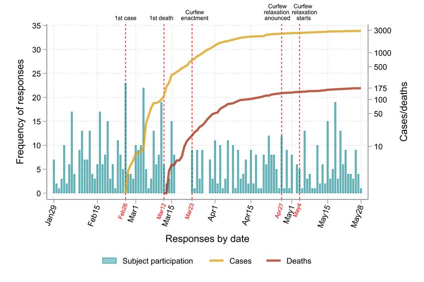
1       Introduction
    Economic theory suggests that a broad set of decisions relating to important outcomes such
as savings, investments, insurance, retirement plans, occupational choices, labor supply, health
services purchase, health behaviors and other aspects of everyday life, can be explained by
differences in agents’ budget constraints as well as Risk and Time Preferences (RTPs). RTPs
are at the crux of consumer behavior and in standard economic analysis, individual preferences
are considered to be stable over time. Andersen et al. (2008b) argue that the assumption of
stable preferences lies in the ability to assign causation between changing opportunity sets and
choices in comparative statics exercises or, in Stigler and Becker’s (1977) words, ‘no significant
behavior has been illuminated by assumptions of differences in tastes’.
    The assumption of stability of RTPs has been challenged however by the empirical literature.
For example, Chuang and Schechter (2015) find weak evidence of stability in experimental
measures of time preferences, although they find strong evidence of non-stability of experimental
measures of risk preferences over time. Schildberg-Hörisch (2018) take the view that the extent
to which preferences are stable is ultimately an empirical question. It is therefore of great
importance for the study of economic outcomes to understand whether RTPs are a stable
individual characteristic, change over time, or whether they are affected by various negative
shocks, such as financial crises, trauma from conflict, natural disasters or a pandemic.
    Our study adds to a stream of literature that examines the effect of major negative shocks
on peoples preferences.1 A large portion of the studies we are aware of examine the effect
of natural disasters on RTPs. Results from these studies point to contradictory results with
respect to risk. Some studies find an increase in risk seeking behavior due to a natural disaster.
For example, Eckel et al. (2009) investigated risk preferences of a sample of hurricane Katrina
evacuees shortly after evacuation, another sample of evacuees a year later, and a third sample
of residents with demographics similar to the Katrina evacuees. Women in the Katrina sample
shortly after evacuation were found to be significantly more risk loving than other samples.
Page et al. (2014) found that homeowners, who were victims of the 2011 Australian floods in
Brisbane and faced large losses in property values, were more likely to opt for risky gambles.
Hanaoka et al. (2018) investigated individuals’ risk preferences after experiencing the 2011 Great
East Japan Earthquake and found no effect for females, while males that were exposed to higher
intensities of the earthquake become more risk tolerant one year after the earthquake. Moreover,
this effect was persistent even five years after the earthquake.
    1
      Our study is also related to the stream of research that examines the intertemporal stability of RTPs. A
literature review of this research stream can be found in Drichoutis and Vassilopoulos (2016). Moreover, there
is a strand of research that examines the effect of major early life experiences on risk preferences. For example,
Bellucci et al. (2020) show that warfare exposure during childhood in the World War II was associated with
lower financial risk taking in later life. Moreover, Bellucci et al. (2020) review the literature on similar studies
that track and associate major early life experiences with preferences.

                                                         2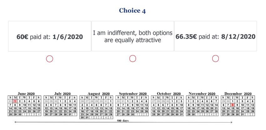
On the other hand, Cameron and Shah (2015) found that individuals who suffered a flood
or earthquake in rural Indonesia exhibited more risk-aversion as a consequence of increased
background risk perception of a future disaster. Similarly, Cassar et al. (2017) found that the
2004 tsunami in Thailand led to substantial and long-lasting increases in risk aversion as well
as in impatience. More recently, Beine et al. (2020) examined how two large earthquakes that
shook the Tirana area in Albania affected RTPs and found unambiguous effects towards more
risk aversion and impatience for affected individuals. Moreover, the second earthquake amplified
the effect of the first one, suggesting that experiences accumulate in their influence on RTPs.
Finally, Callen (2015) found that exposure to the Indian Ocean Earthquake tsunami increased
patience in a sample of Sri Lankan wage workers.
    A related stream of research examines the effect of conflict and violence on RTPs. Voors
et al. (2012) used a series of field experiments in rural Burundi to examine the impact of exposure
to conflict on RTPs. They found that individuals exposed to violence were more risk-seeking
and had higher discount rates. Callen et al. (2014) studied preferences in Afghanistan and
found that individuals exposed to violence, when primed to recall fear, exhibited an increased
preference for certainty. We are aware of only one study that examined the effect of a financial
crisis on RTPs. Jetter et al. (2020) found that males (but not females) were systematically more
sensitive to local economic conditions (e.g., their region’s unemployment rate) since the global
financial crisis of 2008.
    Our study focuses on the negative shock of the COVID-19 pandemic (caused by SARS-CoV-
2) which has been extremely disruptive to public health and the global economy. We originally
set up our study in 2017 with the purpose of administering, on an annual basis, a battery of in-
centivized and unincentivized measures to the student population of the Agricultural University
of Athens, Greece. Each year since 2017, we administered the exact same battery of measures to
students of the university that had voluntarily enrolled to participate in surveys/experiments.
Students were invited to participate online via Qualtrics and were invited to participate in
batches in order to achieve a good spread of responses across the one and a half month that the
elicitation took place. The original purpose of the study was to elicit a battery of psychologi-
cal, behavioral and economic measures and traits that could be later matched with data from
laboratory experiments conducted at the premises of the university. The study was initiated
in 2017 and was then repeated annually at similar dates every year. About halfway the 2020
wave, our study was re-designed due to the COVID-19 pandemic. The first case of COVID-19
was confirmed on February 26 in the country and on March 12 the first death occurred which
coincided with the end of the originally planned study for 2020.
    We decided to re-launch our study and invite back all subjects that had participated in the
2019 and the early 2020 wave. The re-launch of the study on March 23, 2020 coincided with
a general curfew imposed by the government banning all nonessential transport and movement

                                                3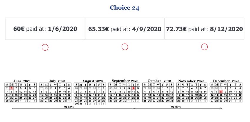
across the country. We extended the duration of the study until a few weeks after the opening
up of the economy and restart of business activity. Thus, for a considerable number of subjects
(we have more than 1,000 responses over the three waves), we have their response before the
pandemic, during the pandemic, and after successfully flattening the curve of cases/deaths.
    Our study adds to the emerging stream of studies that examine how risk or time preferences
have evolved over the course of the pandemic. Angrisani et al. (2020) study the stability of risk
preferences by comparing choices in the Bomb Risk Elicitation Task (Crosetto and Filippin,
2012) from undergraduate students (60 subjects) as well as professional traders and portfolio
managers (48 subjects) in London. They elicited subjects’ choices before the pandemic in 2019
as well as on a specific 13-day time window in April 2020 when London was in a lock-down.
They find no change in risk preferences during the pandemic.
    Bu et al. (2020) recruited 257 graduate students from Wuhan University of Science and
Technology in China (which was ground zero of the COVID-19 pandemic) before the pandemic.
They then administered a follow up online survey, and captured precise geolocation information
from subjects. Out of 225 subjects that responded in the follow up study, 106 were in provinces
outside of Hubei, with lower infection cases than Hubei. Subjects in all waves responded to
two general (hypothetical) risk preferences questions (that were used to form a composite scale)
while subjects amidst the pandemic were asked to answer a different (hypothetical) question
about how to allocate money to a hypothetical risky investment that had an equal probability of
higher returns or a loss. They found that subjects who were quarantined in Wuhan, with greater
exposure to the virus, allocated significantly less money to the risky investment option relative
to those in other cities within the Hubei province and those in other provinces of China. With
respect to the pre-pandemic period, subjects showed a large decrease in general preferences
for risk albeit there was no difference between areas with different intensity of exposure to the
pandemic.
    Ikeda et al. (2020) administered a five-wave internet panel survey to Japanese respondents
from March 13 to June 15, 2020 ( 4000 subjects/wave; N=14,470 for the balanced panel;
N=19,737 across the five waves). In the same time period the number of infected individuals rose
sharply in Japan. They elicited responses from two hypothetical questions where participants
were asked to choose the highest acceptable insurance premium from a given multiple price list
to cover the probabilistic risk of losing an amount of money. They used the stated insurance
premiums to calculate two prospect theory parameters for risk and the probability weighting
function and found that risk premiums decreased almost monotonically, implying that subjects
became more risk tolerant on average.
    Shachat et al. (2020) administered incentivized lottery choice tasks in the gain and loss
domain in 396 students from the Wuhan University, that were equally split among five waves
(79 subjects/wave). Data for each wave were collected right after key events starting in January

                                               4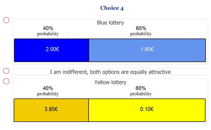
2020 and up to March 2020 (when WHO declared it a global pandemic) and were also contrasted
to pre-pandemic data from May, 2019. They observed significant increases in risk tolerance (risk
is measured based on the switching point) during the early stages of the COVID-19 crisis.
    Lohmann et al. (2020) administered incentivized lottery choice tasks, incentivized convex
time budgets and hypothetical investment games (investments that offered higher returns as
well as chances of losing the investment) to student subjects from Beijing universities. Subjects
participated in online surveys in October 2019 (wave 1), December 2019 (wave 2) and March
2020 (wave 3). In the third wave, subjects had been geographically scattered in various areas of
China and Lohmann et al. (2020) use the balanced sample of 539 subjects along with information
about virus exposure in the geographical region of subjects’ area to examine potential effects
on preferences. They find no significant changes in either risk or time preferences across waves.
    Table 1 summarizes the attributes of the various studies in this literature and compares these
with our study. One unique feature of our study is that in each wave, we collected responses
for a period longer than one and a half months, allowing us to record multiple key events in
the timeline of the pandemic. Moreover, our study is unique in that we jointly estimate the
structural parameters for various theories of risk and time preferences. Given that most studies
are focused on samples from China and only one of them measures time preferences, our study
is the only one providing structural estimates for time preferences for subjects from Europe.
Furthermore, our sample size is fairly large for an incentivized study, and using students as our
workhorse is not at odds with what almost all other studies cited in Table 1 did. Snowberg
and Yariv (2020) compare a sample from almost the entire undergraduate population of the
California Institute of Technology with a representative sample of the U.S. population and an
Amazon Mechanical Turk sample. They find that the student population exhibits less noise
as compared to the other samples and while large differences in behaviors are observed, these
differences had limited impacts on comparative statics and correlations between behaviors.

                                                5
Table 1: Literature on risk and time preferences in relation to the COVID-19 pandemic
Risk elicitation Measure for risk Incentives Type of subjects Sample size Subjects’ location When and how Results
Angrisani et al. (2020) Bomb Risk Elicitation Number of boxes opened Real incentives Undergraduate stu- Pre-pandemic: 79 students, London, UK Pre-pandemic (February- No change in risk preferences
Task in the BRET dents 56 traders/managers March 2019; lab experi-
Professional Amidst pandemic: 60 stu- ment)
traders/managers dents, 48 traders/managers April 9-21, 2020 (online)
(sub-sample of pre-
pandemic subejcts)
Bu et al. (2020) General Risk taking Weighted scale of two Hypothetical Graduate students Pre-pandemic: 257 students Pre-pandemic: Pre-pandemic in 2019 (Oc- Subjects reduce risk taking in the
questions general risk taking mea- Amidst pandemic: 225 stu- Wuhan, China tober 16- 18, 2019; paper pandemic but no effect between
Allocate money in sures (range from 1 to 5) dents (sub-sample of pre- Amidst pandemic: and pencil) areas with different intensity of
a 50:50 lottery with Amount of money allo- pandemic sample) 47% of subjects are February 28 - March 3, 2020 exposure to the pandemic
higher returns or cated to the investment outside of Hubei (online) Subjects in Wuhan (vs. Subjects
losses outside of Wuahn vs. Subjects
outside of Hubei), with greater
exposure to the pandemic, allo-
cate significantly less to the risky
gamble
Ikeda et al. (2020) Choose the highest in- Prospect theory parame- Hypothetical Stratified random 4000 subjects/wave Japan Five waves: March 13-16; As COVID-19 spreads, risk pre-
surance premium that ters are calculated sampling according (N=14,470 for the balanced March 27-30; April 10-13; miums decreased almost mono-
covers the probabilis- to age and gender panel; N=19,737 across the May 8-11; June 12-15, 2020 tonically, implying that subjects
tic risk of losing an distribution of the five waves) (online) became more risk tolerant on av-
6
amount of money Japanese census erage
Shachat et al. (2020) Lottery choice tasks in The switching point Real incentives Students Pre-pandemic: 206 subjects Wuhan, China Pre-pandemic: 206 sub- Increase in risk tolerance during
the gain and loss do- for the pairwise lottery Amidst pandemic: 79 sub- jects, May 2019 (online) the early stages of the pandemic
main ranges jects/wave (N=396 subjects January 24-26; February 4-
in total) 6; February 7-8; February
21-22; March 6-7, 2020 (on-
line)
Lohmann et al. (2020) Lottery choice task Coefficient of relative Real incentives ex- Students Pre-pandemic: 793 sub- Pre-pandemic: Bei- Pre-pandemic: October No significant changes in either
Convex time budget risk aversion midpoints cept for the Invest- jects (wave 1); 650 subjects jing universities 2019; December 2019 risk or time preferences across
Investment game (CRRA) ment game (wave 2) Amidst pandemic: ge- (online) waves
Percentage invested into Amidst pandemic: 539 sub- ographically dispersed Amidst pandemic: March
a lottery jects (wave 3) across country 2020 (online)
Dummy for present bi-
asedness parameter beta
being greater than 1
Discount rate (parameter
delta)
This study Lottery choice tasks Structural estimates of Real incentives Students Pre-pandemic: 304 subjects Greece Pre-pandemic: January 30 - No significant changes in risk or
Choices over time risk and time preferences (wave 1) March 20, 2019 (online) time preferences
dated monetary Amidst pandemic: 309 sub- Amidst pandemic: January
amounts jects (wave 2); 343 subjects 29 - March 16, 2020; March
(wave 3); N=359 for the bal- 23 - May 28, 2020 (online)
anced panelOur paper is structured as follows. In Section 2 we provide details about the design of
the study and elicitation of risk and time preferences. In the same section, we also provide
information about how the COVID-19 pandemic evolved in the country of our study (Greece)
as well as present how we go about with our structural econometric methods to model key
parameters from the theory of RTPs. Results and various robustness checks specifications are
presented in Section 3. We conclude and discuss our results in the last section.
2 Survey design
2.1 Sample and quality control
An online questionnaire was administered annually to the population of students registered in
the online recruitment software (ORSEE) of the university (Greiner, 2015), using the Qualtrics
platform. The first wave started in 2017 and invitations were sent out gradually on a rolling
basis, starting from late January to mid March. Similar days and dates were selected for the
next waves administered in years 2018, 2019 and 2020.2
Subjects could take the survey anytime they wanted once they received an invitation to
participate, but had a limited time window to complete the survey once they started. Figure 1a
shows the number of responses per day in the 2019 wave—one year before the outbreak of the
pandemic in the country. Similarly, Figure 1b shows responses per day for the 2020A wave
which was planned to conclude by March 17, 2020. As can be seen, halfway through the 2020A
wave, the first case of COVID-19 was confirmed (February 26, 2020) and the first death occurred
(March 12, 2020). Given the rapid development of subsequent cases and deaths, we decided
to launch an additional wave (2020B wave) where we invited the union of subjects that had
participated in the 2019 and 2020A waves to participate again. Our study was preregistered in
AsPredicted and a copy of the publicly available file can be found in the Electronic Supplemen-
tary Material. The start of the 2020B wave coincided with the enactment of a general curfew
(March 23, 2020) banning all nonessential transport and movement across the country. Invi-
tations to participate in the 2020B wave were distributed throughout the period of the curfew
(where cases and deaths increased) as well as for almost a month after the curfew was relaxed
(relaxation started on May 4, 2020) when the curve of cases and deaths had been flattened.
The recruiting procedure was similar for every wave and worked as follows. First, a list of
valid email addresses was compiled (along with names and surnames) using as source the list
of the universe of active students that are voluntarily registered through the ORSEE recruiting
system (Greiner, 2015). Email invitations were then sent in batches, scheduled for two times
2
The start of the survey was selected to be exactly 50 days from the payment of the sooner option of the
time preferences tasks that was always selected to be a working day (a Thursday) so that payments could be
delivered.
7a week, covering a period of approximately one and a half months. A reminder email was
sent two days after a batch of emails was first sent. Students are identified by their unique
student ID number and at the conclusion of the survey, they were asked to upload a picture of
their student ID for verification. Given that all waves included incentivized tasks of risk and
time preferences (described momentarily), money transactions were ordered only when their
ID was confirmed following a manual cross verification procedure by one of the investigators.
Moreover, the invitation email emphasized several times that the invitation link is unique and
that subjects must not forward their participation link to other subjects.3 Given that the
risk/time preferences tasks were part of a larger battery of questions and that subjects knew
they would be asked for verifiable data in order to be paid, it is unlikely that other subjects but
the intended recipients would answer a given questionnaire. Thus, we can be very confident that
subjects with a given ID number are the same subjects answering the questionnaire throughout
the different waves of the survey.
In total, we were able to collect 1103 responses over the three waves (2019, 2020A and 2020B).
Two responses were excluded because they were from a different person than the intended
recipient of the invitation email. Ninety responses were excluded because subjects stopped
the questionnaire before reaching the risk/time preferences elicitation tasks which renders them
useless for the purpose of the present paper. Three more persons were excluded because their age
or household size contained implausible values and their responses were deemed of ambiguous
quality. Table 2 shows the number of responses per wave as well as the number of unique
subjects that participated across one, two or all three waves. In all, we have 1008 response that
come from 495 unique subjects.
3
The general principle was that we excluded and did not pay a subject if their ID listed a different person
than the name we had sent the email to.
8Figure 1: Number of subjects per wave and day of the waves
(a) 2019 wave
(b) 2020 waves
Notes: The number of cases/deaths from COVID-19 are depicted in log scale.
9Table 2: Number of subjects per wave
Wave
Participated in . . . 2019 2020A 2020B Total
one wave 69 36 3 108
two waves 117 169 236 522
25 144
all three waves 126 126 126 378
Total 312 331 365 1,008
Notes: The numbers below the brackets indicate how subjects that participated in two waves are allocated
to the waves. For example, while 117 subjects from the 2019 wave participated in two waves, 25 of them also
responded in the 2020A wave. Similarly, of the 169 subjects that responded in two waves in the 2020A wave,
144 of them responded in the 2020B wave as well. It is implied that 92 subjects (=117-25 or =236-144)
participated in both the 2019 and 2020B waves.
2.2 The COVID-19 pandemic in Greece
The COVID-19 pandemic in Greece started with the first confirmed case on February 26,
2020, when a 38-year-old woman who had recently visited Milan, Italy, was confirmed to be
infected.4 Subsequent cases in late February and early March were related to a group of pilgrims
who had traveled to Israel and Egypt (and their contacts) as well as to persons who had traveled
to Italy.
The first death from COVID-19 occurred on March 12 in Greece. With subsequent cases
and deaths occurring at a faster rate, the government started imposing gradual restrictions
on movements and gatherings: all educational institutions were closed starting on March 11,
flights from Northern Italy (March 9) and the whole of Italy (March 14) were banned, borders
with Albania and North Macedonia were closed (March 16), and nonessential transport and
movement across the country was banned (March 23).5 During this period many businesses
and workplaces were also shutdown: theatres, hotels, courthouses, cinemas, shopping centres,
cafes, restaurants, bars, museums and archaeological sites, with the exception of supermarkets,
pharmacies and food outlets that were allowed to offer take-away and delivery only.
Following a successful flattening of the curve (see Figure 1b), the government announced on
April 27 a plan for the gradual lifting of the restrictive measures and the restart of business
activity. Starting on May 4, the curfew was relaxed and subjects did not need a special permit
to commute within their regional unit while retail-shops, coffee-places and restaurants gradually
4
The virus in Milan had spread through the Lombardy cluster of cases. The first cases were confirmed on
February 21 (Anzolin and Amante, 2020), but had been circulating undetected much earlier. It was subsequently
reported that the origin of these cases were connected to the first European local transmission that occurred in
Munich, Germany as early as January 19, 2020 (Luna, 2020).
5
Movement was permitted only for a pre-specified set of reasons: moving to and from work, grocery shopping,
visiting a doctor or assisting a person in need of help, exercising etc.
10Table 3: The Holt and Laury (2002) risk preference task
Lottery A Lottery B EVA e EVB e EV difference
p e p e p e p e
0.1 2 0.9 1.6 0.1 3.85 0.9 0.1 1.640 0.475 1.165
0.2 2 0.8 1.6 0.2 3.85 0.8 0.1 1.680 0.850 0.830
0.3 2 0.7 1.6 0.3 3.85 0.7 0.1 1.720 1.225 0.495
0.4 2 0.6 1.6 0.4 3.85 0.6 0.1 1.760 1.600 0.160
0.5 2 0.5 1.6 0.5 3.85 0.5 0.1 1.800 1.975 -0.175
0.6 2 0.4 1.6 0.6 3.85 0.4 0.1 1.840 2.350 -0.510
0.7 2 0.3 1.6 0.7 3.85 0.3 0.1 1.880 2.725 -0.845
0.8 2 0.2 1.6 0.8 3.85 0.2 0.1 1.920 3.100 -1.180
0.9 2 0.1 1.6 0.9 3.85 0.1 0.1 1.960 3.475 -1.515
1 2 0 1.6 1 3.85 0 0.1 2.000 3.850 -1.850
Notes: EV stands for Expected Value.
re-opened for business but with specific rules in place that they had to abide upon.
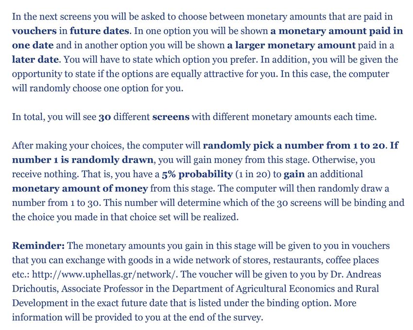
2.3 Incentivized elicitation of risk preferences
Subjects’ risk preferences were elicited using the Holt and Laury (2002) task (HL) as well
as a payoff varying task (PV). Drichoutis and Lusk (2016) have shown that greater predictive
performance of choices from a hold-out task can be achieved by combining information from the
HL task and a PV task. This is because the HL task varies the probabilities of the lottery choices
and provides a better approximation of the curvature of the probability weighting function (given
that subjects weigh probabilities non-linearly), while the PV task varies the monetary amounts
and is better in approximating the curvature of the utility function. In the HL task, individuals
are asked to make a series of 10 decisions between two lottery options (see Table 3). Table 4
shows a payoff varying task that keeps the probabilities constant across the 10 decision tasks
and instead changes the monetary payoffs across the 10 tasks. Both tasks are constructed in a
way that the expected value of lottery A exceeds the expected value of lottery B for the first
four decision tasks. Thus, a risk neutral person under Expected Utilty Theory (EUT) should
prefer lottery A for the first four decision tasks and then switch to lottery B for the remainder
of the decision tasks.
Choices were not presented all together in a table form, but each choice was presented
separately showing the probabilities and prizes as in Andersen et al. (2014).6 Subjects could
indicate whether they preferred lottery A, lottery B or whether they are indifferent between the
lotteries, in which case they were told that the computer would randomly decide the binding
6
It is likely that by presenting each pair of lotteries in a single screen allows subjects to focus more on a
specific pair of lotteries while when presenting all pairs of lotteries arrayed in a table makes subjects to think
the whole choice set as a single task.
11Table 4: The payoff varying risk preference task
Lottery A Lottery B EVA e EVB e EV difference
p e p e p e p e
0.5 1 0.5 1 0.5 1.2 0.5 0.2 1.00 0.70 0.300
0.5 1.2 0.5 1 0.5 1.5 0.5 0.2 1.10 0.85 0.250
0.5 1.4 0.5 1 0.5 1.8 0.5 0.2 1.20 1.00 0.200
0.5 1.6 0.5 1 0.5 2.2 0.5 0.2 1.30 1.20 0.100
0.5 1.8 0.5 1 0.5 2.9 0.5 0.2 1.40 1.55 -0.150
0.5 2.0 0.5 1 0.5 3.5 0.5 0.2 1.50 1.85 -0.350
0.5 2.2 0.5 1 0.5 4.6 0.5 0.2 1.60 2.40 -0.800
0.5 2.4 0.5 1 0.5 6.8 0.5 0.2 1.70 3.50 -1.800
0.5 2.6 0.5 1 0.5 9.2 0.5 0.2 1.80 4.70 -2.900
0.5 2.8 0.5 1 0.5 15 0.5 0.2 1.90 7.60 -5.700
Notes: EV stands for Expected Value.
lottery to determine their payouts. The order of appearance of the HL and PV tasks were
randomized across the subjects. An example of one of the decision tasks for the HL task is
shown in Figure 2 and the instructions for this task can be found in the Electronic Supplementary
Material in Section A.
For each subject, one of the choices was randomly chosen and paid out after we added a
e2 participation fee and we cross validated their student ID. Monetary payouts were paid via
bank transfer to subject’s preferred bank account.7 All transactions were ordered after cross
validation of their IDs was performed, which was normally within a few minutes after they
completed the questionnaire.
For a subset of observations (49 observations from 45 subjects), payments could not be
completed because subjects failed to complete the questionnaire and provide us with a valid
mobile phone number, although we do have their complete responses from the risk and time
preferences tasks.8 In addition, if a transaction would not go through, we would try to resend
the money for a maximum of two times or until we resolved the problem with the transaction
(in case the person would contact us to indicate there was a problem with the transaction).
For 82 observations coming from 76 subjects, transactions were not completed even though we
tried repeatedly to send the money. Finally, 877 transactions (87% of all observations) from 442
subjects were completed. Based on the 877 transactions, subjects were paid on average e4.4
(S.D.=2.62, min=2.1, max=17).9 We should note beforehand that our results are invariant
7
We used the ‘Pay a friend’ service of the bank ‘Eurobank’ which allows transferring money to subject’s
preferred bank account without knowing subject’s account number, only by using an email address or a mobile
phone number. The service is similar to the Zelle service operated by the Wells Fargo bank in the United States.
8
For the same reason, we don’t have complete demographic and attitudinal information for all subjects.
9
Note that because subjects repeatedly participated in the three waves, many of them were paid for more
than one time.
12Figure 2: Example screen for lottery choices
when using the full sample or just the constrained sample of subjects that accepted the payment.
Thus, this should alleviate any concerns that the subjects who did not accept the payment may
have treated the tasks as hypothetical and thus behaved differently.
2.4 Incentivized elicitation of time preferences
The experimental design for eliciting time preferences is based on the experiments of Coller
and Williams (1999), Harrison et al. (2002) and Andersen et al. (2008a). Subjects were con-
fronted with the payoff options listed in Table 5. In Table 5, option A (the principal) offers
either a e60 or a e90 sooner option. Option B offers an amount x 190 days later, where x
ranged from annual interests rates of 5% to 50% on the principal, compounded semi-annualy.
The sooner option (option A) was delivered on March 21 in the 2019 wave, March 19 in the
2020A wave, and June 1 on the 2020B wave.10 The later option (option B) was delivered 190
days later. These choices also offered the option of stating indifference between options, in which
case subjects knew that a random draw would decide the binding option. Another set of choices
also included a middle option which split the 190 days interval in two halves. Consequently, the
middle option was delivered 95 days later than option A. The purpose of the latter task was to
construct a choice set with fewer choices (choices 21 to 30 in Table 5) that is similar to choice
tasks 1 to 20 in Table 5. Comparison of these tasks is relegated to a different paper.
10
All dates and days were carefully pre-selected to be working days so that the payments could be physically
delivered to subjects.
13The tasks always impose a front-end delay on the early payment (option A) which comes
with two advantages. First, it avoids the passion for the present that decision makers exhibit
when offered monetary amounts today or in the future by holding the transaction costs of
future options constant (see Coller and Williams, 1999, for a discussion). Second, it allows us
to equalize the credibility of future payments because of the uncertainty associated with the
receipt of later rewards. Payments were promised to be paid with meal vouchers issued by
an international company, redeemable in a wide network of supermarkets, restaurants, coffees
shops etc in the country and all payments were guaranteed by a permanent faculty member (one
of the authors). Moreover, the faculty member has a long history of performing experiments in
this particular institution and is well known for paying students to participate in experiments.
Therefore, mistrust issues are expected to be minimal, if any. Subjects knew beforehand how
to contact the experimenter through telephone and email and where his office is located in the
campus. In all, subjects provided 30 choices for the time preference task that are used to infer
time preferences.
Financial constraints precluded us from paying every single subject; hence, subjects were
given a 5% chance of receiving any money from this task and they knew this beforehand. If a
subject was selected to receive money from this task, only one of their choices was selected as
binding and their choice was realized. Subjects were subsequently contacted by the experimenter
and were provided with details about when to receive their payment. All vouchers with the
corresponding amount that they had won, were delivered to subjects on exactly the date the
subject had selected for her respective choice.
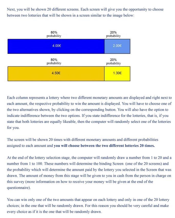
Experimental instructions for this task can be found in the Electronic Supplementary Mate-
rial in Section A. Figure 3 shows example screens for the times preferences choice task. Because
Read et al. (2005) document a date/delay effect; i.e., choices to be more patient when they are
described using calendar dates than when choices are characterized in terms of time delay from
the current moment, we used both dates and time delay to frame choices. Each choice always
displayed a calendar to illustrate the time delay and choices listed the delivery calendar dates
along with the monetary amount.
14Table 5: Payoff table in discount rate tasks
Payoff Middle Annual
Payment option A Payment option B
alternative payment option interest rate
1 60 A∼B 61.58 0.05
2 60 A∼B 63.17 0.10
3 60 A∼B 64.76 0.15
4 60 A∼B 66.35 0.20
5 60 A∼B 67.94 0.25
6 60 A∼B 69.54 0.30
7 60 A∼B 71.13 0.35
8 60 A∼B 72.73 0.40
9 60 A∼B 74.33 0.45
10 60 A∼B 75.94 0.50
11 90 A∼B 92.38 0.05
12 90 A∼B 94.76 0.10
13 90 A∼B 97.14 0.15
14 90 A∼B 99.53 0.20
15 90 A∼B 101.91 0.25
16 90 A∼B 104.31 0.30
17 90 A∼B 106.70 0.35
18 90 A∼B 109.10 0.40
19 90 A∼B 111.50 0.45
20 90 A∼B 113.90 0.50
21 60 60.79 63.17 0.05, 0.10
22 60 62.33 66.35 0.15, 0.20
23 60 63.85 69.54 0.25, 0.30
24 60 65.33 72.73 0.35, 0.40
25 60 66.78 75.94 0.45, 0.50
26 90 91.18 94.76 0.05, 0.10
27 90 93.50 99.53 0.15, 0.20
28 90 95.77 104.31 0.25, 0.30
29 90 98.00 109.10 0.35, 0.40
30 90 100.17 113.90 0.45, 0.50
Notes: The sooner option (option A) was delivered on March 21 in the 2019 wave, March 19 in the 2020A
wave and June 1 on the 2020B wave. The latter option (option B) was delivered 190 days later. The middle
option for the payoff alternatives 1 to 20 was an option of stating indifference between payment option A and
payment option B. The middle option monetary amount for the payoff alternatives 21 to 30, was delivered
95 days later than option A. In choices 21 to 30, the middle option is compounded with the smaller interest
rate of the two rates listed in the last column and the latter option is compounded with the largest interest
rate of the two rates listed in the last column.
15Figure 3: Example screen for time dated monetary choices
(a) Two options
(b) Three options
162.5 Theory and econometrics of risk and time preferences
Let the utility function be the constant relative risk aversion (CRRA) specification:
M 1−r
U (M ) = (1)
1−r
where r is the relative risk aversion (RRA) coefficient, r = 0 denotes risk neutral behavior,
r > 0 denotes risk averse behavior and r < 0 denotes risk loving behavior. If we assume that
Expected Utility Theory (EUT) describes subjects’ risk preferences, then the expected utility
of lottery i can be written as:
X
EUi = pi (Mj )U (Mj ) (2)
j=1,2
where p(Mj ) are the probabilities for each outcome Mj that are induced by the experimenter
(shown in Tables 3 and 4). A popular alternative is Rank Dependent Utility (RDU) developed by
Quiggin (1982). RDU extends the EUT model by allowing for non-linear probability weighting
associated with lottery outcomes.11 To calculate decision weights under RDU, we can replace
expected utility in equation (2) with:
X X
RDUi = wi [p(Mj )]U (Mj ) = wij U (Mj ) (3)
j=1,2 j=1,2
where wi2 = wi (p2 + p1 ) − wi (p1 ) = 1 − wi (p1 ) and wi1 = wi (p1 ) with outcomes ranked from
worst to best and w(·) is the probability weighting function.
There are many probability weighting functions that have been used in the literature and
here we consider two of the more popular ones that nest linear probabilities: a) Tversky and
pγ
Kahneman’s (1992) (TK) function w(p) = 1 (if γ = 1 it collapses to w(p) = p) and b)
(pγ +(1−p)γ ) γ
Prelec’s (1998) probability weighting function w(p) = exp(−(−lnp)ar ) where 0 < ar , 0 < p < 1
(if ar = 1 it collapses to w(p) = p).12
We assume subjects have some latent preferences over risk which are linked to observed
11
As in most experiments of choice under risk, our experiment involved multiple choices over lotteries for
which subjects where randomly paid for one of these choices. This payoff mechanism, known as the Random
Lottery Incentive Mechanism (RLIM), is incentive compatible if and only if the Independence Axiom holds
(Holt, 1986). Given that RDU does not include the independence axiom, then RLIM is inappropriate for non-
EUT theories on theoretical grounds. The use of the RLIM under non-EUT specifications either invokes the
assumption of the isolation effect i.e., that a subject views each choice in an experiment as independent of other
choices in the experiment or assumes two independence axioms as in Harrison and Swarthout (2021): one axiom
that applies to the evaluation of a given prospect which is assumed to be violated by RDU, and another axiom
that applies to the evaluation of the experimental payment protocol. Only the validity of the latter axiom is
required to ensure incentive compatibility of the RLIM.
12
Note, that the Prelec function is often applied with the constraint 0 < ar < 1 which requires that the
probability weighting function exhibits subproportionality (weighting function exhibits an inverse-S shape form).
We follow Andersen et al. (2018, 2014) and Harrison and Ng (2016) and use the more general specification from
Prelec (1998, Proposition 1: (C)), which only requires ar > 0 and nests the case where 0 < ar < 1.
17choices via a probabilistic model function of the general form:
(VB −VA )
!
RA C
P rB =Λ (4)
µ
where P r(B) is the probability of choosing lottery B (the right hand side lottery), µ is a
structural ‘noise parameter’ associated with the Fechner error story (sometimes called a scale or
precision parameter) used to allow some errors from the perspective of the deterministic model
and VA , VB are the decision-theoretic representations of values associated with lotteries A and
B i.e., Vk = EUk for k = A, B if the theory is EU or Vk = RDUk for k = A, B if the theory is
RDU. Λ(·) : R → [0, 1] is the standard logistic distribution function with Λ(ζ) = 1/(1 + e−ζ ),
Λ(0) = 0.5 and Λ(x) = 1 − Λ(−x), that is, Λ takes any argument between ±∞ and transforms
it to a number between 0 and 1 i.e., a probability.
C is a normalizing term that defines the heteroskedastic class of models.13 Wilcox (2008,
2011) proposed a ‘contextual utility’ error specification which adjusts the scale parameter by
C = Vmax − Vmin to account for the range of possible outcome utilities. C is defined as the
maximum utility Vmax over all prizes in a lottery pair minus the minimum utility Vmin over all
prizes in the same lottery pair. It changes from lottery pair to lottery pair, and thus it is said
to be contextual. Contextual utility maintains that the error specification is mediated by the
(VB −VA )
Vmax −Vmin
range of possible outcome utilities in a pair, so that P r(B) = Λ µ
.
With respect to time preferences, assume that EUT holds for choices over risky alternatives
and that discounting is exponential. Then a subject is indifferent between two income options
Mt and Mt+τ if and only if:
1
U (Mt ) = U (Mt+τ ) (5)
(1 + δ)τ
1
where DE (τ ) = (1+δ) τ is the discount factor for τ ≥ 0 and where the discount rate is
dE (τ ) = δ. The discount rate equalizes the present value of the two monetary outcomes in the
indifference condition (5). Under exponential discounting, the discount rate is stable over time.
Another class of discounting models is the family of hyperbolic specifications. A popular
hyperbolic specification is due to Mazur (1984) which specifies the discount factor as DH (τ ) =
1
(1+Kτ )
for some parameter K > 0 and discount rates dH (τ ) = (1 + Kτ )(1/τ ) − 1.
We can write the discounted utility of each option as:
MA1−r MB1−r
P VA = and P VB = D (6)
1−r 1−r
13
Note that this form of heteroskedasticity, refers to models where the standard deviation of utility dif-
ferences is conditioned on lottery pairs. Econometrically this can be considered as pair- and subject-specific
heteroskedasticity but one that requires no extra parameters into the model since the form of the heteroscedas-
ticity is determined by outcome utilities. See Wilcox (2008) for a related discussion.
18where D can be either the exponential DE or the hyperbolic discount factor DH . The probability
of choosing one of the options is given by:
D P VB − P VA
P rB =Λ (7)
ν
Given that some choice sets in the time preferences task presented subjects with choices
between three options i.e., a payment option A, a payment option B and a middle option C (see
Table 5), we can model the probability of choosing any of the three options using a multinomial
logit setup:
exp(P VJ /ν)
P rJD = PC for J = A, B, C (8)
j=A exp(P V j /ν)
This is a particularly attractive form as it is comparable with Equation 7 since for the case
D
= Λ P VB −P VA
= exp(P Vexp(P VB /ν)
of two options it can easily be shown that P rB ν A /ν)+exp(P VB /ν)
given
1
that Λ(ζ) = 1+e−ζ .
We can write the conditional log-likelihood for the risk preferences tasks as:
N
X
RA RA RA
lnL (r, µ; y, X) = (ln(P rB )|yi = 1) + (ln(1 − P rB )|yi = 0)
i=1 (9)
1 RA 1 RA
+( ln(P rB ) + ln(1 − P rB )|yi = −1)
2 2
where yi = 1, 0 denotes the choice of lottery B or A in the i th risk preference task, respectively,
and yi = −1 denotes the choice of indifference. X is a vector of variables that are assumed to
affect the estimated parameters. The conditional log-likelihood for the time preferences task
can be written as:
N
X
lnLD (T, ν; y, X) = D D
(ln(P rB )|yi = 1) + (ln(P rA )|yi = 0)
i=1 (10)
1 D 1 D
)|yi = −1) + (ln(P rCD )|yi = 2)
+( ln(P rA ) + ln(P rB
2 2
where yi = 1, 0 denotes the choice of option B (the later option) or A (the sooner option) in
the i th time preference task, respectively, yi = −1 denotes the choice of indifference and yi = 2
denotes the choice of the middle option C.14 X is a vector of variables that are assumed to
affect the estimated parameters. T is either δ under exponential discounting or K under the
hyperbolic specification.
14 D D
It is implied that for choice tasks 21 to 30, P rA and P rB are calculated based on Equation 8 and not
Equation 7.
19The joint likelihood of the risk aversion and discount rate responses can then be written as:
lnL(r, T, µ, ν; y, X) = lnLRA + lnLD (11)
Equation (11) is maximized using standard numerical methods. The statistical specifica-
tion also takes into account the multiple responses given by the same subject and allows for
correlation between responses by clustering standard errors; i.e., it relaxes the independence as-
sumption and requires only that the observations be independent across the clusters. The robust
estimator of variance that relaxes the assumption of independent observations involves a slight
modification of the robust (or sandwich) estimator of variance which requires independence
across all observations (StataCorp, 2013, pp. 312).
3 Results
Given competing theories of risk (EUT vs. RDU), the various probability weighting func-
tions, and discount factors, we utilize a model selection criteria that allow us to select one model
over another. We therefore estimated all possible combinations of risk and discount factors and
calculated the associated information criteria such as Akaike’s and Bayesian information crite-
ria (AIC and BIC). AIC and BIC do not reveal how well a model fits the data in an absolute
sense; i.e., there is no null hypothesis being tested. Nevertheless, these measures offer relative
comparisons between models on the basis of information lost from using a model to represent
the (unknown) true model.15
In order to explore the effect of the pandemic on risk and time preferences, we modeled the
structural parameters as a function of either a) wave dummies defined as dummies for the waves
2019 (pre-pandemic wave), 2020A and 2020B (see also Table 2) or b) event dummies defined as
key events that occurred in the timeline of the pandemic in the country. These events are: i)
first reported case in the country (February 26; overlaps with the 2020A wave), ii) first reported
death in the country (March 12; overlaps with the 2020A wave) iii) onset of curfew when all
nonessential transport and movements across the country were banned (March 23; coincides
with the beginning of the 2020B wave) iv) announcement of a plan for the gradual lifting of
the restrictive measures and the restart of business activity (April 27; overlaps with the 2020B
wave) and curfew relaxation and business re-openning (May 4; overlaps with the 2020B wave).16
Figure 1b shows a timeline of these events as well.
15
Drichoutis and Lusk (2016) have shown that AIC and BIC are in agreement in terms of model selection
with more complex selection criteria such as Vuong’s test (Vuong, 1989), Clarke’s test (Clarke, 2003) or the
out-of-sample log likelihood (OSLLF) criterion (Norwood et al., 2004).
16
Because the time between announcement of relaxation of the restrictive measures and the actual relaxation
was very short, we merged these two key events in one.
20Table 6 shows the AIC and BIC values for the various estimated models combining the
different risk and discount factor functions. The models are estimated with two different sets
of dummies as described above; i.e., wave dummies and event dummies.17 The two information
criteria do not fully agree with each other but do point that the hyperbolic discount factor
function performs better than the exponential. The disagreement between AIC and BIC is
whether a model with linear probabilities for risk fits the data better than a model with Prelec’s
(1998) probability weighting function. In what follows, we present both EUT and RDU models
(with Prelec’s (1998) probability weighting function) with a hyperbolic discount function, since
these are favored by the information criteria.
Table 6: Akaike’s and Bayesian Information criteria
with Wave dummies with Event dummies
Risk Discount Log-L AIC BIC Log-L AIC BIC
Linear Exponential -28472.86 56961.73 57031.93 -28461.96 56951.92 57074.77
Linear Hyperbolic -28423.46 56862.93 56933.13 -28412.41 56852.81 56975.66
T&K Exponential -28469.95 56961.89 57058.41 -28457.31 56954.63 57130.12
T&K Hyperbolic -28419.24 56860.49 56957.01 -28406.23 56852.45 57027.95
Prelec Exponential -28467.34 56956.69 57053.21 -28455.01 56950.01 57125.51
Prelec Hyperbolic -28414.37 56850.75 56947.27 -28401.50 56842.99 57018.49
Notes: Linear stands for linear probabilities which is equivalent to EUT; T&K stands for Tversky and
Kahneman’s (1992) probability weighting function; Prelec stands for Prelec’s (1998) probability weighting
function; Bold numbers indicate the lowest number column-wise, highlighting which model performs better
than other.
Table 7 shows the estimates of the structural parameters for EUT and RDU that are modeled
as a function of two sets of dummy variables. Models (1) and (2) use the wave dummies while
models (3) and (4) use the event dummies. As evident, none of the wave or event dummies are
statistically significant, indicating remarkable stability of estimated risk and time preference
parameters across time. The estimated parameters also allow us to test the RDU model versus
the EUT by testing whether the parameter ar in the probability weighting function w(p) =
exp(−(−lnp)ar ) is statistically different from 1.18 A joint significance test with respect to the
regressors of the ar parameter that a) the wave dummies in model (2) are 0 and the constant is
equal to 1, does not reject the null (χ2 = 3.50, p-value = 0.321), b) the event dummies in model
(4) are 0 and the constant is equal to 1, does not reject the null (χ2 = 4.97, p-value = 0.548),
indicating that EUT is a better descriptive model of subjects’ risk preferences.
17
Note that in the estimations of Table 6, we removed choices of 35 cases where subjects chose the dominated
option (i.e., the lottery offering a lower amount of money over certainties) in the last choice of the Holt and Laury
(2002) task. We also removed choices from 17 cases (associated with 11 unique subjects) where after geolocating
their IP addresses, we found they responded in the 2020A or the 2020B wave from abroad. This is because
living abroad at the time of the pandemic likely disassociates behavior with the key events that happened in
this period inside the country.
18
When ar = 1 then w(p) = p.
21Table 7: Structural estimates
EUT RDU EUT RDU
(1) (2) (3) (4)
r
Constant 0.542∗∗∗ (0.026) 0.506∗∗∗ (0.034) 0.542∗∗∗ (0.026) 0.506∗∗∗ (0.034)
2020A wave 0.032 (0.038) 0.016 (0.049)
2020B wave -0.023 (0.039) -0.027 (0.051)
2020 events:
Before first case 0.052 (0.045) 0.047 (0.057)
Before first death 0.024 (0.055) -0.000 (0.069)
Before curfew -0.056 (0.093) -0.105 (0.123)
Curfew starts 0.016 (0.048) -0.009 (0.061)
Curfew announced relaxation -0.069 (0.049) -0.050 (0.067)
αr
Constant 0.902∗∗∗ (0.055) 0.901∗∗∗ (0.055)
2020A wave -0.044 (0.078)
2020B wave -0.011 (0.083)
2020 events:
Before first case -0.013 (0.092)
Before first death -0.064 (0.105)
Before curfew -0.135 (0.179)
Curfew starts -0.070 (0.095)
Curfew announced relaxation 0.052 (0.113)
K
Constant 0.208∗∗∗ (0.015) 0.225∗∗∗ (0.018) 0.208∗∗∗ (0.015) 0.225∗∗∗ (0.018)
2020A wave -0.016 (0.021) -0.008 (0.026)
2020B wave 0.030 (0.023) 0.034 (0.029)
2020 events:
Before first case -0.028 (0.024) -0.025 (0.029)
Before first death -0.008 (0.030) 0.004 (0.037)
Before curfew 0.027 (0.053) 0.052 (0.074)
Curfew starts 0.011 (0.029) 0.028 (0.036)
Curfew announced relaxation 0.052∗ (0.029) 0.043 (0.036)
µ 0.131∗∗∗ (0.003) 0.128∗∗∗ (0.003) 0.131∗∗∗ (0.003) 0.128∗∗∗ (0.003)
ν 0.067∗∗∗ (0.002) 0.066∗∗∗ (0.002) 0.067∗∗∗ (0.002) 0.066∗∗∗ (0.002)
N 47800 47800 47800 47800
Log-likelihood -28423.46 -28414.37 -28412.41 -28401.50
AIC 56862.927 56850.745 56852.811 56842.994
BIC 56933.125 56947.268 56975.658 57018.490
Notes: Standard errors in parentheses. * pThe results are similar if we constrain the sample to only those for which we have their data
for at least two waves (see Table A1 in the Electronic Supplementary Material) or to only those
for which we have their data for all three waves (see Table A2 in the Electronic Supplementary
Material) or to only those that the electronic payment transaction went through after the end
of the experiment (see Table A3 in the Electronic Supplementary Material).
Another way to augment the models of Table 7 is by including variables related to the
perception of the pandemic or attitudes, and coping with it. We first constructed measures of
the number of deaths and cases at the level of administrative regions of the country, adjusted
for the population size (i.e., number of deaths and cases were divided by the population size of
the respective region). We achieved this by matching IP (Internet Protocol) address geolocation
data with the number of recorded deaths and cases in the respective administrative region the
day each subject responded.19 Naturally, these measures take a value of zero for dates before the
onset of the pandemic. Table A4 in the Electronic Supplementary Material shows that the vast
majority of responses (> 90%) originated from the cities of Athens/Piraeus and Thessaloniki
which account for roughly 40% of the population in the country.
Models (1) and (2) in Table 8 show the structural parameter estimates when adding a gender
dummy and the cases/deaths variables in the models for EUT and RDU, respectively. Models
(3) and (4) constrain the sample to the 2020B wave and augment the set of regressors for the
structural parameters with a set of variables from questions that where included in the last
wave, in order to capture attitudes and behavior with respect to the pandemic.20
As evident in Table 8, none of the variables of interest has a statistically significant effect.
Although some variables are shown to be statistically significant in the RDU models, note that
19
We queried the recorded IP addresses collected by Qualtrics with http://ip-api.com which is an appli-
cation programming interface that allows to query IP addresses and returns back location data at the level of
region/city in the country. The number of deaths/cases per day and per region is maintained and curated by
iMEdD’s (Incubator for Media Education and Development) content production division. iMEdD is a non profit
organization founded with a donation of Stavros Niarchos Foundation with a mission to support and promote the
transparency, credibility and independence in journalism on the grounds of securing meritocracy and excellence in
the field. The data can be found in iMEdD’s GitHub repository: https://github.com/iMEdD-Lab/open-data.
20
The set of variables includes: a) dummies about perception of how effective social distancing is with possible
answers being i) very inefficient or inefficient, ii) neither inefficient, nor efficient, iii) efficient iv) very efficient, b)
a dummy about whether the respondent has family members or others in their inner circle considered a high risk
group, c) a composite score variable capturing whether respondents are stressed about the pandemic situation.
This composite score variable was constructed as the sum of five variables that respondents answered on a five
Likert scale ranging from ‘highly disagree’ to ‘highly agree’: i) I’m nervous/stressed ii) I’m calm/relaxed (reverse
coded) iii) I worry about my health iv) I worry about the health of members of my family v) I feel stressed
when I have to leave home, d) a composite variable capturing whether respondents’ tendency to attribute the
virus or the pandemic in conspiracy theories or misconceptions about the virus. This composite score variable
was constructed as the sum of five variables that respondents answered on a five Likert scale ranging from ‘very
unlikely’ to ‘very likely’: i) Coronavirus was made in a lab in China, got out of control and transmitted to
the population ii) Coronavirus was made in a US lab and US soldiers then infected the population in China
iii) Coronavirus is a zoonosis that spread from animals to humans (reverse coded) iv) Coronavirus is no more
dangerous than common flu v) Coronavirus was invented as a pretense for limiting personal liberties.
23You can also read