OPEN SOURCE CONE-BEAM RECONSTRUCTOR - OSCAR
←
→
Page content transcription
If your browser does not render page correctly, please read the page content below
OSCaR:
       Open Source Cone-beam Reconstructor
             Nargol Rezvani∗(1), D. A. Aruliah (2),
            John M. Boone (3), Michael J. Flynn (4)
        Kenneth R. Hoffmann (5), Kenneth R. Jackson (1),
            Douglas Moseley (6), Xiaochuan Pan (7),
           Jeffrey Siewerdsen (8), Xiangyang Tang (9)

1. Dept. of Computer Science,               2. Faculty of Science, Univ. of ON
Univ. of Toronto, Bahen 4239,               Inst. of Tech., 2000 Simcoe St. N.,
40 St. George St., Toronto, ON,             Science Bldg UA4000, Oshawa, ON,
M5S 2E4, CANADA.                            L1H 7K4, CANADA.

3. Dept. of Radiology, UC Davis             4. Dept. of Radiology, Henry Ford
Medical Center, 4860 Y Street,              Health Sys., Radiology Research 2F,
Suite 3100, Ellison ACC Bldg,               1 Ford Pl, Detroit, MI, 48202, USA.
Sacramento, CA, 95817, USA.

5. Neurosurgery Dept., Toshiba              6. Dept. of Radiation Therapy Phys.,
Stroke Research Center, Univ. of            Princess Margaret Hospital,
Buffalo, 455 Biomed. Research Bldg,         610 University Ave, Toronto, ON,
Buffalo, NY, 14214-3025, USA.               M5G 2M9, CANADA.

7. Dept. of Radiology, Univ. of             8. Dept. of Biomedical Eng.,
Chicago, MC-2026,                           Johns Hopkins Univ., Traylor Bldg 718,
5841 S Maryland Ave.,                       720 Rutland Ave., Baltimore,
Chicago, IL, 60637, USA.                    MD, 21205, USA.

9. Dept. of Radiology, Emory Univ.,
Winship Cancer Inst., 1701 Uppergate Dr.,
Suite C5018, Atlanta, GA, 30322, USA.

 ∗

                                      1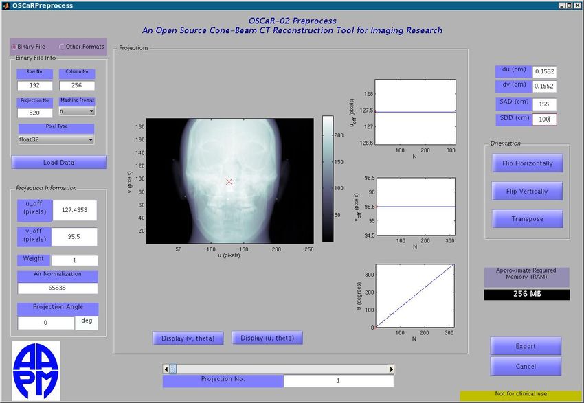
Abstract

        OSCaR (Open Source Cone-beam Reconstructor) is a software pack-

    age developed for computing three-dimensional reconstructions from data

    gathered from cone-beam x-ray CT scanning geometries. The package

    is implemented in Matlab with the intention of being easy to use and

    portable across many computer architectures. The code is intended for

    research use, not clinical or commercial implementation. OSCaR is not in-

    tended to be fast; it is meant to be transparent, so that researchers can

    examine the source code and easily understand and extend the underlying

    algorithms. The code includes a GUI (Graphical User Interface), as well

    as a small library of Matlab functions that can be customized and in-

    corporated into users’ own implementations. The downloadable package

    contains the OSCaR software, this document, a shorter tutorial document,

    sample data sets to illustrate the features of OSCaR, comments from the

    beta testers, and two posters in which OSCaR was presented at scientific

    meetings.

Contents

1 Introduction                                                                     4

  1.1   Assumptions and Limitations . . . . . . . . . . . . . . . . . . . .         5

2 Running OSCaR                                                                    7

  2.1   The GUI OSCaRMain . . . . . . . . . . . . . . . . . . . . . . . . .        7

  2.2   The GUI OSCaRPreprocess . . . . . . . . . . . . . . . . . . . . .          7

        2.2.1   Geometry/Resolution Parameters . . . . . . . . . . . . . .         9

        2.2.2   Storage Parameters     . . . . . . . . . . . . . . . . . . . . .    9

        2.2.3   Projection-Dependent Parameters . . . . . . . . . . . . .          11

        2.2.4   Orientation Buttons . . . . . . . . . . . . . . . . . . . . .      12

                                        2
2.2.5   Export to OSCaRReconstruct . . . . . . . . . . . . . . . .         12

  2.3   The GUI OSCaRReconstruct . . . . . . . . . . . . . . . . . . . .           12

        2.3.1   Reconstruction Size . . . . . . . . . . . . . . . . . . . . .      13

        2.3.2   Filter . . . . . . . . . . . . . . . . . . . . . . . . . . . . .   15

        2.3.3   Execute and Export . . . . . . . . . . . . . . . . . . . . .       16

  2.4   The Function OSCaR . . . . . . . . . . . . . . . . . . . . . . . . .       17

        2.4.1   Syntax . . . . . . . . . . . . . . . . . . . . . . . . . . . . .   18

3 One Quick Example                                                                19

  3.1   Running the GUI OSCaRPreprocess . . . . . . . . . . . . . . . .            19

  3.2   Running the GUI OSCaRReconstruct . . . . . . . . . . . . . . . .           20

  3.3   Running the Function OSCaR . . . . . . . . . . . . . . . . . . . .         21

4 Standalone Executable                                                            22

5 Conclusions                                                                      23

6 Acknowledgements                                                                 24

                                         3
1 Introduction
OSCaR (Open Source Cone-beam Reconstructor) is a software package written in
Matlab developed for generating 3D reconstructions from x-ray data acquired
from cone-beam scanning geometries. It is based on the Feldkamp-Davis-Kress
(FDK) algorithm [3], for 3D cone-beam CT (CBCT) reconstruction. The lack
of practical, flexible, free FDK software implementations can hamper medical
physics researchers and inhibit multi-institutional research collaboration. Rec-
ognizing the need for common, referenceable imaging research software, OS-
CaR was developed as a research tool for free distribution by the American
Association for Physicists in Medicine (AAPM). The goal is to offer a straight-
forward, open source code and GUI (Graphical User Interface) implementation
that emphasizes flexibility, generality, and ease of use. The implementation has
a transparent interface for 3D image reconstruction with the intention of pro-
viding a useful base platform for developing advanced techniques (e.g., artifact
correction) or for conducting image quality studies (e.g., selection of optimal re-
construction filters). The code is intended for research use, not clinical or com-
mercial implementation. Although compiled software is certainly faster than
interpreted Matlab code, a Matlab implementation circumvents the neces-
sity of custom compiled libraries. The intention is not to produce the fastest
implementation; rather, it is to provide code from which researchers can start
developing their own algorithms.
Broadly speaking, OSCaR has three main components: pre-processing, re-
construction, and export. In the pre-processing stage, CBCT data is parsed
from a broad, general base of standard data-file formats, accessible to Matlab
(e.g., DICOM, binary, JPEG, TIFF, PNG, etc.). The source-detector pair is
assumed to move in a circular path, but OSCaR can allow for variation in the
position of the piercing point as a function of the projection angle. Parameters
4associated with geometric corrections, sampling, air normalization, and other
device-dependent properties that affect acquisition of the sinogram data can be
specified using the pre-processing GUI prior to reconstruction.
In the reconstruction stage, OSCaR permits the specification of the Field-Of-
View (FOV), voxel size and reconstruction filters. The actual voxel-driven re-
construction uses the well-known FDK filtered back-projection algorithm. Then,
in the export stage, the reconstructed data can be saved as a three dimensional
matrix, which can be exported as a standard data-file, such as DICOM, binary,
etc, and visualized.
In accordance with the desires of the AAPM Research Subcommittee, OS-
CaR is made freely available on the AAPM web-site to members of the AAPM
for research in algorithm development, CBCT image quality studies, and multi-
institutional collaboration.
1.1 Assumptions and Limitations
The following assumptions and general recommendations are pertinent to the
use and further development of OSCaR:
1. The geometry for acquisition of the 3D sinogram is circular (i.e., the
source-axis-distance and the source-detector-distance are constant). No
detector tilt is allowed. However, the code does allow variations in the
location of piercing points (u0 , v0 ) from view to view.
2. The projection geometry involves a point x-ray source with a divergent
x-ray beam.
3. The detector is flat and has rectangular detector elements of uniform di-
mensions.
4. The projections may be collected at non-uniform projection angles.
55. Measurement distances are in centimeters unless otherwise stated.
6. The origin of a pixel is its centre.
7. OSCaR does not handle Parker weights. The code handles projection sets
covering exactly 180 + fan or 360 degrees. Anything in between is im-
properly weighted.
8. OSCaR has been tested on Matlab 2009a with the Image Processing Tool-
box 6.2.
9. Potential file formats for input projection data can be any image file format
accessible to Matlab (e.g., DICOM, jpg, tiff, etc). Alternatively, all
projections can be input in a single binary data file.
10. Sinogram data stored in binary files are ordered in column major order
(consistent with the Matlab convention).
11. Loading/saving data from three-dimensional arrays can take some time
depending on the memory available on the computer and disk-access time.
If a read or write seems to be taking a long time, please be patient; the
GUI has likely not crashed; there is no “hourglass” cursor icon in the
initial release to indicate that the code is “busy”.
The largest 3D sinogram that can be loaded by OSCaR depends on the amount
of memory available on the computer. The entire 3D sinogram must fit into
memory with pixel values stored as double precision floating point numbers.
Given that a single projection of 192 by 256 pixels needs about 400 KB of mem-
ory, 300 projections require about 113 MB. Conversely, 1 GB of free accessible
memory corresponds to 320 (192 × 256 pixel) projections. Similar restrictions
apply to the memory required for reconstructions; the user must be able to store
6at least double the memory required for the user-specified reconstruction array
(for work arrays and the like).
2 Running OSCaR
Prior to launching OSCaR, the directory containing the source code for OS-
CaR must be in your Matlab path. Also, a .csv (comma-separated value,
see Section 2.2.3) file needs to be prepared, and stored in the same directory
that contains the 3D sinogram projections. The requirements are outlined in
Section 2.2.3 below.
The user has two options for using OSCaR. The first option is invoked by
calling OSCaRMain which launches a GUI. The GUI OSCaRMain provides access
to two other GUIs, OSCaRPreprocess and OSCaRReconstruct. The second
option for using OSCaR is entirely command-line based and is invoked using
OSCaR with appropriate inputs.
2.1 The GUI OSCaRMain
OSCaRMain (shown in Figure 1) is the primary GUI. The buttons can be used to
launch OSCaRPreprocess and OSCaRReconstruct or to cancel the computation.
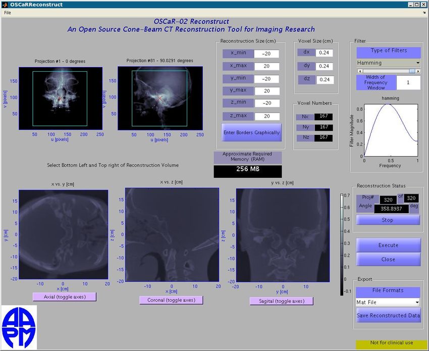
2.2 The GUI OSCaRPreprocess
The GUI OSCaRPreprocess (shown in Figure 2) is used to input the 3D sinogram
data for processing prior to reconstruction. The user can initiate the GUI OS-
CaRPreprocess
• by clicking the button Load Projections from the GUI OSCaRMain, or
• by entering OSCaRPreprocess at the Matlab command prompt.
7Figure 1: OSCaRMain
The individual projections are assumed to have been captured at Nproj dif-
ferent gantry angles. Each projection consists of an image of resolution Nu × Nv
pixels. The v-direction on the detector is assumed to be parallel to the axis of
revolution of the source-detector pair; the u-direction on the detector is assumed
to be perpendicular to the v-direction.
Prior to loading the Nu × Nv × Nproj values comprising the 3D sinogram
from disk, the user must provide some information about how the data was
collected and how the data is stored. Although some of it can be entered into
the GUI OSCaRPreprocess directly, some of this information can vary for each
of the Nproj projections.
8As such, before loading the 3D sinogram into memory, OSCaRPreprocess re-
quires the following information from the user:
1. geometry/resolution parameters (pertaining to all the projections);
2. storage parameters (pertaining to all the projections); and
3. projection-dependent parameters.
The details of how the user can provide this information follows.
2.2.1 Geometry/Resolution Parameters
These are the parameters that describe the geometry and resolution of the
cone-beam apparatus used to acquire the projection data. These parameters
are summarized as follows:
du Pixel length (cm) in u direction (perpendicular to axis)
dv Pixel length (cm) in v direction (parallel to axis)
.
SAD Source-Axis-Distance (cm)
SDD Source-Detector-Distance (cm)
The GUI OSCaRPreprocess has textboxes on the right-hand side that allow
users to specify each of du, dv, SAD, and SDD appropriately.
2.2.2 Storage Parameters
The projection data is assumed to be stored in one of two generic ways:
1. The Nproj projections are all stored in a single binary data file in column
major order.
2. The projections are stored in Nproj individual image files, each of which
is in some format that Matlab can import (e.g., JPEG, TIFF, DICOM,
etc.).
9The GUI OSCaRPreprocess has a pair of radio-buttons at the top left corner
(Binary File versus Other Formats, see Figure 2) to specify the choice of data
format.
If the user selects Binary File, all the Nproj projections are assumed to be
stored in a single file in column-major order (the filename should be provided
in the .csv file, see Section 2.2.3). As such, the user must edit the textboxes to
provide the Row No. (i.e., Nu ), the Column No. (i.e., Nv ), and the Projection
No. (i.e., Nproj ). The user also needs to specify, using pull-down menus, the
Pixel Type (int32, float32, etc.) and the Machine Format required for reading
the binary data. Strings describing the machine formats are summarized below.
n Numeric format of machine on which Matlab is running (default)
b 32 bit IEEE floats with big-endian byte ordering
l 32 bit IEEE floats with little-endian byte ordering
s 64 bit IEEE floats with big-endian byte ordering
a 64 bit IEEE floats with little-endian byte ordering
d VAX D floats and VAX ordering
g VAX G floats and VAX ordering
If the user selects Other Formats, the Nproj projections are assumed to be
stored in Nproj individual image files (whose names are provided in the .csv
file, see Section 2.2.3). In this case, the values of Nu and Nv can be inferred
directly from the image files as they are loaded (recall that the values of Nu and
Nv must be the same for every projection).
After input parameters N u, N v, Nproj and the input file format are specified,
an estimate of the amount of memory required is displayed in the box “Approx-
imate Required Memory (RAM)”, on the right side of the GUI. The user can
check whether the machine has enough memory to run OSCaRPreprocess. For
example, to process SampleData.csv and 20070611-1-roc-750434170.img,
use the following values:
10Nproj 320
Nrow 192
Ncol 256
du 0.1552
dv 0.1552
SAD 100
SDD 155
2.2.3 Projection-Dependent Parameters
Certain parameters can vary from projection to projection. These should be
specified by the user in a .csv (comma separated values) file to avoid having to
enter each parameter into a textbox in the GUI OSCaRPreprocess. A .csv file
can be prepared and exported using most commonly-used spreadsheet programs.
The user is prompted for the name of the .csv file before the 3D sinogram can
be loaded into memory.
The .csv file should consist of Nproj rows, each with 6 columns. The 6
columns of the kth row of the .csv file consist of information pertinent to the
kth projection (k = 1 : Nproj ). These columns are as follows:
filename θG uoff voff I0 w .
filename string naming file in which kth projection is stored
θG gantry angle of kth projection (degrees)
uoff offset of centre of detector perpendicular to axis (cm)
.
voff offset of centre of detector parallel to axis (cm)
I0 air normalisation (same units as values in projections)
w weight (dimensionless)
An example of such a .csv file is included in this package.
112.2.4 Orientation Buttons
In the orientation box on the right side of the GUI, three buttons, Flip Horizon-
tally, Flip Vertically, and Transpose, can be found. Assuming the data coming
from the scanner is stored in the matrix P , pushing one of these buttons results
in one of the following operations performed on P :
1. Flip Horizontally
2. Flip Vertically
3. Transpose
The modified data is displayed in the GUI. Once a suitable orientation is found,
the user can save the projection data and export it to the reconstruction com-
ponent, OSCaRReconstruct.
2.2.5 Export to OSCaRReconstruct
When the user has completed the preprocessing stage described above, the data
can be exported to a .mat file1 that can be used in the reconstruction stage
(OSCaRReconstruct). The .mat file consists of a structure, experiment, with
two fields: param and data. The first field, in turn, consists of fourteen subfields
that are filled by the values displayed in the GUI OSCaRPreprocess; the second
one, as its name suggests, contains the data from the scanner.
2.3 The GUI OSCaRReconstruct
The GUI OSCaRReconstruct (shown in Figure 3) is used for image reconstruc-
tion. The user can initiate the GUI OSCaRReconstruct
• by clicking the button Reconstruct from the GUI OSCaRMain, or
1A .mat file is a a file which contains saved variables written in a Matlab specific format.
12Figure 2: OSCaRPreprocess
• by entering OSCaRReconstruct at the Matlab command prompt.
Once OSCaRReconstruct is launched, the user must load the .mat file produced
in the previous stage by OSCaRPreprocess.
2.3.1 Reconstruction Size
The user is required to specify the box [xmin , xmax ], [ymin , ymax ] and [zmin , zmax ]
that bounds the voxelized reconstruction either graphically or numerically. These
values provide the dimensions of the reconstruction domain in the real world.
If the user enters the reconstruction sizes incorrectly (e.g., out of range or the
minimum value is greater than the maximum value), an error message appears.
1. Graphically: After pushing the button Enter the Borders Graphically, the
13Figure 3: OSCaRReconstruct
user must click on the images to select the bottom left and top right of the
reconstruction volume. (In total two points on each image are required)
2. Numerically: The user must enter the borders numerically.
The default values yield a two dimensional axial reconstructed slice. An estimate
of the amount of memory needed for reconstruction is displayed in a box near the
centre of GUI with the title “Approximate Required Memory (RAM)”. The user
should verify that the machine has enough memory to run OSCaRReconstruct.
142.3.2 Filter
The next step is selecting the appropriate filter with a desired width of frequency
window (between 0 and 1). On the right side of the GUI OSCaRReconstruct, a
drop down menu offers a selection of different filters, such as Ram-Lak, Shepp-
Logan, Cosine, Hamming, and Hann. These filters are defined in the function
OSCaRFilter.m. This function returns a vector of coefficients that is multiplied
element-wise by the rows of the Fourier transform of the sinogram data. This
vector of coefficients is our filter. The input arguments of OSCaRFilter are
the length and the spatial resolution of the projection data, and the fraction of
frequencies below the Nyquist frequency which we want to pass. The latter is
a value between zero and one. The user must enter the width of the frequency
either in the edit box or by using the slider on the right side of the OSCaRRe-
construct GUI.
In OSCaRFilter the filters are defined as a multiplication of the ramp filter
by the following apodizing windows:
• Shepp-Logan: sinc(x) ,
• Cosine: cos(x) ,
• Hamming: 0.54 + 0.46 cos(x),
• Hann: 0.5 + 0.5 cos(x).
Alternatively, the user may choose to enter their own apodizing window, by
choosing “new filter” in the drop down menu on the right. After selecting this
option, the user is asked to enter the apodizing window as a function of x. Note
that here x is a vector. As an example, the user can enter cos(x) or cos(x). ∗
sin(x) . (Note the array element-wise multiplication operator “.*”, since x is a
vector.) If the function is not recognized by Matlab, an error message alerts
the user; otherwise, the corresponding filter (the apodizing window multiplied
15by the ramp filter) is displayed and is used in the reconstruction. If the user
chooses “No Filter”, then the function returns an empty vector.
In the filtering part of OSCaR, scaling of time and frequency domains are
computed according to reciprocity relations as in [1].
2.3.3 Execute and Export
Pressing the “Execute” button on the right side of the GUI starts the reconstruc-
tion process using the function OSCaRFDK.m. This function uses the Feldkamp-
Davis-Kress (FDK) algorithm [3, 12].
• After fixing the projection angle, OSCaRFDK returns the value calculated
by the FDK algorithm for each voxel. Then the program loops over the
projection angles, and the calculated values by OSCaRFDK are summed
together;
• the OSCaRFDK routine uses the nearest neighbour interpolation to find the
detector coordinates (u, v) that are closest to the projections of voxels
(x, y, z);
• we have vectorized the FDK algorithm to increase the computational
speed.
When the reconstruction is complete, the user can save the reconstructed data
and the parameters defining the FOV (Field-of-View) of the reconstructed vol-
ume in three ways:
1. Save the reconstructed data in a .mat file. The user can specify a name for
the .mat file, but the reconstructed data (P ), and the parameters defining
the FOV of the reconstructed volume, (xmin, xmax, ymin, ymax, zmin, zmax),
are saved in a structure called Save data, with seven fields. To open the
16.mat file (reconstructed data), the user can use the following command in
Matlab.
>> load(’NameofMatFile.mat’);
>> Save_data
Save_data =
P: [167x167x167 double]
xmax: 20
xmin: -20
ymax: 20
ymin: -20
zmax: 20
zmin: -20
2. Save the reconstructed data as a binary file and the needed parameters,
such as the reconstruction borders and voxel sizes, in a text file.
3. Save the reconstructed data as DICOM files.
2.4 The Function OSCaR
This function opens a .mat file that stores preprocessed projection data as
created by OSCaRPreprocess. The function OSCaR can then be used to perform
FDK reconstruction. By setting the value of verbose to 1 or 0, the user may
choose to have the reconstructed volumes (axial, sagital, and coronal) displayed,
or not, respectively. The function OSCaR returns the reconstruction as its output.
172.4.1 Syntax
OSCaR(FileName,’PropertyName’,PropertyValue)
where,
• FileName:: String.
“FileName” is the name of the .mat file to be loaded as built by OSCaR-
Preprocess. This file contains a structure named experiment, with two
fields, param and data. The first field has the subfields: projf ilenames , θ ,
uof f , vof f , I0 , weights, Nproj , Nrow , Ncol , du , dv , SAD , SDD , and
IAD , and the second field has the projection data.
• PropertyName and PropertyValue:
PropertyName PropertyValue Default
FilterName ’No filter’,’hamming’, ’hann’, No filter
’cosine’, ’shepp-logan’, ’ram-lak’
ReconstructionVolume Vector of length 6 Entered Graphically
(xMin,xMax,yMin, · · · ,
yMax,zMin,zMax)
VoxelSize Vector of length 3 (dx,dy,dz) Determined Internally .
by using a
geometry-dependent
formula
FilterWidth Width of Frequency Window 1
(Real value between 0 and 1)
Verbose 0 or 1 1
Note that to enter the borders graphically, the user must select bottom left
and top right corners of the reconstruction volume.
183 One Quick Example
In this section, we give an example of how to run OSCaR. Prior to launching OS-
CaR, the directory containing the source code for OSCaR must be in your Matlab
path. As mentioned in the previous sections, OSCaR has three GUIs: OSCaRMain,
OSCaRPreprocess, and OSCaRReconstruct. In the following subsections simple
examples of how to use each of these GUIs are provided. Then an example of
how to use the function OSCaR is presented.
To start, enter OSCaRMain at the Matlab command prompt. The buttons
in this GUI, Load Projections and Reconstruct, can be used to initiate OSCaR-
Preprocess and OSCaRReconstruct, respectively (see Figure 1). These two
GUIs can also be launched from the command line directly.
3.1 Running the GUI OSCaRPreprocess
As mentioned above, this GUI can be launched either from the Matlab com-
mand line, or by pressing the button Load Projections in the OSCaRMain GUI.
1. The GUI OSCaRPreprocess has a pair of radio-buttons at the top left
corner for a choice of Binary File versus Other Formats to specify one of
these choices. Choose the radio-button Binary File, and enter the following
values in the box underneath the radio-buttons (see Figure 2).
Nproj 320
Nrow 192
Ncol 256
Machine Format n
Pixel Type float32
2. Press Load Data and open 20070611-1-roc-750434170.img and SampleData.csv
in the examples folder. At this time, the images are displayed. The user
19can fix the orientation of the images by using the buttons on the left
side, Flip Horizontally, Flip Vertically, and Transpose. In this case, use
Transpose and Flip Vertically to get the correct orientation.
3. Enter the following values in the textboxes on the right side of the GUI:
du 0.1552
dv 0.1552
SAD 100
SDD 155
4. The user can update the values in the projection information box, but, in
this example, do not change those values.
5. Press the Export button, choose a name for a .mat file, e.g. SampleData.mat.
As a result, all the preprocessed projection data and the data entered into
the GUI OSCaRPreprocess is saved in the .mat file.
3.2 Running the GUI OSCaRReconstruct
As mentioned above, this GUI can be launched either from the Matlab com-
mand line or by pressing the button Reconstruct on OSCaRMain.
1. After launching the GUI OSCaRReconstruct, the user must pick a .mat
file, possibly produced by OSCaRPreprocess in the previous stage, e.g.
SampleData.mat.
2. Enter the reconstruction size either numerically or graphically, by pushing
the button Enter the Borders Graphically, and then clicking on the images
to select the bottom left and top right of the reconstruction volume (in
total two points on each image are required). The values can be changed
manually from the boxes provided in the box Reconstruction Size (see
Figure 3).
203. Select the appropriate filter with the desired width of frequency window,
which is between 0 and 1. The user may choose to enter their own filter, by
choosing “new filter” in the drop down menu on the right as a function of x,
e.g. cos(x) or cos(x). ∗ sin(x) . (Note the array element-wise multiplication
operator “.*” is used, since x is a vector.)
4. Press the Execute button to start the reconstruction. This stage may take
a few minutes, depending on the size of the reconstruction.
5. When the reconstruction is complete, the reconstructed volume can be
saved in one of three ways:
(a) Save the reconstructed data in a .mat file. With this option, the data
is stored in binary form (not human-readable).
(b) Save the reconstructed data as a binary file. The other parameters
(FOV, voxel sizes, etc.) should be stored in a text file.
(c) Save the reconstructed data as DICOM files.
3.3 Running the Function OSCaR
As explained in Subsection 2.4, this function opens a .mat file, which contains
information about the projections and the data coming from the detector stored
in a structure. After filtering and using the FDK algorithm, it returns the
reconstruction.
The syntax of this function is
OSCaR(FileName,’PropertyName’,PropertyValue),
where the FileName is a string that provides the name of the .mat file to be
loaded. This file contains a structure named experiment, with two fields, param
and data. This file can be built by OSCaRPreprocess, e.g. SampleData.mat.
21Example
M = OSCaR(’examples/SampleData.mat’,’FilterName’,’hamming’,
’ReconstructionVolume’,[-15,15,-15,15,0,0],’Verbose’,0)
Note that to enter the borders graphically, the user must select bottom left
and top right corners of the reconstruction volume.
4 Standalone Executable
In the OSCaR package, we have also included a Windows executable version of
the GUIs called OSCaREXE. The standalone application OSCaREXE is generated
by the Matlab compiler and can be found in the exe folder. The application
OSCaREXE can be run on any Windows machine even if Matlab is not installed.
The user must ensure that the correct version of the Matlab Compiler
Runtime (MCR) environment is installed on the target machine. We have used
Matlab 2008b, which uses MCR version 7.9. The MCR installer is included in
this package in the exe folder. The user may already have the MCR installed
on their machine. To verify the version number of the installed MCR, type the
following command at the Matlab command prompt:
[mcrmajor, mcrminor] = mcrversion
If the user does not have Matlab or the correct version of the MCR installer
installed on their computer, then they can run MCRInstaller in the exe folder.
After installing the MCR, to run the standalone executable, the user must
launch OSCaREXE in the exe folder. This loads the GUI OSCaRMain and the user
can proceed to follow the steps described in the previous sections.
225 Conclusions
In this note, we presented OSCaR, a software package written in Matlab, based
on the FDK algorithm. This software is developed for generating 3D reconstruc-
tions from x-ray data acquired from cone-beam scanning geometries. OSCaR is
intended to be flexible, easy-to-use, and portable across many computer ar-
chitectures. The code is intended for research use, not clinical or commercial
implementation. OSCaR is meant to be transparent, rather than being fast. Our
goal is for the underlying algorithms to be easy to understand so that users can
readily modify and extend the source code to test new techniques.
In this report, we explained how different components of OSCaR can be used
and what features they have. We included several examples to help users learn
how to work with OSCaR. We also mentioned several assumptions and limitations
in OSCaR, so that users know what to expect from this package. Since OSCaR is an
open-source package, users can customize the code, and incorporate it in their
own algorithms. For example, OSCaR can be used as a basis for comparison with
algebraic reconstruction techniques. With suitable modifications to account
for Parker weights, OSCaR could also be used in 4DCT studies to compensate
for motion-induced artifacts in sinograms. OSCaR could also be used for filter
selection studies or to develop and compare models for correcting for beam
hardening.
In accordance with the desires of the AAPM Research Subcommittee, OS-
CaR is made freely available on the AAPM web-site to members of the AAPM
for research in algorithm development, CBCT image quality studies, and multi-
institutional collaboration.
236 Acknowledgements
This work was supported in part by the American Association of Physicists
in Medicine (AAPM), the Natural Sciences and Engineering Research Council
(NSERC) of Canada, and Mathematics of Information Technology and Complex
Systems (MITACS) Canadian research network.
References
[1] William L. Briggs and Van Emden Henson, The DFT: An Owners’ Man-
ual for the Discrete Fourier Transform, Society of Industrial and Applied
Mathematics (SIAM), 1995.
[2] Charles L. Epstein, Introduction to the Mathematics of Medical Imaging,
Prentice Hall, Upper Saddle River, N.J., 2003.
[3] L. A. Feldkamp, L. C. Davis, and J. W. Kress, Practical Cone-beam Algo-
rithm, J. Opt. Soc. Amer. A, 1(6):612-619, Jun 1984.
[4] R. W. Hamming, Digital Filters, Prentice Hall, Englewood Cliffs, N.J.,
1989.
[5] Avinash C. Kak and Malcolm Slaney, Principles of Computerized Tomo-
graphic Imaging. Society of Industrial and Applied Mathematics (SIAM),
Philadelphia, 2001.
[6] F. Natterer and Frank Wubbeling, Mathematical Methods in Image Recon-
struction, Society of Industrial and Applied Mathematics (SIAM), Philadel-
phia, 2001.
24[7] T. Rodet, F. Noo, M. Defrise, The Cone-Beam Algorithm of Feldkamp,
Davis, and Kress Preserves Oblique Line Integrals, Medical Physics 31,
1972, 2004.
[8] B. Rust and D. Donnelly, The Fast Fourier Transform for Experimentalists,
Part I: Concepts, Computing in Science & Eng., vol. 7, no. 6, 2005, pp.
85-90
[9] B. Rust and D. Donnelly, The Fast Fourier Transform for Experimentalists,
Part V: Filters, Computing in Science & Eng., vol. 7, no. 6, pp. 85-90, 2005.
[10] Henrik Turbell, Cone-Beam Reconstruction Using Filtered Back-projection,
PhD thesis, 2001.
[11] James S. Walker, Fast Fourier Transforms, Second Edition, CRC-Press,
1996.
[12] S. Webb, A Modified Convolution Reconstruction Technique For Divergent
Beams, Phys. Med. Bio, 1982, Vol 27, No. 3, 419-423.
[13] Yuchuan Wei, Ge Wang, and Jiang Hsieh, An Intuitive Discussion on the
Ideal Ramp Filter in Computed Tomography, Comput. Math. Appl., 49(5-
6):731-740, 2005.
25You can also read