Optimal Control of Oscillation Timing and Entrainment Using Large Magnitude Inputs: An Adaptive Phase-Amplitude-Coordinate-Based Approach
←
→
Page content transcription
If your browser does not render page correctly, please read the page content below
Optimal Control of Oscillation Timing and Entrainment Using
                                                            Large Magnitude Inputs: An Adaptive
                                                         Phase-Amplitude-Coordinate-Based Approach
                                                                                              Dan Wilson1
arXiv:2102.04535v1 [math.DS] 8 Feb 2021

                                              1
                                                  Department of Electrical Engineering and Computer Science, University of Tennessee,
                                                                              Knoxville, TN 37996, USA

                                                                                          February 10, 2021

                                                                                                Abstract
                                                        Given the high dimensionality and underlying complexity of many oscillatory dynamical
                                                    systems, phase reduction is often an imperative first step in control applications where oscillation
                                                    timing and entrainment are of interest. Unfortunately, most phase reduction frameworks place
                                                    restrictive limitations on the magnitude of allowable inputs, limiting the practical utility of the
                                                    resulting phase reduced models in many situations. In this work, motivated by the search for
                                                    control strategies to hasten recovery from jet-lag caused by rapid travel through multiple time
                                                    zones, the efficacy of the recently developed adaptive phase-amplitude reduction is considered for
                                                    manipulating oscillation timing in the presence of a large magnitude entraining stimulus. The
                                                    adaptive phase-amplitude reduced equations allow for a numerically tractable optimal control
                                                    formulation and the associated optimal stimuli significantly outperform those resulting from
                                                    from previously proposed optimal control formulations. Additionally, a data-driven technique
                                                    to identify the necessary terms of the adaptive phase-amplitude reduction is proposed and
                                                    validated using a model describing the aggregate oscillations of a large population of coupled
                                                    limit cycle oscillators. Such data-driven model reduction algorithms are essential in situations
                                                    where the underlying model equations are either unreliable or unavailable.

                                          1        Introduction
                                          Mathematical analysis and control of oscillatory dynamical systems is a widely studied problem
                                          with relevant applications to neurological brain rhythms [37], [20], [26], circadian physiology [11],
                                          [3], [48], and various other physical and chemical systems [50], [13], [45], [62], [66]. Given the high
                                          dimensionality and sheer complexity of many oscillatory dynamical systems, model reduction is
                                          often a necessary first step in their analysis. While many reduction strategies have been developed
                                          for limit cycle oscillators, phase reduction [64], [14], [27] is one of the most widely applied techniques
                                          which allows for oscillatory systems of the form

                                                                                            ẋ = F (x) + U (t),                                            (1)

                                          where x ∈ RN is the system state, F describes the nominal dynamics, and U is an exogenous input
                                          to be analyzed according to
                                                                                θ̇ = ω + Z(θ) · U (t),                                (2)

                                                                                                     1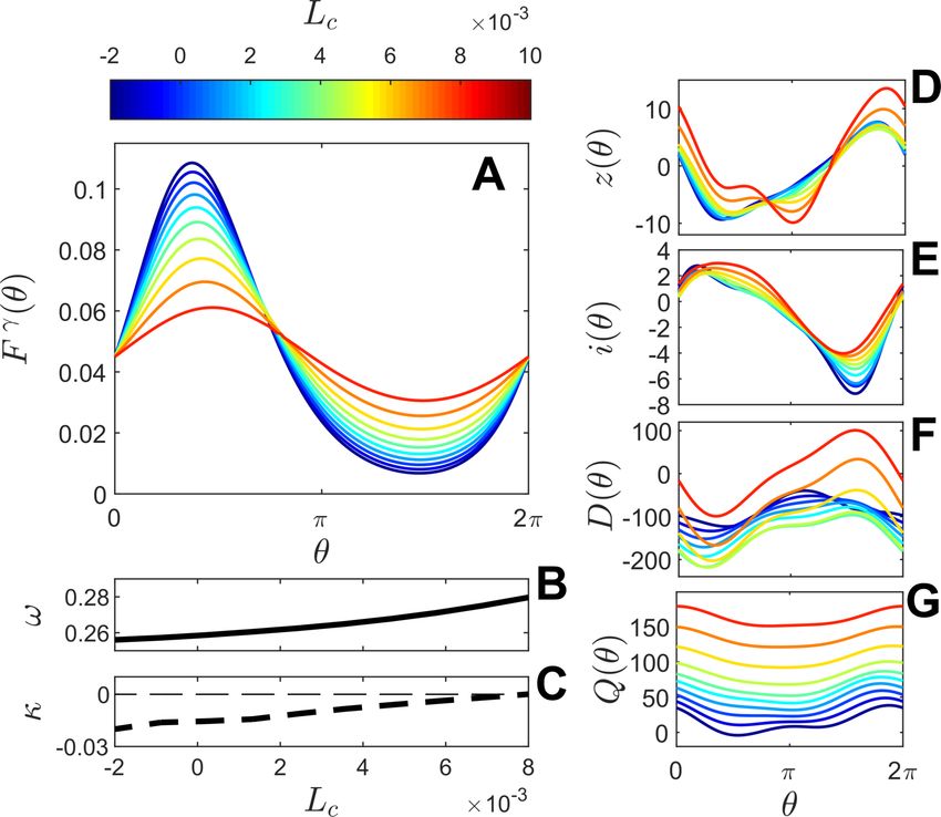
where the phase θ ∈ [0, 2π) characterizes the state of the oscillator in reference to a limit cycle,
ω(p0 ) = 2π/T is the natural frequency where T is the nominal, unperturbed period, Z(θ) is the
phase response curve (i.e., the gradient of the phase coordinate evaluated on the limit cycle),
and the ‘dot’ denotes the dot product. Phase reduction provides a tremendous decrease in the
dimensionality of a given limit cycle oscillator, allowing for the original N -dimensional, generally
nonlinear behavior to be studied as a 1-dimensional ordinary differential equation. In exchange
for this tremendous reduction in dimensionality, the magnitude of the perturbations is required to
be uniformly bounded in time by , where 0 <   1 to ensure that Equation (2) is valid to first
order accuracy in . Practically, the reduction (2) can be applied to make predictions about system
behavior in response to larger magnitude inputs with the understanding that its performance will
begin to degrade as the magnitude of the input becomes larger; precise bounds on the allowable
U (t) are usually not known a priori and vary on an application-by-application basis.
     In an effort to extend the applicability of phase reduction when larger magnitude inputs are
considered, a variety of reduction algorithms have been proposed that take into account the transient
dynamics in directions transverse to the periodic orbit. For example, the notions of entrainment
maps [11], operational phase coordinates [59], functional phase response curves [9], local orthogonal
rectification [29], stochastic phase [5], and average isophase [47] rely on different definitions of
‘phase’, with each being well-suited for specific applications. Other recent works have attempted to
use phase-amplitude coordinate systems to identify reduced order equations that are valid beyond
first order accuracy in , [58], [16], [57], [44], [61]. While such techniques generally provide better
results than comparable first order accurate reduction methods, they still suffer from limitations
that preclude the consideration of medium-to-large magnitude inputs. Koopman analysis is an
emerging reduction framework that can be used to represent a nonlinear dynamical oscillator (or
more generally any nonlinear dynamical system) with a linear, but infinite dimensional operator
[7], [33], [22]. However, it can be difficult to identify a suitable finite dimensional basis that fully
captures the dynamics of the Koopman operator.
     Recently, an adaptive phase-amplitude reduction strategy was proposed in [54] that uses the
standard definition of asymptotic phase based on isochrons [64], [18] and also considers the slowly
decaying isostable coordinates [63] which represent level sets of the slowest decaying Koopman
eigenfunctions [32]. By considering a family of limit cycles that emerge for different parameter sets,
the nominal parameter set can be adaptively chosen in order to limit the error in the reduced order
equations. As shown in [54], provided the Floquet exponents of the truncated isostable coordinates
are O(1/) terms, the adaptive phase-amplitude reduction is valid to O() accuracy even when the
input U (t) is an O(1) term.
     Because the adaptive phase-amplitude reduction framework allows for the consideration of par-
ticularly large magnitude inputs, this reduction framework is an attractive candidate for control
of oscillation timing in situations where the application of large magnitude inputs is unavoidable.
In this work, optimal control of oscillation timing in the presence of a large magnitude entraining
stimulus will be considered. This situation can be used to represent circadian rhythms that are
entrained to a 24-hour light-dark cycle. In humans, a population of roughly 10,000 coupled neu-
rons referred to as the suprachiasmatic nucleus is responsible for maintaining circadian time [36],
[43]. The body’s circadian cycle is nominally entrained to a 24-hour light-dark cycle in order to
regulate sleep and wake timing among other physiological processes. Circadian misalignment, more
commonly referred to as jet-lag, represents a disruption to this nominal steady entrainment and
results from a mismatch between the environmental time and one’s own circadian clock [46].
     Numerical models of circadian oscillations have been helpful for developing post-travel treatment
protocols to aid in recovery from circadian misalignment [3], [48], [10], however, optimal control
algorithms can typically only be implemented on in simplified, low-dimensional models. For more

                                                   2
complicated and high-dimensional models, standard phase reduction techniques typically fail. There
are two fundamental reasons for this: the first is that circadian rhythms result from the collective
oscillation of a large number of coupled oscillators. Phase reduction methods can be used for these
population oscillations using techniques described in [25], [30], [23] and [15], however, the inter-
oscillator coupling usually results in amplitude coordinates that decay slowly. Practically, these
amplitude coordinates represent shifts in the distribution of phases of the individual oscillators;
without the ability to accurately account for these time-varying phase distributions only particularly
small magnitude inputs can be considered. The second difficulty that arises when using phase
reduction methods for applications involving circadian oscillations is that the nominal 24-hour
light-dark cycle itself is generally be considered a strong perturbation that shifts the oscillator state
far from its nominal limit cycle [12]. For all but a small subset of oscillator models with dynamics
that can be greatly simplified when certain assumptions are made [27], [39], it is difficult to predict
how the aggregate behavior will respond to the large magnitude entraining stimuli precluding the
consideration of control inputs to manipulate the phase. For these reasons, reduction techniques
that allow for large inputs are essential for applications that involve circadian oscillations.
    There are two primary focal points of this work. The first is the development and assessment of
strategies to implement the adaptive phase-amplitude reduction in an optimal control framework
to manipulate oscillation timing and speed recovery from circadian misalignment. In the results to
follow, by making appropriate assumptions about the characteristics of the adaptive reduction, a
calculus of variations approach can be used to identify optimal control inputs in the presence of a
large magnitude entraining stimulus. This strategy can be used to identify inputs that engender
significantly larger time shifts than other recently proposed oscillation timing control frameworks.
The secondary focus of this work is the development of data-driven techniques for identification of
the necessary terms of the adaptive phase-amplitude reduction that are valid in situations where
numerical models are either unreliable or unavailable. By leveraging techniques developed in [56]
a general strategy is proposed to accurately determine necessary terms of the adaptive reduction
solely from observable data.
    The organization of this paper is as follows: Section 2 gives necessary background information
about the adaptive phase-amplitude reduction method used to identify reduced order models in
this work. Section 3 considers an optimal control formulation using the adaptive phase-amplitude
reduction for manipulation of oscillation timing in the presence of an external entraining stimulus.
Analogous, previously proposed formulations are also considered that use phase-only and first
order accurate phase-amplitude reductions in order to provide comparisons with the proposed
optimal control formulation. Section 4 provides results for the optimal control framework when
using a relatively simple, three-dimensional model of circadian oscillations. Section 5 considers
a population-level model of coupled oscillators that give rise to a collective oscillation. Here, a
strategy is presented for identifying the necessary terms of the adaptive reduction from a single
system observable and the optimal control strategy is subsequently implement to identify efficient
stimuli to hasten recovery from circadian misalignment. Section 6 provides concluding remarks.

2    Background
In the analysis to follow, a phase reduction (2) will be considered that explicitly incorporates a set
of nominal parameters. In this context, consider an ordinary differential equation of the form
                                         ẋ = F (x, p0 ) + U (t),                                    (3)
where x, F , and U are defined identically to the terms from (1) and p0 ∈ RM is a set of nominal
parameters. Suppose that for a constant choice of p0 , (3) has a stable periodic orbit xγp0 . Provided

                                                    3
that U (t) is sufficiently small, phase reduction is a well established technique [14], [27], [64] that
can be used to analyze the behavior of (3) in the weakly perturbed limit according to
θ̇ = ω(p0 ) + Z(θ, p0 ) · U (t), (4)
where ω and Z are defined identically to the terms from (2).
2.1 Isostable Coordinate Reduced Frameworks
In situations where larger magnitude inputs must be considered, phase reduction can still be used
but one must also consider the transient dynamics in directions transverse to the limit cycle. Various
phase-amplitude coordinate frameworks have been developed for this purpose [58], [49], [53], [29],
[5], [59], [44]; this work will focus on strategies that use isostable coordinates to characterize the
amplitude coordinates [32], [58], which represent level sets of the slowest decaying eigenfunctions
of the Koopman operator [32]. Each isostable coordinate represents the magnitude of a particular
Koopman eigenmode. Intuitively, states that correspond to larger magnitude isostable coordinates
will take longer to decay to the periodic orbit. For the slowest decaying Koopman eigenfunctions,
explicit definitions can be given for the isostable coordinates in the basin of attraction of a fixed point
[32] or periodic orbit [58], however, faster decaying isostable coordinates must be defined implicitly
according to their respective Koopman eigenfunctions with decay rates that are governed by their
associated Floquet exponents. Previous work [63] (cf. [8]) investigated strategies for computing the
behavior of the isostable coordinates for models of the form (3) in response to perturbations in a
neighborhood of the limit cycle yielding reduced order equations of the form
θ̇ = ω(p0 ) + Z(θ, p0 ) · U (t),
ψ˙j = κj (p0 )ψj + Ij (θ, p0 ) · U (t),
β
X
x(θ, ψ1 , . . . , ψβ ) = xγp0 (θ) + g k (θ)ψj ,
k=1
j = 1, . . . , β, (5)
where ψj is the j th isostable coordinate with corresponding Floquet exponent κj , g k (θ) are as-
sociated Floquet eigenfunctions, and Ij (θ, p0 ) is the isostable response curve that represents the
gradient of the isostable coordinates evaluated on the periodic orbit. In (5), the rapidly decaying
amplitude coordinates are generally truncated so that only β ≤ N − 1 of the slowest decaying
isostable coordinates are explicitly considered – isostables with rapid exponential decay can gen-
erally be assumed to be zero without adverse effects in the accuracy of the reduction. Numerical
computation of Z, and each Ij and g k can be performed using the ‘adjoint method’ [6] and related
equations described in [57]. The so-called ‘direct method’ [21], [38] and related data-driven tech-
niques [60], [56] have been developed for inferring the necessary terms of (5) from experimental
data when the underlying model equations are unknown.
Much like (4), Equation (5) is only valid provided the state remains sufficiently close to the
periodic orbit. Unlike (4) alone, however, (5) can be used to provide information about the tran-
sient behaviors that characterize the amplitude dynamics. It is generally assumed that under the
application of input with O() magnitude that each ψj remains an O(). In this case, (5) is valid to
leading order . Recent work has investigated isostable reduced equations that are valid to second
order accuracy [58], [60] and beyond [57], however, these reduction frameworks still require the
magnitude of the applied inputs to be sufficiently small. Other reduction frameworks have been de-
veloped that are valid for inputs with arbitrary magnitude provided that they are sufficiently slowly
4varying [28], [40] or rapidly varying [42], [52]. Nevertheless, few general reduction frameworks are
available that are valid for arbitrary, large magnitude inputs.
2.2 Adaptive Phase-Isostable Reduction
Isostable reduced equations of the form (5) typically assume that the nominal system parameters
are constant in the analysis of a perturbed limit cycle. Recent work [54] has leveraged the phase-
isostable coordinate reduction framework (5) to develop an adaptive reduction that actively sets
the nominal system parameters in an effort to keep isostable coordinates low, thereby allowing
for inputs without O() constraints (either in magnitude or rate of change). As discussed in [54],
to implement an adaptive phase-isostable reduction, first suppose that in some allowable range of
nominal system parameters p ∈ RM that xγp (t) is continuously differentiable with respect to both t
and p. One can then rewrite Equation (3) as
ẋ = F (x, p) + Ue (t, p, x), (6)
where
Ue (t, p, x) = U (t) + F (x, p0 ) − F (x, p). (7)
Intuitively, F (x, p) represents the underlying dynamics for a given choice of system parameters
p, and Ue represents the effective input. Allowing p to be variable, and assuming that θ(x, p) and
ψj (x, p) are continuously differentiable in a neighborhood of the limit cycle for all x and p, one can
transform (6) to phase and isostable coordinates via the chain rule
dθ ∂θ dx ∂θ dp
= · + · ,
dt ∂x dt ∂p dt
dψj ∂ψj dx ∂ψj dp
= · + · , (8)
dt ∂x dt ∂p dt
for j = 1, . . . , β. Above, provided that the state is close to the periodic orbit xγp , ∂x
∂θ
· dx
dt =
∂ψj dx
ω(p) + Z(θ, p) · U (t) and ∂x · dt = κj (p)ψj + Ij (θ, p) · U (t) as given by Equation (5). For the
remaining terms, as explained in [54], one can write
∂θ h iT
D(θ, p) ≡ = Z(θ, p) · ∂∆x∂p1
p
. . . Z(θ, p) ·
∂∆xp
∂pM ,
∂p
∂ψj h iT
Qj (θ, p) ≡ = Ij (θ, p) · ∂∆x
∂p1
p
. . . I j (θ, p) ·
∂∆xp
∂pM , (9)
∂p
where
∂∆xp xγp − xγp+dpi
= lim . (10)
∂pi dpi →0 dpi
Note that Equation (10) represents the change in the nominal periodic orbit in response to a change
in the parameter pi . In Equation (9) and (10), all derivatives are evaluated at p and θ on the limit
cycle xγp . Substituting both (9) and the phase and isostable dynamics from (5) into (8) yields the
adaptive phase-isostable reduction
θ̇ = ω(p) + Z(θ, p) · Ue (t, p, x) + D(θ, p) · ṗ,
ψ̇j = κj (p)ψj + Ij (θ, p) · Ue (t, p, x) + Qj (θ, p) · ṗ,
j = 1, . . . , β,
ṗ = Gp (p, θ, ψ1 , . . . , ψβ ), (11)
5where the function Gp is designed to actively choose p (and by extension ṗ) in a manner that keeps
the isostable coordinates small. As explained in [54], provided Gp can be designed so that ψj remain
O() for j ≤ β and that the neglected isostable coordinates have sufficiently large magnitude Floquet
exponents, Equation (11) is accurate to O() provided that Ue is an O(1) term. Recalling that the
standard phase-isostable reduction (5) assumes the input is an O() term, the adaptive isostable
reduction represents a substantial improvement that allows for significantly larger magnitude inputs
to be considered. It is worth emphasizing that the underlying model (3) does not need to have
time-varying parameters in order for the adaptive reduction (11) to be implemented. Rather, the
adaptive reduction actively changes the nominal parameter set p so that the state is close to the
periodic orbit xγp thereby limiting the magnitude of the isostable coordinates.
3 Optimal Control of Oscillation Timing using Adaptive Phase-
Amplitude Reduction
Both phase reduction (4) and phase-amplitude reduction have been applied fruitfully to applications
that involve control and analysis of behaviors that emerge in limit cycle oscillators [50], [1], [61],
[66], [41]. The effective reduction in dimension that results from phase reduction can allow for the
application of control and analysis techniques that would otherwise be intractable. However, the
results are only applicable when sufficiently weak perturbations are applied limiting the practical
utility in many applications. Here, a prototype problem is considered for identifying an optimal
control input to advance or delay the oscillation timing in an oscillator subject to an external
entraining stimulus. This problem is motivated by the search for jet-lag mitigation protocols that
can be used to limit the negative effects of circadian misalignment by allowing one’s circadian cycle
to reentrain rapidly to a new time zone [3], [48], [10]. Related problems were considered in [34]
and [37] using standard phase reduction methods, and in [35] (resp. [58]) using first (resp. second)
order accurate phase-amplitude reduced equations. As shown in the results to follow, the problem
formulation using the adaptive phase-amplitude reduced equations allows for inputs that are far
larger in magnitude than those considered previously without sacraficing accuracy – consequently,
inputs that provide significantly larger magnitude changes in oscillation timing can be obtained.
To begin, consider the adaptive phase-isostable reduced equations from (11) with only a single
isostable coordinate
θ̇ = ω(p) + Z(θ, p) · Ue (t, p, x) + D(θ, p)ṗ,
ψ̇ = κ(p)ψ + I(θ, p) · Ue (t, p, x) + Q(θ, p)ṗ,
ṗ = Gp (p, θ, ψ). (12)
Above, for convenience of notation, the subscripts on the terms involving isostable coordinates have
been omitted because there is only one isostable coordinate. Additionally, it will be assumed that
p ∈ R1 . In the analysis to follow, it will be assumed that the input can be written as U (t) = δu(t),
where δ ∈ RN is a constant vector and u(t) ∈ R is a time-varying control signal. In other words,
U (t) a rank-1 perturbation. It will also be assumed that F (x, p) = F (x) + pδ. This situation
results, for instance, when allowing the input to also be considered as a time-varying parameter in
the adaptive reduction. Under these assumptions, Equation (12) simplifies to
θ̇ = ω(p) + z(θ, p)(u(t) + p0 − p) + D(θ, p)ṗ,
ψ̇ = κ(p)ψ + i(θ, p)(u(t) + p0 − p) + Q(θ, p)ṗ,
ṗ = Gp (p, θ, ψ), (13)
6where z(θ, p) = Z(θ, p) · δ and i(θ, p) = I(θ, p) · δ. To further simplify (13), it will be explic-
itly assumed that |Q(θ, p)| > ν for all allowable θ and p with ν > 0. In this situation, taking
i(θ,p)
Gp (p, θ, ψ) = −R(θ, p)(u + p0 − p) where R(θ, p) = Q(θ,p) , the isostable dynamics from equation
(13) simplify to ψ̇ = κ(p)ψ which has a single globally stable equilibrium at ψ = 0. Noting that
Gp does not depend on ψ, the isostable coordinate dynamics can be ignored from (13) yielding
θ̇ = ω(p) + z(θ, p)(u(t) − p) − D(θ, p)R(θ, p)(u − p),
ṗ = −R(θ, p)(u − p), (14)
where p0 = 0 is assumed for simplicity of exposition. To formulate the optimal control problem,
consider a Text -periodic external input u(t) = unom (ts ) applied to Equation (3) where
(
t, for t ≤ t0 ,
ts = (15)
t + ∆t, for t > t0 .
Suppose that for t ≤ t0 , the oscillator is fully entrained to the periodic orbit so that x(t) = x(t+Text )
for all t + Text < 0. This fully entrained orbit will be denoted by xγent (ts ). In the context of
circadian oscillations, ts would represent the environmental time that controls a 24-hour light-dark
cycle unom (ts ). Suppose that at t = t0 , the environmental time instantaneously shifts by ∆t time
units, for instance, representing a sudden shift across multiple time zones. The control objective
is to identify a control input u(t) = unom (t + ∆t) + ∆u(t) so that x(t0 + Tf ) = xγp0 ,ent (t0 + ∆t)
R t +T
that minimizes the cost functional C = t00 f ∆u2 (t)dt subject to the constraints on the allowable
control ∆umin ≤ u(t) + unom (t + ∆t) ≤ ∆umax . Intuitively, this control problem seeks to identify
an external input ∆u(t) so that the system is fully entrained after Tf time units to the time-shifted
entraining stimulus.
Working in the adaptive reduction framework from (14) this control problem can be approached
by first defining the Hamiltonian associated with the cost functional
H(Φ, ∆u, Λ, t) = ∆u2 (t) + λ2 − R(θ, p)(∆u(t) + unom (t + ∆t) − p)
+ λ1 ω(p) + z(θ, p)(∆u(t) + unom (t + ∆t) − p) − D(θ, p)R(θ, p)(∆u(t) + unom (t + ∆t) − p) ,
(16)
T T
where Φ ≡ θ p contains the state variables and Λ ≡ λ1 λ2 represents Lagrange multipliers
that force the dynamics to satisfy the dynamics of the adaptive reduction. According to Pon-
tryagin’s minimum principle [24], the control that minimizes the cost functional C will minimize
the Hamiltonian for all admissible ∆u(t) with the dynamics of the state variables and Lagrange
multipliers subject to
∂H
ẋ = , (17)
∂Λ
∂H
Λ̇ = − . (18)
∂x
Evaluation of (17) returns the state equations of the adaptive reduction from (14). Evaluation of
(18) yields
λ̇1 = −λ1 zθ (∆u(t) + unom (t + ∆t) − p) − (Dθ R + DRθ )(∆u(t) + unom (t + ∆t) − p)
+ λ2 Rθ (∆u(t) + unom (t + ∆t) − p),
λ̇2 = −λ1 ωp + zp (∆u(t) + unom (t + ∆t) − p) − z − (Dp R + DRp )(∆u(t) + unom (t + ∆t) − p) + DR
− λ2 R − Rp (∆u(t) + unom (t + ∆t) − p) , (19)
7where, for instance, the notation zθ corresponds to the partial of z with respect to θ evaluated at
both θ and p. Noting that the Hamiltonian (16) is quadratic in ∆u, the admissible control ∆u(t)
that minimizes the Hamiltonian at any given moment is
−z(θ, p)λ1 + λ1 D(θ, p)R(θ, p) + R(θ, p)λ2
∆u = min max , ∆umin , ∆umax . (20)
2
In the adaptive reduction framework, letting θent (t) and pent (t) correspond to the θ and p values
on the entrained periodic orbit, the boundary conditions prescribed by the control problem are
θ(t0 ) = θent (t0 ), θ(t0 + Tf ) = θent (t0 + ∆t), p(t0 ) = pent (t0 ), and p(t0 + Tf ) = pent (t0 + ∆t). In
order to solve this two-point boundary value problem, it is necessary to identify the correct choice
of λ1 (t0 ) and λ2 (t0 ) that yield the prescribed final conditions. This is accomplished in this work by
providing an initial guess and subsequently updating the initial values of these Lagrange multipliers
using a Newton iteration until convergence is achieved.
3.1 Two Alternative Optimal Control Formulations
In addition to the optimal control formulation that uses the adaptive phase-amplitude reduction,
two additional control formulations used for comparison purposes. The first control strategy uses
the first order accurate phase-isostable reduced equations from (5) with dynamics that follow
θ̇ = ω + z(θ)(∆u(t) + unom (ts )),
ψ̇ = κψ + i(θ)(∆u(t) + unom (ts )), (21)
where ω and κ are evaluated at p0 , U (t) = δu(t) as defined directly above (13), with z(θ) = Z(θ, p0 )·
δ and i(θ) = I(θ, p0 ) · δ denoting the effective phase and isostable response curves. Compared with
the adaptive reduction (14), Equation (21) does not allow for adjustments of the underlying system
parameter p, but rather, explicitly takes into account the isostable coordinates defined in reference
to the periodic orbit xγp0 . Such a formulation allows for the definition of a cost functional, similar
to the one proposed in [35], that balances the tradeoff between the magnitude of the isostable
coordinate and the control input
Z t0 +Tf
C2 = ∆u2 (t) + βψ 2 (t)dt, (22)
t0
where β is a positive constant. Using the same control objective, same limits on the optimal control,
and same initial and final conditions as those from the previous sections, one can follow an identical
set of arguments to write the Hamiltonian associated with the cost functional (22)
H2 (Φ, ∆u, Λ, t) = ∆u2 (t) + βψ 2 + λ1 ω + z(θ)(∆u(t) + unom (t + ∆t))
+ λ2 κψ + i(θ)(∆u(t) + unom (t + ∆t)) , (23)
T
where Φ = θ ψ . Associated optimal trajectories must satisfy (21) along with
λ̇1 = −λ1 zθ (∆u(t) + unom (t + ∆t)) − λ2 iθ (∆u(t) + unom (t + ∆t)),
λ̇2 = −λ2 κ − 2βψ,
−λ1 z(θ) − λ2 i(θ)
∆u = min max , ∆umin , ∆umax . (24)
2
8In the phase-isostable reduced framework, letting θent (t) and ψent (t) correspond to the θ and p
values on the entrained periodic orbit, the boundary conditions prescribed by the control problem
are θ(t0 ) = θent (t0 ), θ(t0 + Tf ) = θent (t0 + ∆t), ψ(t0 ) = ψent (t0 ), and ψ(t0 + Tf ) = ψent (t0 + ∆t).
The second alternative control formulation considered only uses the phase dynamics, completely
ignoring all amplitude coordinates. Such a control strategy only considers the top equation from
(21) with a cost function
Z t0 +Tf
C3 = ∆u2 (t)dt. (25)
t0
The corresponding Hamiltonian is
H3 (θ, ∆u, λ1 , t) = ∆u2 (t) + λ1 ω + z(θ)(∆u(t) + unom (t + ∆t)) ,
(26)
with associated optimal control trajectories that must satisfy
θ̇ = ω + z(θ)(∆u(t) + unom (t + ∆t)),
λ̇1 = −λ1 zθ (θ)(∆u(t) + unom (t + ∆t)),
∆u = min (max (−λ1 z(θ)/2, ∆umin ) , ∆umax ) . (27)
Without information about the isostable dynamics, the boundary conditions only involve the phase
coordinates and are taken to be θ(t0 ) = θent (t0 ), θ(t0 + Tf ) = θent (t0 + ∆t). Related optimal control
problems that only account for the phase dynamics were considered in [34] and [37].
4 Optimal Control Application in a Simple Model for Circadian
Oscillations
Results are presented below that use adaptive phase-isostable reduction framework in conjunction
with the prototype optimal control problem. In the context of circadian cycles, the optimal control
problem can be viewed as a strategy that seeks to mitigate circadian misalignment (i.e., jet-lag)
caused by a sudden shift in the environmental time occurring as a result of rapid travel through
multiple time zones. In this section, a simple three-dimensional model for circadian oscillations is
considered. In the section to follow, a collective oscillation that represents the aggregate behavior
of 3000 coupled oscillators will be considered.
For this example, consider a simple three-dimensional model for circadian oscillations [17]
K1n B
Ḃ = v1 n n
− v2 + Lc + Lnom (ts ) + ∆L(t),
K1 + D K2 + B
C
Ċ = k3 B − v4 ,
K4 + C
D
Ḋ = k5 C − v6 . (28)
K6 + D
In the above equations, B, C, and D, represent concentrations of mRNA of the clock gene, associ-
ated protein, and nuclear form of the protein, respectively. The term Lnom (ts ) represents a nominal
24-hour light-dark cycle taken to be
1 1
Lnom (ts ) = L0 − , (29)
1 + exp(−5(ts − 6)) 1 + exp(−5(ts − 18))
9where L0 is the maximum uncontrolled light intensity and ts = mod(t + ∆t, 24) with ∆t being a
time shift. The term ∆L(t) is taken to be a control input with the overall light intensity bounded
by Lmin ≤ Lnom (ts ) + ∆L(t) ≤ Lmax . Matching the formulation given in (13), U (t) = δ(∆L(t) +
T
unom (t)) where δ = 1 0 0 . Remaining parameters are taken to be n = 6, v1 = 0.84, v2 =
0.42, v4 = 0.35, v6 = 0.35, K1 = 1, K2 = 1, K4 = 1, K6 = 1, k3 = 0.7, and k5 = 0.7. With this
parameter set, when Lc = Lnom = ∆L = 0, (i.e., in the absence of light) the resulting stable limit
cycle has a period of 24.2 hours.
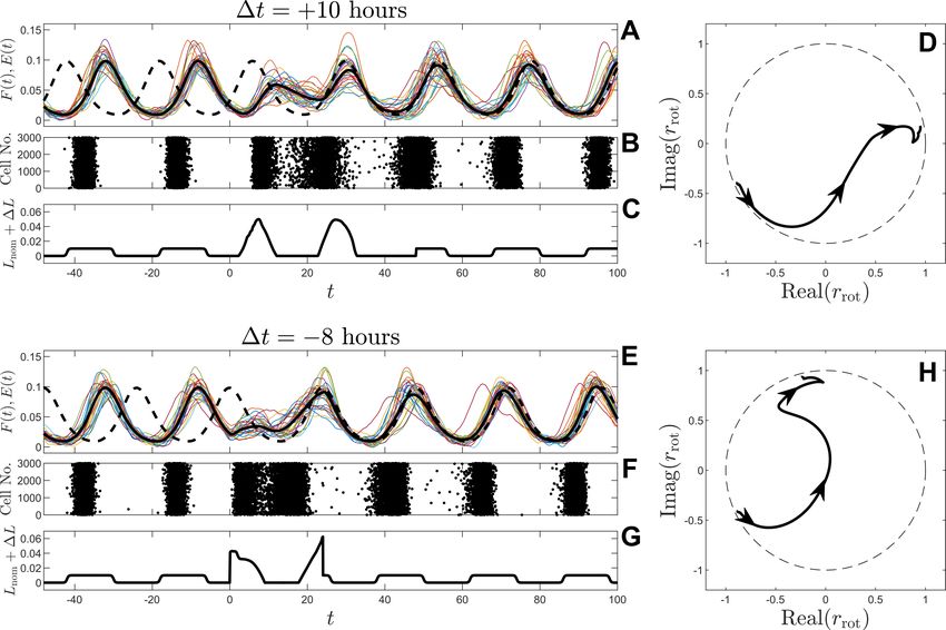
Letting Lc be the time-varying parameter used in the adaptive reduction (13), the traces of
B(θ) on the resulting periodic orbits xγLc are shown in panel A of Figure 1. The periodic orbits are
appropriately shifted so that θ = 0 corresponds to the moment that B(θ) reaches its peak value.
For all values of Lc considered, the periodic orbit has only one non-negligible Floquet exponent (the
other Floquet exponent is negative and large in magnitude). Along with this Floquet exponent,
the nominal period is shown as a function of Lc in panel B. The resulting phase and isostable
response curves for various values of Lc are computed using an adjoint method described in [55]
and shown in panels C and D, respectively. Finally, D and Q are computed according to (9) and
shown in panels E and F, respectively.
Figure 1: Traces of B γ (θ) are shown for (28) using various constant values of Lc . The resulting
natural frequencies and Floquet exponents are shown in panel B. The dashed line at κ = 0 is shown
for reference, emphasizing that all considered orbits are stable. Phase and isostable response curves
used in the adaptive reduction are shown in panels C and D, respectively. The terms D and Q
characterize how changing the nominal parameter influences the phase and isostable coordinate
and are shown in panels E and F, respectively. Note that both the magnitude of oscillations as well
as the magnitude of the Floquet exponents become smaller as Lc increases resulting less robust
oscillations.
For the moment, the optimal control problem will be considered taking L0 = 0. Additionally,
it will be assumed that Lmax = +∞, and Lmin = −∞. This situation represents a situation where
no entraining stimulus is applied and no bounds on the magnitude of light are present. While this
situation is not realistic, it provides insight into the limitations of each optimal control formulation.
10Note that when L0 = 0, the system is technically not entrained to any external stimulus. Never-
theless, the optimal control frameworks proposed in Section 3 can still be implemented by defining
xγent ≡ xγp0 with xγp0 |θ=0 = xγent |t=0 .
For various choices of ∆t, an optimal control is computed using the adaptive reduction frame-
work (with Equations (14), (19) and (20)), the first order accurate phase-amplitude reduction
strategy (with Equations (21) and (24)), and the phase-only reduction strategy (with Equation
(27)). For the phase-amplitude and phase-only reduction strategies, Lc is taken to be 0. The
constant β (which sets the penalty for large isostable coordinates) is taken to be 10−4 for the
phase-amplitude control strategy. Tf is taken to be 24 hours for all control strategies. Optimal
inputs ∆L(t) are computed using each reduction strategy, with the resulting inputs applied to the
full model (28).
Figure 2: Optimal control results when no external entraining stimulus is applied and no con-
straints are placed on ∆L(t). The resulting optimal controls computed using the adaptive reduction,
phase-isostable reduction, and the phase-only reduction are applied to the full model equations (28).
The specified ∆t is plotted against the resulting time change, ∆tact in Panel A. The error, defined
to be ∆tact − ∆t is shown in panel B. Specific inputs are shown for ∆t = +9 and -9 hours in panels
C and D using the specified method. Resulting traces of B(t) when these inputs are applied to
the full model are shown in Panels E and F, respectively. The black dashed line shows the fully
entrained solution after the time shift is applied. While all methods perform reasonably well for
for |∆t| < 3 hours, the phase-isostable and phase-only optimal control strategies that yield inputs
that give unexpected and inaccurate results. Conversely, the adaptive reduction strategy accurately
modifies the phase of the oscillation for any prescribed ∆t.
Resulting time shifts are shown in panel A of Figure 2. Note that because there is no external
entraining stimulus in this example, mandating a time shift ∆t is equivalent to mandating a phase
shift ∆θ = 2π∆t/24.2, and tact is the actual resulting phase shift when the input is applied to
the full model (28). ∆tact is computed by considering the infinite-time behavior after the input is
applied. In panel B, Error = ∆tact − ∆t is shown. For small values of ∆t, all reduction frameworks
produce stimuli that achieve the control objective. As the required ∆t shift increases, errors tend to
increase for the phase-only and the phase-amplitude control strategies. By contrast, the adaptive
reduction strategy yields results that are nearly perfect, with the maximum value of |∆tact − ∆t|
being less than 0.4 hours for any choice of ∆t. Panel C (resp., D) show resulting control inputs
11for each strategy that result when ∆t = +9 hours (resp. -9 hours). Panels panel E and F show
corresponding traces of B(t) that result when those inputs are applied to the full model (28).
Next, a situation where L0 = 0.01 is considered next so that the limit cycle is nominally
entrained to a the external 24-hour light-dark cycle (29). Noting that the nominal phase response
curves from panel C of Figure 1 can take values that are on the order of approximately 20, this
input is quite large for this system. Such situations have traditionally been difficult to approach
with standard phase reduction techniques (as discussed in [11]) because the entraining input is
often strong enough to drive the state far from its unperturbed limit cycle, thereby invalidating the
assumptions of the phase reduction. Alternative techniques that consider the dynamics of Poincaré
maps [11], [12] or those that consider the entrained orbit itself to be the nominal periodic orbit
[56] have been useful in some situations. As shown in the results to follow, the control strategy
that uses adaptive phase-amplitude reduction yields accurate results while the phase-only and first
order accurate phase-amplitude reduction strategies fail.
For this example, Lmin = 0 is chosen in optimal control problem along with Lmax = +∞ to
mandate Lnom +∆L ≥ 0 and reflect the constraint that negative light cannot be applied. Once again,
for various choices of ∆t, an optimal control is computed using the adaptive reduction framework
(from Equations (14), (19) and (20)), the first order accurate phase-amplitude reduction strategy
(from Equations (21) and (24)), and the phase-only reduction strategy (from Equation (27)). For
the phase-only reduction strategy β is set to zero, since the nominal 24-hour light-dark cycle makes
it difficult to limit the magnitude of the isostable coordinate. In all optimal control computations,
t0 = 0 which corresponds to the middle of subjective night. Tf is taken to be 24 hours for the
phase-only and adaptive reduction strategies. Tf is taken to be 72 hours for for the phase-amplitude
reduction strategy, it is not possible to find numerical solutions to the optimal control problem for
smaller values of Tf . Resulting inputs are then applied to the full model equations (28) with results
shown in Figure 3. Because the model is entrained to Lnom (t) in the absence of additional input,
the resulting recovery time, defined to be the time it takes for the phase to return to and stay
within one hour if its steady state behavior, is shown in Panel A. Results are also compared to the
nominal, uncontrolled recovery time (i.e. taking ∆L = 0). Note that the phase is only measured
at θ = 0, which can be observed once per cycle when B(t) reaches a local maximum. The recovery
time is inferred by computing the difference in time between the moment θ reaches 0 for the fully
entrained reference and the reentraining simulation and interpolating the time difference for all
values in between. If the time difference is less than one hour the first moment θ = 0 is reached
after input is applied for the reentraining system, the recovery time is taken to be equal to Tf .
The optimal controls computed according to the phase-isostable and the phase-only reduction
strategies generally have only a small influence on the recovery times and even occasionally result in
worse outcomes than if no input was applied at all. Conversely, the when the control identified when
using the adaptive phase-amplitude reduction is applied to the full model equations, the recovery
time exactly 24 hours indicating the system is recovered by the time the first measurement of θ = 0
is made after the optimal stimulus is applied. Panel B of Figure 3 shows Lc when the optimal
control is applied to the adaptive reduction. Panels C and D (resp., E and F) show the optimal
control inputs and traces of B(t) for a time shift of ∆t = +12 hours (resp. -8 hours). Black lines
also show traces of B(t) and the nominal light-dark cycle input during the uncontrolled recovery.
12Figure 3: Optimal Control results with a nominal external entraining stimulus and constraints on
the applied stimulus are considered. Panel A shows recovery times when applying the resulting
optimal inputs determined from each of the three optimal control formulations to the full model
equations (28). The uncontrolled recovery times are also showed for reference. The formulation
with the adaptive reduction significantly outperforms the other two control formulations. Indeed,
the phase-only and first order accurate phase-isostable formulations often yield control inputs that
increase the recovery time. Panel B shows the value of p, i.e., the parameter that corresponds to
the nominal periodic orbit during the application of the optimal stimulus for various time shifts ∆t.
Notice that p increases to much larger values for all but the smallest magnitude choices of ∆t. These
changes in p represent large deviations from the nominal limit cycle which has p0 = 0. The adaptive
reduction has the ability to explicitly incorporate these shifts, however, the phase-amplitude and
phase-isostable reductions cannot explicitly account for these shifts. This fundamental difference
between the reduction frameworks leads to the difference in efficacy between the resulting optimal
inputs. Panels C and D show the recovery for the optimal controls identified by each of the optimal
control formulations for ∆t = +12 hours. The black curve also shows the nominal recovery when
∆L(t) = 0. The dashed line in panel C represents the limit cycle that is fully entrained to the
shifted nominal input Lnom (t + ∆t). Panels E and F show the same information for a time shift of
-8 hours.
5 Control of Population-Level Oscillations and Data-Driven In-
ference of Reduced Equations
Here, a model for the behavior of a population coupled circadian oscillators will be considered:
K1n Bi KF
Ḃi = v1 − v2 + hc + αi (Lc + Lnom (ts ) + ∆L(t)),
K1n
+ Din K2 + Bi Kc + KF
Ci
Ċi = k3 Bi − v4 ,
K4 + Ci
Di
Ḋi = k5 Ci − v6 ,
K 6 + Di
Ei
Ėi = k7 Bi − v8 , i = 1, . . . , N. (30)
K8 + Ei
13The above model considers a population of N = 3000 coupled oscillators of the same form as (28)
with the addition of the dynamics of a neurotransmitter Ei that allows communication between
cells. Assuming that the spatial transmission of the neurotransmitter is fast relative P to the 24-
hour scale of oscillation, effective mean-field coupling is assumed with F ≡ (1/N ) N k=1 Ei , which
enters into the equation for the variable B. Additionally, in (30) each neuron has an intrinsic
sensitivity to light, αi , drawn from the distribution αi = max(1 + 0.4N (0, 1), 0) where N (0, 1)
is a normal distribution with zero mean and unit variance. Nominal parameters in this model
are taken to be n = 5, v1 = 0.868, v2 = 0.634, k3 = 0.7, v4 = 0.35, k5 = 0.7, v6 = 0.35, k7 =
0.35, v8 = 1, K1 = 1, K2 = 1, K4 = 1, K6 = 1, K8 = 1, hc = 1, Kc = 1, and K = 0.5. In order to
incorporate heterogeneity in the model, the parameters k3 , k5 , k7 , v4 , v6 , and v8 are drawn from a
normal distribution with the mean being the nominal parameter value and a standard deviation
equal to 0.01. In all simulations, independent and identically distributed zero mean white noise
with intensity 0.0002 is added to the variable Bi for each oscillator. Like in the single oscillator
equations (28), the external light-dark cycle Lnom (ts ) in (30) takes the form (29).
While each of the necessary terms of the reduction in (13) could be computed numerically, a
strategy for inferring the required terms from output data will be considered here, as would be the
case for an experimental system. The control strategy from Section 3 will then be applied to the
resulting adaptive reduction.
5.1 Data-Driven Methods for Computation of Terms of the Adaptive Reduction
When the underlying dynamical equations are known, it is relatively straightforward to compute the
necessary terms of the adaptive reduction (13) using the ‘adjoint method’ [6] and related equations
from [57] as described in Section 2. However, when the the dynamical equations are unknown,
the terms of the adaptive reduction must inferred from data. The ‘direct method’ [21], [38] is a
well-established technique for identifying the phase response curve from (4). Previous work [56]
developed a data-driven technique for computing the terms of the phase-amplitude reduction from
(5). This strategy will be expanded here to compute the necessary terms of the adaptive reduction
from (13). Here, it is assumed that the input also the sole time-varying parameter. While (13) has
only one isostable coordinate, this technique is relatively straightforward to extend to situations
where multiple isostable coordinates are involved.
For concreteness, the model (30) will be used assuming light perturbations ∆L(t) can be given
and that the single output F (t) (i.e., the mean value of Ei for the population) can be measured.
For the given parameter set it will be assumed that Equation (30) has only one dominant isostable
coordinate. Additionally, Lc will be taken as the time-varying paramater. In this situation, it is
possible to write the equations for the adaptive phase-amplitude reduced model in the form (13).
The terms of the adaptive reduction will be inferred using the procedure detailed below.
Step 1: With a static choice of Lc , and taking Lnom (ts ) + ∆L(t) = 0 for all time, the procedure
introduced in [56] can be used to identify ω(Lc ), κ(Lc ). This strategy can also be used to identify
ψ(t1 ) and θ(t1 ) provided θ(t1 ) ≈ 0 using a delayed embedding of the output from F (t1 ) to F (t1 +T ).
This strategy is summarized in Figure 4. To apply this strategy, the model is first simulated until
transient behaviors have died out. A threshold is chosen to denote θ ≈ 0 (in this case, θ ≈ 0
corresponds to the moment F (t) crosses 0.045 with a positive slope). Over multiple oscillations,
the average period at which this threshold is crossed is taken to be the period of oscillation, T . A
set of delay embeddings, each which start the moment that F (t) crosses 0.045 and end T hours
later, is recorded and the average value of the output F over these measurements is used as an
approximation for the stable periodic orbit F γ (t) as shown in panel B of Figure 4. Once the periodic
14orbit is obtained, the recovery to the periodic orbit from a perturbed initial condition is considered
in order to determine the isostable coordinates. As shown in panel A, the coupling strength K is
decreased 50 percent for t ∈ [0, 200] hours. For t > 200, K is set back to its nominal value, and a
series of delayed embeddings from tj to tj + T are taken, where each tj is chosen so correspond to
a moment that F (tj ) crosses 0.045 with a positive slope. This procedure is repeated over multiple
trials. The periodic orbit is subtracted from the resulting embeddings with individual traces shown
in panel C. To proceed, let yj ∈ Rq correspond to the j th delay embedding from panel C. In other
words, yj is comprised of the output from tj to tj + T after F γ is subtracted. Here, q = (T /δt) + 1
where δt is the sampling rate.
Figure 4: A data-driven strategy for identifying phase and isostable coordinates from the large
circadian model (30). In panel A, the model is perturbed from its limit cycle by decreasing K by
a factor of 2 for 200 hours (red curve). The subsequent recovery takes approximately 400 hours
(blue curve) and the black curve represents the behavior once the model has recovered to the
stable limit cycle. As shown in panel B, the periodic orbit F γ (t) (black line) is taken to be the
average of multiple cycles once transient behavior has died out. Using data obtained from the blue
portion of panel A, multiple delayed embeddings are obtained and shown in panel C that represent
the deviation from the periodic orbit on a particular cycle. POD is performed on the data from
panel C and identifies two characteristic modes. The POD modes are transformed to represent the
deviation from the periodic orbit in a basis of phase and isostable coordinates with modes shown
in panel E. As described in the text, this procedure allows one to measure the isostable coordinates
at specific times, and a the slope of the linear regression shown in Panel F represents the Floquet
multiplier corresponding to the isostable coordinate.
Proper orthogonal decomposition (POD) [4], [19], [51] is applied to the data shown in panel C
in order to identify a small number of representative modes. In this case, 2 modes are sufficient
to represent the data from panel C, denoted by φ1 ∈ R q q
and φ2 ∈ R and shown in panel D as
blue and red curves, respectively. The transformation µ1 µ2 = φ1 φ2 A where A is a 2 × 2
†
nonsingular square matrix and is chosen so that µ1 = φ1 φ2 g γ where g γ ∈ Rq corresponds to
dF γ /dt taken at the sampling rate δt and † represents the Moore-Penrose pseudoinverse. Plots of
µ1 and µ2 are shown in panel E in blue and red, and are proportional to the shifts in the output
resulting from a shift in θ and ψ, respectively. Furthermore as described in [56], the vectors η1
T T
and η2 defined according to, A−1 φ1 φ2 = η1 η2 can be used to compute the phase and
15isostable coordinates at specific instances in time according to the relationships
cη1T yj = θ(tj ),
η2T yj = ψ(tj ), (31)
where c is a constant that can be determined using a strategy discussed in [56]. This information
can be used to track ψ over successive periods during the recovery as plotted in panel F. The slope
of a linear regression of this data gives an approximation of the Floquet multiplier, Λ, corresponding
to ψ and the Floquet exponent can be computed according to the relationship κ = log(Λ)/T .
Note that the procedure from Step 1 represents an implementation of the procedure given in
Section IV,A from [56] for a constant choice of Lc . The interested reader is referred to [56] for a
more detailed description of this method. This strategy is repeated to determine the associated
terms of the phase and isostable coordinate reduction for various values of Lc .
Step 2: For a given choice of Lc the terms of z and i can be inferred directly by applying a series
of pulse inputs and measuring the resulting change in the phase and isostable coordinates. This
can be accomplished with a strategy akin to the direct method [21], [38] whereby a pulse input of
magnitude dL is applied for a short duration of time as shown in panel B of Figure 5. Complete
cycles of the output starting at θ ≈ 0 (corresponding to a positive crossing F (t) = 0.045 threshold)
beginning at t1 and t2 preceding and following the input can be extracted as shown in panel A, and
the relationships from (31) can be used to determine θ(t1 ), θ(t2 ), ψ(t1 ), and ψ(t2 ). Assuming the
pulse input was applied at t = 0, the shift in phase can be computed by recalling that the phase
would have simply increased at the rate ω had the input not been applied. The deviation, ∆θ,
from this expectation can be assumed to be the change in phase caused by the input. Likewise, by
assuming that ψ decays exponentially towards zero at a rate governed by κ in the absence of input,
ψ can be computed immediately before and after the applied input to infer the change in isostable
∆θ ∆ψ
coordinate ∆ψ. For the chosen parameter Lc , z(θ, Lc ) ≈ dLdt and i(θ, Lc ) ≈ dLdt , where dt is the
duration of the perturbation applied at phase θ. This process can be repeated for multiple trials
to obtain approximations of i(θ, Lc ) and z(θ, Lc ) as shown in Panels C and D of Figure 5 and the
resulting data can be fit using an appropriate basis.
Step 3: Both D and Q can be inferred using a strategy similar to the one described in Step 2. In
this case, instead of a brief pulse, the total applied light is shifted from Lc to Lc + dL at a known
time as shown in panel F of Figure 5. This shift can be viewed as a sudden change in the nominal
parameter by dL centered at Lc + dL/2; in other words a pulse to L̇c of magnitude dL. Considering
the structure of the reduced Equations (13), this pulse in L̇c can be used to infer both D and Q in
a manner similar to the direct method for identifying z and i. Similar to the procedure used in step
2, cycles beginning at t1 and t2 preceding and following the step function change in input as shown
in panel E of Figure 5 can be isolated from the output. Subsequently, Equations (31) can be used
to identify θ(t1 ), θ(t2 ), ψ(t1 ), and ψ(t2 ). Note that for each trial θ(t1 ) and ψ(t1 ) (resp. θ(t2 ) and
ψ(t2 )) must be found using η1 and η2 that are obtained from Step 1 taking the nominal parameter
to be Lc (resp. Lc + dL). Using the same reasoning employed as part of Step 2, the change in
phase, ∆θ, and isostable coordinate, ∆ψ, caused by the parameter change can be inferred yielding
individual data points for D(θ, Lc + dL/2) = ∆θ/∆p and Q(θ, Lc + dL/2) = ∆ψ/∆p. This process
can be repeated to obtain multiple data points; curves can be fit to the resulting data as shown in
panels G and H of Figure 5.
Step 4: Steps 3 and 4 can be repeated for various choices of Lc to obtain a series of curves used
in the reduced equations of the form (13). Resulting information obtained when applying the
procedure from Steps 1 through 4 to the model from (30) are shown Figure 6. Numerical trials
16Figure 5: Inferring the phase and isostable response to pulse and step function inputs to infer the
terms of the reduction (13). For a nominal value of Lc , a short pulse can be applied as in panel
B. Data from a complete cycle occurring both before and after the perturbation (red curves in
panel A) are used to identify the phase and isostable coordinates at t1 and t2 . This information is
then used to obtain a discrete measurement of z(θ, Lc ) and i(θ, Lc ), and this process is repeated
multiple times. Each trial yielding a single measurement of both z and i which are represented
by black
P dots in panels C and D. The blue lines are obtained by fitting the sinusoidal basis of the
form 3n=0 [an sin(nθ) + bn cos(nθ)]; the resulting fits are taken to be the response curves. Likewise,
panels E through H illustrate a similar procedure for obtaining D and Q. Instead of applying pulses,
step function inputs are applied (panel F), complete cycles before and after the step function are
extracted (panel E) and used to infer the change in phase and isostable coordinates resulting from
the input. Each trial gives a single data point for D and Q (black dots in panels G and H). This
process is repeated for multiple trials and the same sinusoidal basis is used to fit the data (blue
lines).
are performed taking Lc ∈ {−0.01, 0.01, 0.03, 0.05, 0.07}, and all other curves are obtained through
interpolation.
17Figure 6: Resulting terms of the adaptive reduction (13) resulting from the data-driven inference
strategy from Section (5.1). For all limit cycles, θ = 0 corresponds to the moment that F (t) crosses
0.045 with a positive slope. As Lc increases, the magnitude of the nominal oscillations decrease as
shown in panel A. Panels B and C give the natural frequency and Floquet exponent as a function
of Lc . Panels D-F show specific terms of the adaptive reduction for various values of Lc .
5.2 Optimal Control of Oscillation Timing Results
The terms of the adaptive reduction inferred using the strategy from Section 5.1 and shown in
Figure 6 are used to implement the optimal control strategy for manipulating oscillation timing as
described in Section 3. The nominal value of Lc is taken to be zero and the nominal magnitude of
the light-dark cycle is taken to be L0 = 0.01. Bounds on the total allowable light input are chosen
to be Lmin = 0 and Lmax = ∞ so that negative light inputs are not possible. Recalling that the
choice of ∆t in the control formulation corresponds to a sudden change in the environmental time
(perhaps due to rapid travel across multiple time zones) the optimal control input is computed for
various choices of ∆t with the adaptive reduction framework (from Equations (14), (19) and (20))
and the first order accurate phase-amplitude reduction strategy (from Equations (21) and (24)).
For when using the first order phase-amplitude reduction strategy, β is set to zero since the nominal
24-hour light-dark cycle makes it difficult to limit the isostable coordinates. For many choices of ∆t,
the phase-only optimal control equations (27) have solutions that grow to infinity in finite time;
consequently this optimal control formulation will not be considered for this application. In all
optimal control computations, t0 = 0 which corresponds to the middle of subjective night. When
possible, Tf is taken to be 24 hours. For positive time shifts and particularly large magnitude
negative time shifts, solutions of the optimal control equations were not able to be found using
Tf = 24 hours. In these cases, Tf is instead taken to be 48 hours.
The numerically determined optimal control inputs are applied to the full model equations (30)
with results shown in Figure 7. The recovery time in panel A is defined to be the time required
(after the time shift by ∆t of the light-dark cycle) for the phase to return to and stay within two
hours of its steady state behavior. The nominal recovery time that results when ∆L is zero is also
shown for reference. Note that the moment that F (t) crosses 0.045 is used to correspond to the
time that θ = 0 and that this can only be observed once per cycle – for this reason, if the phase is
18You can also read