Optimal Regional Labor Market Policies - IZA DP No. 14204 MARCH 2021 Philip Jung Philipp Korfmann Edgar Preugschat - Institute of ...
←
→
Page content transcription
If your browser does not render page correctly, please read the page content below
DISCUSSION PAPER SERIES

IZA DP No. 14204

Optimal Regional Labor Market Policies

Philip Jung
Philipp Korfmann
Edgar Preugschat

MARCH 2021
DISCUSSION PAPER SERIES

IZA DP No. 14204

Optimal Regional Labor Market Policies

Philip Jung
TU Dortmund and IZA
Philipp Korfmann
TU Dortmund
Edgar Preugschat
TU Dortmund

MARCH 2021

Any opinions expressed in this paper are those of the author(s) and not those of IZA. Research published in this series may
include views on policy, but IZA takes no institutional policy positions. The IZA research network is committed to the IZA
Guiding Principles of Research Integrity.
The IZA Institute of Labor Economics is an independent economic research institute that conducts research in labor economics
and offers evidence-based policy advice on labor market issues. Supported by the Deutsche Post Foundation, IZA runs the
world’s largest network of economists, whose research aims to provide answers to the global labor market challenges of our
time. Our key objective is to build bridges between academic research, policymakers and society.
IZA Discussion Papers often represent preliminary work and are circulated to encourage discussion. Citation of such a paper
should account for its provisional character. A revised version may be available directly from the author.

                                                     ISSN: 2365-9793

                                           IZA – Institute of Labor Economics
Schaumburg-Lippe-Straße 5–9                      Phone: +49-228-3894-0
53113 Bonn, Germany                             Email: publications@iza.org                                    www.iza.org
IZA DP No. 14204 MARCH 2021
ABSTRACT
Optimal Regional Labor Market Policies
We document large and persistent spatial dispersion in unemployment rates, vacancies,
labor market tightness, labor market flows, and wages for Germany on a granular regional
level. We show that in the 1990s differences in inflows from employment to unemployment
were the key driver of regional dispersion in unemployment rates while in the 2000s
outflows became more important. To account for the documented regional dispersion
we develop a spatial search and matching model with risk-averse agents, endogenous
separations and unobservable search effort that leads to moral hazard and quantify the
relative importance of 4 potential structural driving forces: dispersion in productivity,
in the bargaining strength of workers, in idiosyncratic risk components and in regional
matching efficiency. Based on region-specific estimates of these factors we then study the
resulting policy trade-off between insurance, regional redistribution and efficiency. We
design (optimal) region-specific labor market policies that can be implemented using hiring
subsidies, layoff taxes, unemployment insurance benefits and transfers financed by social
insurance contributions. We find that a move towards an optimal tax system that explicitly
conditions on regional characteristics could lead to sizable welfare and employment gains.
JEL Classification: J50
Keywords: optimal labor market policies, regional unemployment
Corresponding author:
Philip Jung
Faculty of Business, Economics and Social Sciences
Technical University of Dortmund
Vogelpothsweg 87
44227 Dortmund
Germany
E-mail: philip.jung@tu-dortmund.de1 Introduction
Regional earnings and unemployment disparities are large and persistent in Germany. East
German workers for example earned 30% less on average during the period 1994-2004 and
faced unemployment rates of 20%, twice as high as West German workers. These differences
are not a permanent fate though. A decade later, in 2014, the striking divide between the
East and the West is still visible in unemployment rates, but it became much less pronounced.
Unemployment rates have almost halved to 10% on average in the East and were only 60%
larger than in the West. However, the catch-up of the East masks substantial variation across
regions when looking at a more granular scale. Many employment districts in the West fell
behind and the gap between booming southern districts and the rest of the country has
widened over time.
In this paper we address three interdependent questions: are flows into or out of unem-
ployment the key drivers of regional dispersion in unemployment rates in Germany? What are
the underlying structural causes for regional dispersion in these flows? Is regional dispersion
inefficient and - if so - what region-specific instruments can be used to improve employment
and welfare?
We answer these questions by studying regional dispersion and its consequences for re-
gional policy based on German employment agency district data for the years 1994-2014.1
We empirically document spatial dispersion and time trends for key labor market variables
like in- and outflow rates, vacancies, market tightness, and wages utilizing administrative mi-
cro data and a newly digitized data series of job openings. We show that inflows have been
the key driver of regional unemployment dispersion for the nineties, as emphasized by Bilal
(2019) for France, but outflows dominate the picture after the so-called Hartz reforms of the
unemployment insurance system in 2005. To explain the cross-sectional dispersion and the
trends over time we develop a multi-region variant of a structural search and matching model
based on Jung and Kuester (2015) that includes risk-averse agents, endogenous separations
and unobservable search effort. The model features a trade-off between insurance, redistri-
bution and efficiency considerations and implies a rich set of region-specific instruments to
counteract frictions above and beyond the classical search externalities (Kline and Moretti,
2014). We use the model to estimate the relative importance of potential underlying causes
for regional dispersion that have been suggested in the literature: dispersion in productivity,
matching efficiency, bargaining strength and idiosyncratic firm risk. We then quantify the
relative importance of each of these channels in explaining regional dispersion for Germany.
Taking the estimated structural labor market differences as policy-invariant (at least in the
shorter run), we then use the model to ask how an optimal labor market policy could look
like in Germany. We offer a quantitative exploration of the regional-specific differences in
1
Part of the paper is based on a dissertation chapter of Korfmann (2020).
1key tax instruments necessary to decentralize a constrained efficient allocation and study the
resulting employment and welfare gains. We describe these steps and our findings in more
detail next.
We use data from the employment panel of integrated employment biographies (SIAB)
and monthly vacancy stocks obtained from the federal employment agency (BA) to ask
whether inflows into unemployment account for the bulk of the regional dispersions or whether
outflows from unemployment are more important in Germany.2 An examination of the evo-
lution of the underlying worker flows can help to discriminate between various potential
explanations for regional dispersion: In the decade 1994-2004 (before the German Hartz IV
reform) inflows into unemployment account for 70% of the regional dispersion in unemploy-
ment rates, in line with findings for France (Bilal, 2019). However, in the aftermath of the
Hartz reforms (see Hartung et al., 2018) the picture changes. Regional variation in inflows
rates have declined substantially, which coincides with a sharp decrease in the level of these
rates throughout all districts. At the same time differences in outflow rates across regions
have increased, while the average increase in outflow rates over time is small. In the decade
following the Hartz reforms (2005-2014) - largely driven by the booming southern states - out-
flows become substantially more important and account for 60% of the regional dispersion.3
A story to tell is a tale of two regions: East Germany and North Rhine-Westphalia (NRW),
the former coal area and most densely populated region in the Western part of Germany.
Districts located in these two regions exhibited the highest unemployment rates already in
1994 but due to different reasons. In NRW, unemployment was high because outflow rates
were low, while East German districts exhibited above-average inflow rates. Throughout our
observation period, unemployment rates in East Germany approached West German levels
and this catch up was driven by a substantial decrease in inflow rates. Districts in NRW,
however, fell behind as outflow rates did not rise, as they did in the southern districts, and
the declines in inflows were the lowest in the country.
Can the above stylized facts inform us about structural differences across regions? To
answer this question we develop a multi-region variant of a structural search and matching
model based on Jung and Kuester (2015) that features immobile risk-averse agents, endoge-
nous separation and moral hazard leading to a trade-off between regional insurance, redistri-
bution and efficiency. We treat a district as a closed labor market by assuming away labor
2
Our research is related to the literature on the ins and outs of labor markets flows (e.g. Elsby et al.,
2011). Although differences in regional unemployment rates in Germany are well documented (Patuelli et al.,
2012), an analysis of the underlying labor market flows is still missing from the literature.
3
The new evidence we provide on the importance of inflows vs. outflows rates for unemployment differ-
entials echoes findings of the research on the importance of worker flows for the development of the aggregate
unemployment rate in Germany, see Hertweck and Sigrist (2015), Jung and Kuhn (2014), Hartung et al.
(2018) for Germany. Concerning other countries, our results for the nineties are in line with those of Bilal
(2019), who finds that inflows explain the majority of the variations in regional unemployment rates in the
U.S. and France. We add that the explanatory power of inflow rates is time-varying.
2mobility across these markets.4 We estimate the model with a uniform tax and unemploy-
ment insurance (UI) benefit system on the federal level that capture stylized aspects of the
German system. The purpose of the model is twofold: First, we use the model to estimate
regional differences in key parameters that might capture underlying structural differences
across regions. Second, given these estimates on regional heterogeneity, we ask how a policy
maker could design a tax and transfer scheme that optimally addresses regional disparities.
To this end we allow regions to differ along 4 dimensions that have been suggested in the
literature to account for regional dispersions over space: (1) A wage channel capturing the
idea that East German wages had been set ’too high’ relative to productivity after reunifica-
tion forcing workers into unemployment or migration to the West (Burda and Hunt, 2001),
which gives wage setting by (Western) unions a key role in explaining regional dispersions;
(2) A matching efficiency channel that allows for regional differences in matching particular
skill requirement of jobs to unemployed workers (Fahr and Sunde, 2006); (3) A productivity
channel, that - due to sorting decisions by firms or agglomeration forces (Bilal, 2019) - lead
to regional differences in labor market outcomes; (4) An idiosyncratic risk channel in which
differences in firm characteristics across space (Eeckhout et al., 2014) translate into larger
idiosyncratic uncertainty of the profit path of a given match. We look at regional data aver-
aged over two time periods, 1994-2005 and 2006-2014, before and after the Hartz reforms and
back out the respective structural parameters sets based on a steady state approximation of
the model in both periods. We allow the benefit system to change over time to potentially
capture a fundamental break in German labor market institutions due to the Hartz 4 reforms
that has affected in particular the inflow rates over time as shown in Hartung et al. (2018).5
The model allows us to quantify the relative importance of these channels based on regional
variations in wages, in- and outflows and market tightness.
When viewed through the lens of a search and matching model the large differences in
wages during the nineties need to be explained by large differences in productivity in the
East. Over time however, a catch-up process has let to a relative increase in productivity
in the eastern districts by over 20%. Productivity increases (at least relative to vacancy
creation cost) would tend to increase outflow rates in most models that follow Mortensen
and Pissarides (1994). However, the probability of finding a job has barely changed between
1994 and 2014 in the East. To account for these facts wage setting is a key driver in the
East. To rationalize observed outflow rates the model demands a strong bargaining position
of workers in the East during the nineties pushing wages up relative to productivity compared
4
Inter-regional migration in Germany is not negligible, but as we show in a companion paper (Jung et
al., 2021) it is limited and heavily concentrated in young age cohorts. We provide an upper bound on the
gains from mobility using the mismatch index developed by Sahin et al. (2014), see appendix (D.0.1).
5
The literature investigating the Hartz reforms is extensive. See, for example, Hertweck and Sigrist
(2015), Launov and Wälde (2016), Klinger and Rothe (2012), Krause and Uhlig (2012), Klinger and Weber
(2016).
3to other western regions in line with some narratives pointing towards unions from the West
that aimed at keeping East German wages close to western standards (see Burda and Hunt,
2001). Over time, however, the bargaining strength of unions declined. Tightness data and
outflow rates together identify the underlying matching efficiency by region. Interestingly,
we find that in the nineties the East and the South, home to the districts with the lowest and
the highest productivity, face similar high levels of matching efficiency. The West and the
North, in contrast, were less efficient in matching worker to firms. Over time, the matching
efficiency in the East declined somewhat, but remained through out the 2000s larger than in
the North or the West. Finally, to explain the regional dispersion in inflow rates we find that
idiosyncratic productivity risk is a bit higher both in the former coal area in NRW as well as
in the East. The Hartz reforms lead to an increase in the match surplus in all districts that
has lowered inflow rates substantially.
The estimated structural disparities might call for region-specific policies (Glaeser and
Gottlieb, 2008 and Kline and Moretti, 2013).6 The design of these policies will depend
crucially on the determinants of local unemployment and possible underlying inefficiencies:
for example, a measure designed to increase hirings in eastern Germany might not be well
suited when unemployment is high because employment relationships are terminated more
often. Once we have an estimate on regional differences in primitive parameters in place
we can ask how an optimal regional labor market policy mix would look like. With the
optimal policy mix, the planner implements the constrained-efficient allocation, given the
unobservable search effort of workers. Our model provides simple formulas for the design of
optimal hiring subsidies in a region, optimal firing taxes as well as optimal net replacement
rates of the UI benefit system both for a world without redistribution across regions, i.e.
in a setup where we require the tax-code to be self-financing within a region, and with
redistribution, where we allow for transfers across districts. We find only a small role for
variations of the unemployment insurance replacement rate by region, being lowest in the East
and in the South reflecting relatively high matching efficiency levels. The planner’s optimal
hiring subsidies and layoff taxes, however, vary substantially across districts, though in a way
that again comes at a surprise if one only looks at heterogeneity across unemployment rates.
In both periods, East German districts are subject to policies at a rather average level, while
the layoff taxes and hiring subsidies are particularly high in NRW and lowest in Bavaria. The
6
While Kline and Moretti (2013) abstract from the layoff margin and studies the relations ship between
outflows and hirings subsidies based on deviations of the Hosios condition, there is little work that accounts
for the importance of both layoffs and hirings. The present article is closest to the study of Bilal (2019), who
rationalizes regional variations in job losses and hirings in a model with worker and firm mobility. In his
model, spatial unemployment rate differentials are due to pooling externalities that drive the location choice
of firms: High productive firms co-locate in slack labor markets, while low productive firms locate in tight
labor markets. The co-location of the latter leads to high unemployment that is driven by high separation
rates in tight labor markets. Our empirical results point to a more complex mechanism, as we do not observe
that higher layoff rates coincide with tighter labor markets.
4social planner would subsidize job openings in NRW by twice as much as in the South and
by around 30% more compared to the East. Moreover, it would prevent separations by large
firing taxes also twice as high relative to average wages as in the South. This result is due to
the estimated large idiosyncratic risk component that explains the NRW data. The optimal
labor market policy mix leads - in the absence of any redistribution across districts - to gains
in employment of around 2% in the South and up to 8% in the East during the 2000s, in
the nineties potential employment gains were even larger. The corresponding welfare gains
are more homogenous across regions and sizable (around 23%). These gains are achieved by
ensuring that worker and firms, when making hiring and firing decisions, internalize the cost
and gains on the social inurance system properly. If one were willing to impose a utalitarian
planner and would allow for regional transfers an optimal policy would then equalize average
consumption across regional districts which implies substantial transfers to the East but
would not equalize employment opportunities. In fact the optimal policy mix with respect
to labor market institutions would hardly change.
This paper is organized as follows. Section 2 describes the data, discusses the sample
selection and provides a detailed overview on the development of local labor markets in
Germany. In section 3, we present the model. Section 4 estimates the model, relates regional
variations to structural model parameters and quantitatively evaluates the optimal policy
mix. Section 5 concludes.
2 Regional labor market development
This section briefly introduces the microdata we utilize to construct local unemployment rates
and workers flows. More details are provided in appendix A. We then provide a comprehensive
overview of the development of regional labor markets in Germany.
2.1 Data and sample selection
Our primary data source is the employment panel of integrated employment biographies
(SIAB), an administrative data set provided by the Institute for Employment Research
(IAB).7 The SIAB is a two-percent representative sample of all individuals who are un-
employed or subject to social insurance contributions and covers the years 1975 − 2014. The
panel represents approximately 80% of the labor force, as self-employed and civil servants
are excluded. We focus our analysis on the period 1994 − 2014 to include East German
7
This study uses the weakly anonymized version of the SIABSample of Integrated Labour Market Bi-
ographies (Years 1975 - 2014). Data access was provided via on-site use at the Research Data Centre (FDZ)
of the German Federal Employment Agency (BA) at the Institute for Employment Research (IAB) and
subsequently remote data access.
5workers, but occasionally report results for West-Germany for the years 1980-1994.8 . The
individual employment histories are used to construct monthly unemployment, inflow rates,
and outflow rates. This data is merged with monthly vacancy data. We obtain data on the
vacancy stock for 2000 − 2014 from the federal employment agency and combine them with
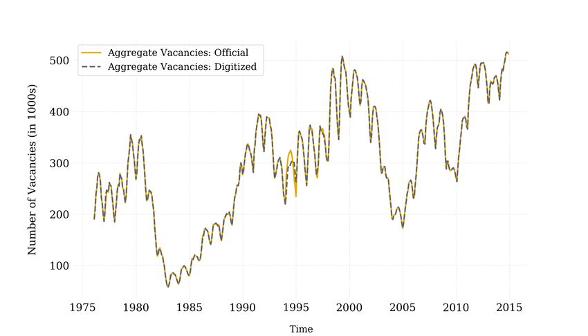
newly digitized data from their official historical reports. The construction of monthly worker
histories follows Jung and Kuhn (2014). In particular, we aggregate the daily employment
histories to a monthly frequency using predefined reference weeks. Labor market states are
assigned to a worker based on a hierarchical ordering, see appendix A for the details.
The regional level of analysis is the employment agency district. The territory of each
EAD is based on the geographical division of 2014. There are 154 districts. We treat the
three EADs covering Berlin as a single one because the territorial borders were subject to
many changes during the observation period. Each district includes approximately three
municipalities (Kreise, NUTS3). The SIAB data contains information on the municipality in
which the workplace is located for every employed worker. In contrast, information on the
place of residence for employed and unemployed workers is only available from 1999 onwards.
To obtain consistent data on regional transitions covering the whole observation period, we
assign the district of the last employment spell as the current place of residence when an
individual becomes unemployed. We impute the location information of unemployed workers
entering from non-employment by setting it to the location of their next employer if the
employment is consecutive.
We obtain data on registered vacancies from the federal employment agency for the years
2000 to 2014. Earlier data is digitized using the official monthly as well as annual reports
(Amtliche Nachrichten der Bundesagentur für Arbeit) of the employment agency. We observe
the number of vacancies that are reported to the FEA, which cover approximately 40 − 50%
of all vacancies (Brenzel et al. (2016)). However, other sources are not representative at this
highly disaggregated regional level. Moreover, the reported vacancies before 2000 include
job offers for seasonal workers or promoted vacancies, while the vacancies received from the
FEA are based on a modified concept, where seasonal jobs and promoted jobs are excluded.
We re-scale vacancies before 2000 by a constant factor to account for the level shift.9 The
geographical area corresponding to an EAD stayed roughly constant until the year 2012, after
which a significant reorganization of the territory took place. As the regional level of the SIAB
data is based on the division of territory in 2014, we adjust the vacancy data correspondingly.
Specifically, we use overlapping data for old and new territorial classifications to modify the
vacancy counts to be representative of the 2014 allocation of territory. The modifications of
the vacancy data are discussed in detail in appendix A.3. Overall, we assemble a regional
8
Information on workers in East Germany in 1992 and 1993 is used to impute the location variable.
9
We re-weight vacancies before 2000 by a factor of 0.7 to account for job offers for seasonal workers or
promoted vacancies. The adjustment factor is based on overlapping aggregate vacancy data from Hartmann
and Reimer (2010) for the period 2001 − 2009.
6data set spanning the years 1980−2014 for West and 1994−2014 for West and East Germany.
2.2 Regional labor market disparities
This section provides a comprehensive overview of the development of disparities in regional
labor markets over time. To better visualize the spatial variations, we group the unemploy-
ment agency districts according to their cardinal directions. However, to highlight the specific
labor market characteristics of the former coal and steel region situated in the federal state
North Rhine-Westphalia we subdivide the western districts into “NRW” and “South-West”
(or “S-W”) so that we obtain 5 main regions (see the map in Fig. 1).10
Figure 1: Map of employment agency districts and regions
Notes: The black grid lines indicate EAD borders, the colored regions indicate the five regions.
10
South: Bavaria and Baden-Wuerttemberg; NRW: North Rhine-Westphalia; South-West (S-W): Hesse,
Saarland, and Rhineland Palatinate (dark green); North: Schleswig-Holstein, Hamburg, Bremen, and Lower-
Saxony; East: Berlin, Saxony, Saxony-Anhalt, Thuringia, and Mecklenburg-West Pomerania. Note, we
summarize the regions South, South-West, West and North by “West Germany” and East we also call “East
Germany”.
7Figure 2 shows the development of unemployment rates during 1994-2014. In 1994,
eastern EADs were decoupled from the others as they exhibit unemployment rates almost
twice as high. While the average difference to West German EADs had declined up to
2004, unemployment had increased to even higher levels across all districts. During the
subsequent ten years, unemployment rates decreased significantly, but dispersion, measured
as squared deviation from the average started to increase around the year 2004 as documented
in appendix C.
Figure 2: Unemployment rates by employment agency district
Notes: The figure displays the average monthly unemployment rate in 154 employment agency districts for
the years 1994, 2004 and 2014.
The development also provides suggestive evidence about which districts are responsi-
ble for the increase in the dispersion of the unemployment rates in West Germany and the
stagnating dispersion in Germany. We find that it is predominantly districts located in
North-Rhine Westphalia that exhibit high unemployment rates in 2014, while eastern EADs
unemployment rates have almost converged to West German levels. Overall, while the dis-
persion across EADs increased, regional unemployment rates decreased by 54% on average,
from 1994 to 2014.
In the following paragraphs, we link the observed differences in unemployment rates to the
underlying variations in worker flows. As can be seen from Figure 3, the high unemployment
rates in East Germany are not the result of lower transitions out of unemployment. The
outflow rates are similar across all but the southern EADs, where we observe approximately
50% above-average rates for all points in time. The rates are stable over the observation
period. In fact, the average change between 1994 and 2014 was 5.0%. This small change
indicates that outflow rates are not the major driver of the between-district or over-time
variation in unemployment rates. The distribution of inflow rates, which is shown in Figure 4,
paints a different picture of regional disparities. Foremost, it is remarkably similar to the
distribution of unemployment rates: Inflow rates in East German districts are more than
8Figure 3: Outflow rates by employment agency district
Notes: The figure displays the average monthly unemployment inflow rate in 154 employment agency districts
for the years 1994, 2004 and 2014.
twice as high in 1994 and 2004, compared to all other regions. In 2014, the differences had
almost completely vanished, which is reminiscent of the low dispersion. Overall, we observe
an average decrease in the inflow rates of 63% throughout the sample period.
Figure 4: Inflow rates by employment agency district
Notes: The figure displays the average monthly unemployment inflow rate in 154 employment agency districts
for the years 1994, 2004 and 2014.
Unemployment rate decomposition We employ a two-state stock-flow model to quan-
tify the importance of the transitions in and out of unemployment for the variation in unem-
ployment rates across districts. Specifically, we exploit the steady state relationship of the
unemployment rate where u∗j = ξjξ+f jt
j
approximately holds (Fujita and Ramey, 2009). We
decompose the volatility around the average unemployment rate in each year
¯ − (1 − ū) ln(fj /f¯) + j ,
ln(u∗j /ū) = (1 − ū) ln(ξj /ξ) (1)
9where a bar denotes the average rate across districts and denotes the error term. We write
this expression in abbreviated form as du = dξ + df + . Fujita and Ramey (2009) show that
ln(uj /ū) can be decomposed into
Cov(du, dξ) Cov(du, df ) Cov(du, )
1= + + , (2)
V ar(du) V ar(du) V ar(du)
where, e.g., Cov(du,dξ)
V ar(du)
measures the contribution of the inflow rate to the variation of the
unemployment rate across districts. Table 1 presents the results.11
They mirror the observed changes of the distribution of outflow and inflow rates, as
displayed in Figures 3 and 4. Over the sample period, inflow rates account for, on average,
59% of the unemployment rate variation across EADs. However, their contribution decreases
from 70% in 1994-2004 to 43% in 2005-2014. Variations in outflow rates account for, on
average, 42% and their importance increases from 31 in 1994-2004 to 58% in 2005-2014.
Table 1: Decomposition of regional unemployment rate disparities
1994 - 2014 1994 - 2004 2005 - 2014
Outflows 0.42 0.31 0.58
Inflows 0.59 0.70 0.43
Notes: The table presents the results of a variance decomposition of the unemployment rates across districts
for different time intervals. “Outflow” (“Inflow”) indicates the contribution of the rate to the variation of
unemployment rates across districts.
Our descriptive evidence shows that differences in inflow rates are the main reason for
the variation in unemployment rates during 1994-2004. Bilal (2019) also finds that variations
in job losses explain a significant part of regional unemployment rate differentials in the U.S.
and France. However, inflow rates have become much more similar across EADs after the
Hartz reforms, while the differences in outflow rates have increased. As a result, the latter
have become more critical in the determination of regional differences in unemployment rates.
Wages and vacancies Figure 5 displays the deviations of the wage from the average wage
across districts in each year. Wages exhibit a substantial dispersion across EADs and this
dispersion is very persistent as the correlation between 1994 and 2014 is above 0.9. They are
lowest in East German EADs. However, eastern districts catch up to the average wage as
the gap is reduced from −30% in 1994 to −20% in 2014.
While unemployment rates are one of the most important labor market indicators, labor
market tightness is also informative with respect to the state of the economy. Figure 6 displays
11
Note, in the table and in the following we have ignored the contribution Cov(du, )/V ar(du), which is
negative but very small. Therefore, the contributions of the main components do not sum exactly to 100%.
10Figure 5: Wages by employment agency district
Notes: The figure displays the average (log) deviation of the wage from the average wage in each year in 154
employment agency districts for the years 1994, 2004 and 2014.
labor market tightness −the ratio of vacancies over unemployed− across EADs. From 1994
to 2004, tightness has decreased across all districts mirroring the increase in unemployment
rates. In the next 10 years, markets have become substantially tighter. This is generally
favorable for job-seekers because they compete for relatively more open vacancies.
Figure 6: Labor market tightness by employment agency district
Notes: The figure displays the average labor market tightness (the ratio of vacancies over unemployed) in
154 employment agency districts for the years 1994, 2004 and 2014.
We also inspected job-to-job transitions as displayed in figure 7. With the exception of
Eastern districts in 1994 we find no substantial variation of job-to-job transitions rates across
EADs. Therefore, these transitions seem to have little impact on the regional variation in
employment rate differentials. We will therefore abstract from job-to-job transitions when
modeling the German labor market.
11Figure 7: Job-to-job Transitions
Notes: The figure displays the average probability of moving from one employer to the next without an
intervening non-employment spell in 154 employment agency districts for the years 1994, 2004 and 2014.
3 The model
This section develops a spatial model of the economy in which risk-averse workers are im-
mobile across regions and face labor market frictions in the tradition of Diamond (1982),
Mortensen and Pissarides (1994). The model features heterogeneity to capture regional dif-
ferences in the matching process, in the bargaining position, in productivity and in firm risk.
The moral hazard friction due to unobserved search effort calls for a rich set of labor market
instruments including hiring subsidies, a positive role for job protection via taxes on separa-
tions and unemployment insurance by region to decentralize a constrained efficient allocation.
The model abstracts from agglomeration forces that would induce a particular distribution
of workers over regions over time and takes population size per region as given and fixed.
Our model builds on a steady state version of Jung and Kuester (2015) and Ignaszak et al.
(2020), where we introduce regional heterogeneity.12
Time is discrete and continues forever. In the following we focus on the steady state of the
model. There are I regions populated by infinitely-lived workers of mass one on each region.
A fraction ei of these workers is employed and the remainder is unemployed ui = 1 − ei at
the beginning of the period. Workers can not move from one region to another. Workers and
firms take the unemployment insurance (UI) benefit system, layoff taxes, hiring subsidies,
and production taxes as given. There are no bond markets to self-insurance for workers but
workers on each region i own an equal share of all firms currently in that region.13 Each
region produces a freely tradable homogeneous good with a price normalized to 1.
12
Our presentation focuses on the regional features of the model and we refer the reader to Jung and
Kuester (2015) for further details.
13
An elegant way to justify this no-bond trade assumption is by following the ideas of Ravn and Sterk
(2016) who generate it endogenously.
123.1 Workers
A worker living in region i and discounting the future with β ∈ (0, 1) has lifetime utility of
(∞ )
t
[U (cit ) workingit ) I(searchit )]
X
E0 β − h · I(not −ι· . (3)
t=0
E0 denotes the expectation operator conditional on the first period. The worker enjoys
utility from consumption, cit with a standard felicity function U (c) : R+ → R. I is the binary
indicator function. Workers differ by a utility cost of search, ι. They incur these costs only if
they search for a new job. The cost ι ∼ Fι (0, σι2 ) is assumed to be i.i.d. both across worker,
2
region and time, where Fι (·, ·) is the logistic distribution with mean 0 and variance σι2 = π ψ3s ,
with ψs > 0 and π being the mathematical constant. We denote with h the average search
cost in utility units.
Workers cannot self-insure against income fluctuations through saving or borrowing but
might receive dividend income Πi (described below) from owning the firms in their region.
Ownership rights are distributed equally across inhabitants of the region.
Let wti be the wage that an employed worker earns. Consumption of the worker is given
by
ciu,t := bit + Πit if unemployed at the beginning of t,
(4)
cie,t := wti + Πit if employed at the beginning of t.
If the worker enters the period being unemployed, the worker receives an amount bit of unem-
ployment benefits. The government, by assumption, conditions payment only on the worker’s
current employment status. A worker who enters the period being employed receives wage
income or, if separated, a severance payment equal to the period’s wage. We will describe
the value functions and profit equations recursively and denote future values with primes.
Value of an employed worker Let ξ i be the separation rate of existing matches in region
i. Before separations occur, the value of an employed worker is
Vei = U (cie ) + [1 − ξ i ]βVei0 + ξ i [Vui0 − U (ciu )]. (5)
A worker who is employed at the beginning of the period consumes cie irrespective of the
separation decision (due to severance payments). With probability 1 − ξ i the match contin-
ues. With probability ξ i , instead, the match separates and the worker immediately start to
searching for new employment. Vui is the value of a worker who starts the period unemployed.
13Value of an unemployed worker and search An unemployed worker chooses a cut-off
strategy balancing her search costs ι with the expected discounted gain from search:
ιs,i = f i β ∆i0 (6)
Here ∆i ≡ Ve,t
i i
− Vu,t denotes the gain from employment relative to unemployment and f i
marks the job-finding rate. Using the properties of the logistic distribution, the probability
that the worker searches is given by
si = P rob(ι ≤ ιs,i ) = 1/[1 + exp{−ιs,i /ψs }]. (7)
and the conditional expectation can be shown to be
Z ιs,i
t
ιdFι (ι) ≡ Ψ(si ) = −ψs [(1 − si ) log(1 − si ) + si log si ] (8)
−∞
which can be interpreted as the option value of having a choice to search.
Hence, the discounted present value of unemployment at the beginning of the period is
Vui = U (ciu ) − h + Ψ(si ) + si f i β∆i0 + βVui0 (9)
= U (ciu ) − h − ψs log(1 − si ) + βVui0 (10)
The worker consumes ciu when unemployed, has an average search cost of h and an option
value of searching due to the idiosyncratic cost distribution. With probability si the worker
decides to search and obtains a job offer with probability f i , so the product is the tran-
sition probability of moving to employment if unemployed today. The second line follows
by substituting in the optimal choice si into the option value Ψ(si ). If the worker does not
search or does not receive an offer, she remains unemployed receiving a discounted value of
unemployed βVui0 . For later reference we can derive
∆i = U (cie ) − U (ciu ) + [1 − ξ i ][h + ψs log(1 − si )] + [1 − ξ i ]β∆i0 (11)
3.2 Firms
Firms can freely enter and are owned in an equal amount by the inhabitants of the region.
Firms discount future profits with a given discount factor Ri that we allow to be region specific
(derived below). Firms build a match with one worker to produce output. A firm that enters
the period matched to a worker can either produce or separate from the worker. Production
entails a firm-specific resource cost, j each period. This fixed cost is independently and
identically distributed across firms and time with distribution function F (x; 0, ψ,i ). F (·, ·)
142 ψ2
is the logistic distribution with mean zero and regional-specific variance σ,i = π 3,i . The firm
separates from the worker whenever the idiosyncratic cost shock, j , is larger than threshold
ξ,i
t , which is determined by bargaining described below. Using again the properties of the
logistic distribution, conditional on the threshold, the separation rate can be expressed as
ξ i = P rob(j ≥ ξ,i ) = 1/[1 + exp{(ξ,i )/(ψ,i )}]. (12)
and the option value of having a choice can be denoted by Ψi (ξ i ) = −ψ,i [(1 − ξ i ) log(1 −
ξ i ) + ξ i log ξ i ].
The value of a firm at the beginning of the period, before the realization of idiosyncratic
cost shocks, is given by
h i
J i0
(1 − ξ i ) exp{ai } − τJi − wi + Ri
Ji = h i (13)
−ξ i τξi + wi + Ψi (ξ i )
if workers and firms separate, the firm might pay a layoff tax τξi . Severance payments are
equal to the current wage, so the firm statically insures the worker against unemployment
risk but not over time. If the match survives it will produce output with the regional specific
productivity exp{ai }, pays the worker a wage wi and faces a social insurance contribution or
a production tax τJi proportional to output (or wages in equilibrium). A match that produces
this period continues into the next. To create a vacancy in region i firms have to pay a cost
κiv . If the firm finds a worker, the worker is hired this period and can start producing from
the next period onward. If the firm hires a worker the firm might receive a hiring subsidy
τqi that pays out at the end of this period after matching took place. Firms post vacancies
in each region as long as the gains cover the cost of a vacancy. In the free-entry equilibrium
the following condition holds:
J i0
κiv = q i i + q i τqi , (14)
R
where q i is the probability of filling a vacancy. Let v i be the number of vacancies posted.
The number of matches mi and the separation rate determine the evolution of employment
ei0 = [1 − ξ i ] · ei + mi .
and we assume a constant-returns matching function:
h iγ h i1−γ
mi = χ i · v i · [ξ i ei + 1 − ei ]si , γ ∈ (0, 1). (15)
Here, χi > 0 is matching efficiency which we allow to differ across regions. θi := v i /([ξ i ei +
1 − ei ]si ) is the market tightness. The job-finding rate is f i := mi /([ξ i ei + 1 − ei ]si ) = χi [θi ]γ ,
15and the job-filling rate is q i := mi /v i = χi [θi ]γ−1 . The mass of workers who potentially
search is ξ i ei + 1 − ei , with ξ i ei being workers separated at the beginning of the period and
ui = 1 − ei the number of unemployed at the beginning of the period. si is the fraction of
those who actually search.
Total production of output in region i is given by
yti = ei (1 − ξ i ) exp{ai } (16)
where ei (1 − ξ i ) is the mass of existing matches that are not separated at the beginning of
the period.
Dividends Dividends accruing in region i arise from firm profits, namely,
h i
Πi = ei Ψ(ξ i ) + ei (1 − ξ i ) [exp{ai } − τJi − wi ] − ei ξ i wi + τξi
(17)
− κv v i + v i q i τqi .
and are distributed back lump sum within the region.
3.3 Bargaining between firm and worker
At the beginning of the period, workers and firm bargain over the wage and the severance pay-
ment as well as over a state-contingent plan for separation using a standard Nash-bargaining
protocol
i i
{wi , ξ,i } = arg maxwi ,ξ,i (∆i )1−η (J i )η , (18)
where η measures the bargaining power of the firm. The first-order condition for the wage is
as follows
∆i
(1 − η i )J i = η i 0 i . (19)
U (ce )
The first-order condition for the separation cutoff yields
J i0 β∆i0u, + ψs log(1 − si ) + h
" #
ξ,i i
= exp{a } − τJi + τξi + i + .
R U 0 (cie )
Note that we allow the bargaining strength to differ across regions reflecting heterogeneity
in union coverage.
3.4 Government
The government of the region finances its spending by imposing a tax on firm τJi and possibly
on separation τξi . It runs an UI benefit scheme to finance the unemployment payments ui bit
16and possibly offers hiring subsidies. The government balances
[ei (1 − ξ i )τJi + ei ξ i τξi ] + ∆B i = ui bit + q i v i τqi (20)
where ∆B is a financing item the region receives/pays from the general country-wide
government that mechanically balances the local budget for a given policy instruments.
3.5 The local planner
To determine the optimal labor market policy instruments, we will focus on a constrained
efficient allocation for a given region where the local government respects the constraint that
all unemployed and all employed workers have to be treated equally, i.e., we do not allow the
government to condition on the duration of unemployment.
Let ∆i be the promised utility difference between the employment state and unemploy-
ment. The government starting with a particular promise and employment level ei then
solves the following maximization problem
W (∆i , ei ) = max ei U (cie ) + (1 − ei0 )U (ciu )
ξ i ,θi ,cie ,ciu ,∆i0
0
+(ei ξ i + (1 − ei ))(Ψs (si ) − h) + βW (∆i0 , ei0 )
s.t.
0 0
ei = ei (1 − ξ i ) + (ei ξ i + 1 − ei )si χi (θi )γ
si = 1/[1 + exp{−si χi (θi )γ β∆i0 /ψs }]
∆i = U (cie ) − U (ciu ) + (1 − ξ i )[h + ψs log(1 − si )] + [1 − ξ i ]β∆i0
0
ei (1 − ξ i ) exp{ai } + ∆B i = ei cie + ui ciu − ei Ψ(ξ i ) + (ei ξ i + 1 − ei )si θi κiv
The objective function of the local government is utilitarian welfare maximization with
equal weighting of employed and unemployed workers. It takes promised utility differences as
given, i.e., respects the moral hazard constraint that idiosyncratic search cost are unobserv-
able to the government, hence it takes the privately optimal search decision as given. The
final constraint imposes a local balanced budget rule, i.e., it rules out any redistribution across
regions. This assumption avoids the political economy involved in regional redistribution and
focuses instead on welfare improvements within a world of balanced budgets.
3.6 The global planner
For our welfare analysis we consider two scenarios. In the first case we rule out interre-
gional transfers and require ∆B i = 0 ∀i. In the second scenario we allow for an optimal
transfer scheme in steady-state, where a global planner maximizes i ω i Ŵ i (∆B i ) subject to
P
17ω i ∆B i = 0 with employment weights ω i and Ŵ i (∆B i ) defined as the optimal steady state
P
i
value of the local planner conditional on ∆B i . It turns out that the optimal transfer choices
equate the Lagrange multipliers on the local budget constraints across regions. This can be
shown to imply an equalization of aggregate consumption across regions in the logarithmic
0 0 0 0 0
case, i.e. ω i (ei cie + ui ciu ) = ω i (ei cie + ui ciu ) for any two regions i, i0 .
3.7 The optimal policy mix
With these assumptions in place, it follows from arguments in Jung and Kuester (2015) and
Ignaszak et al. (2020) that an optimal set of instruments that decentralizes the constrained-
efficient allocation of the local planner’s solution can be characterized by the following propo-
sition:
Proposition 1. Let Ω := γη 1−γ 1−η
be the Hosios measure of search externalities and ζ =
ψs 1−e U0 (cu )−U0 (ce )
f (1−s) [ξe+(1−e)] U0 (cu )U0 (ce )
be a measure of tension between moral hazard and insurance of the
unemployed. The following tax rules then implement the constrained-efficient allocation in
steady state:
κiv h i ηi
τqi = i
i
1−Ω + i
ζi
q 1−η
τξi i i
= τJ + τq + (1 − si f i )ζ i
(1 − β) i ei
bi = τqi e + [1 − β(1 − si f i )(1 − ξ i )]ζ i + ∆B i
β β
i
1−e i ∆B i
τJi = b − ξ i
(1 − s i i i
f )ζ −
ei ei
Proof. The proof is a straightforward adoption of proposition 1 in Jung and Kuester (2015).
To see the main trade-offs more easily it is helpful to focus on a particular case with
logarithmic utility evaluated at the Hosios-condition where we allow the discount factor to
go to β → 1.
Corollary 1. Under the same conditions as in Proposition 1, assume furthermore that β →
1,. Define D2 = D −1 as the adjusted duration D = sf1 over which the government on average
pays unemployment benefits to an unemployed worker, let D2 := DD2 ψfs (1 − s)cu U 0 (cu ) be the
elasticity of duration D2 with respect to an increase in consumption of an unemployed worker
in the next period. Assume logarithmic utility U(c)=log(c),then ζ = (ce−c D
u)
and we get in
2
18steady state
i
τqi h i a i
i e κv ηi Di ηi Di ∆B i
= 1 − Ω + − , (21)
wi wi q i 1 − η i 1 + Di iD2, b 1 − η i 1 + Di iD2, b wi
τξi τqi τJi (Di − 1) (Di − 1) ∆B i
= + + − , (22)
wi wi wi 1 + Di iD2, b 1 + Di iD2, b wi
bi 1 Di iD2, b ∆B i
= + (23)
wi 1 + Di iD2, b 1 + Di iD2, b wi
τJi ∆B i
= − (24)
wi w i ei
Proof. The corollary is a straightforward extension of corollary 3 in Jung and Kuester (2015).
Focus first on a world where the state government does not provide transfers, so ∆B = 0.
Equation (24) tells us to set the net-replacement rate according to the standard Bailey-Chetty
formula (Baily, 1978, and Chetty, 2006); the lower the micro-elasticity of search is, the larger
the government can grant consumption insurance. If there is no moral hazard, so iD2, b → 0
the planner can offer full insurance to the worker. Equation (22) shows that the government
grants hiring subsidies above and beyond the Hosios condition (the case when Ω = 1). When
making a hiring decision of an unemployed, firms do not take into account the relaxation of
the financing constraint of the social insurance system that arises from their private action.
To align private and social incentives, it is optimal to subsidize hirings proportionally to
i
the duration weighted net benefit payments. The term 1+DDi i is the net replacement rate
D2, b
time the expected duration D of an unemployment spell weighted by the relative bargaining
strength of the firm. Moreover, the planner ensures that the match takes the cost of the
UI benefit payments for the duration of the unemployment spell and the fiscal cost of newly
re-hiring the worker τq , into account when separating, as equation (23) shows. Given that the
match already insures the first month of unemployment via severance payment, one month
Di −1
has to be subtracted from the average unemployment duration 1+D i i . The profit tax goes
D2, b
to zero in the limit, for β < 1 this is no longer true and social insurance contributions are
used to balance the system.
How do governmental transfers across regions, ∆B, optimally change the local labor
market instruments? As equation (24) shows social insurance contributions are reduced
one for one with an increase in transfers, in other words consumption of the employed are
increased proportionally. The net replacement rate increases because the local government
trades of insurance and moral hazard and the unconditional transfer allows to tilt the system
towards more insurance. Given that the extra Euro is a redistribution, the match does not
need to internalize these costs, so both the hiring subsidy as well as the firing tax are reduced
accordingly.
19Finally, we turn to the role of regional heterogeneity in key parameters, abstracting from
redistribution, ∆B = 0, and evaluated at the optimal tax system.
Proposition 2. If the labor market transfer system is locally optimal as shown in proposition
1, utility is logarithmic and there are no regional transfers ∆B i = 0, then the endogenous
choices are implicitly given by the following system of equations:
[1 − ψi log(1 − ξ i )] i
cie = i i i
ea
1 − [log(D D2, b + 1) + ψs log(1 − s ) + h]
ciu 1
=
cie Di iD2, b + 1
βγ fi (1 − si )
θi = cie [ − ψ s log ]
(1 − βγ)κiv (iD2, b + si f i ) si
1
ξi =
κiv θ i si ψ s cie −ciu cie
i i log(1−si ))
1+ i + (1−s) (1−s f )( exp{ai } )+ exp{ai } (h+ψs
i
ea γ f
1 + exp eai ψi
1
si = log(D i i +1)+h(1−ξi )+(1−ξi )ψs log(1−si )
fi D2, b
−ψ
1+e s 1−β(1−ξi )
If moreover ψi = ψ fi eai and κi = κ
v
fi eai are proportional then the relative consumption choice
v
ciu i
cei , market tightness θ , separation probability ξ i and the search probability si are independent
of productivity, and consumption cie scales linearly in productivity.
Proof. The proof is a straightforward extension from Ignaszak et al. (2020).
Proposition 2 shows that under the stated assumptions local productivity only scales
consumption without affecting search, hiring or separations. To the extent that hiring cost
and idiosyncratic risk scales proportionally in productivity, it is straightforward to see that
productivity differences can not account for regional dispersion at all. The assumption of
idiosyncratic risk scaling with productivity implies that shocks hit multiplicative or as a
fraction of the size of the project. Given that we still allow ψfi to vary across markets this
assumption is purely for convenience and has no bearing on the results other than a re-scaling.
Scaling vacancy posting cost by productivity is equivalent to assuming that the hiring cost
are paid in units of local wages. Hence, hiring cost are expressed in units of local managerial
time that is needed to create a hiring. We checked robustness of our results to the alternative
assumption that hiring cost are expressed in unit of the final output good. Proposition 2
already indicates that this choice would affect the estimate of the matching efficiency but
would leave all other parameters unaffected. We now turn to our quantitative analysis.
204 Quantitative evaluation
The purpose of this section is twofold: First, we utilize the model to translate observed re-
gional labor market disparities into regional heterogeneity of structural parameters. Based
on a benchmark calibration that approximates the German tax and UI system we use region-
specific wages, vacancies, job-finding and separation rates to identify four structural parame-
ters for each district. We relate the recovered structural changes to existing theories brought
forward to explain the labor market development in Germany: matching efficiency, produc-
tivity, idiosyncratic risk, and bargaining strength. We look at two time-intervals, one before
the Hartz-reforms 1994 to 2004 and one after the Hartz reforms 2005 to 2014. The Hartz
reform has been identified by Hartung et al. (2018) as a potential causal factor in explaining
the subsequent large decline in flows from employment to unemployment. We implement
this reform in the model by targeting different replacement rates before and after the reform
while keeping the other parameters constant for the whole sample period.
In the second part of this section we assume that the structural parameters are invariant
to labor market policy instruments and evaluate the welfare and employment effects of an
optimal policy mix for each region based on proposition (1). We start by focussing on welfare
gains that are achievable for region dependent policy instruments without redistribution.
This exercise allows us to provide an important insight on local labor market disparities
as we determine to what degree these disparities are driven by local inefficiencies. We end
by allowing for transfers across regions based on a utilitarian planner to study the size of
transfers and how an optimal policy mix with transfers across regions affects unemployment
and inequality.
4.1 Calibration
One period represents a month and we assume log utility throughout. We treat preferences
on consumption, search cost and discounting as homogenous across employment districts
and calibrate them initially such that the model resembles a fictional average agency district.
This baseline calibration serves as our benchmark for the subsequent quantitative exercise
where we allow certain parameters to vary across region. The fictional economy is formed
based on average worker flows, vacancies, and wages in all EADs in Germany between 1994
and 2005. Annual averages of monthly job-finding and separation rates are taken directly
from the data. Labor market tightness and wages are the employment weighted average of
the vacancy to unemployment ratio and the average wage in each district.14
Table 2 summarizes the calibrated parameters. The time-discount factor is calibrated to
14
We re-weight vacancies before 2000 by a factor of 0.7 to account for job offers for seasonal workers or
promoted vacancies. The adjustment factor is based on overlapping aggregate vacancy data from Hartmann
and Reimer (2010) for the period 2001 − 2009.
21β = 0.996 to match a monthly real interest rate of 0.04. We set the disutility from searching
to h = 0.56 to target an unemployment rate of 0.105. In the model, not all of the unemployed
search, so this calibration implies that in the steady-state the share of non-searching worker
amounts to 19%, matching the proportion of unemployed workers that do not search actively
but are available on short notice in 2014.15 We set ψs = 0.5 to match an elasticity of the
average duration of unemployment concerning benefits of 0.5. This value is well in the range
of the estimates of the literature (Schmieder and Von Wachter, 2016).
Table 2: Calibrated parameters
Parameter Value
Preferences
β discount factor 0.996
h̄ disutility of work 0.56
ψs scaling par. utility of search costs 0.50
Vacancies, matching and bargaining
κv vacancy posting costs 2.5
γ match. func. elast. w.r.t vacancies 0.250
χ matching efficiency 0.14
η bargaining power 0.18
Production and layoffs
A Productivity 0.94
ψ disp. of idiosyncratic costs 4.27
Labor Market Policy
bpre Replacement rate pre reform 0.670
bpost Replacement rate post reform 0.603
τq Vacancy posting subsidy 0
τJ UI contribution tax 0.04
τξ Layoff tax 6
Notes: The table presents the calibrated parameter values. We calibrate the model to resemble the average
unemployment agency district during 1994 − 2004.
We calibrate vacancy posting costs to κv = 2.5 monthly wages. This value is based on
the estimated vacancy posting costs of Muehlemann and Pfeifer (2016). The elasticity of the
matching function with respect to vacancies is calibrated to γ = 0.25, based on an estimation
described in appendix C.1.1. To determine the bargaining parameter, we target the average
15
We obtain the number of individuals participating in employment agency measures on unemployment
in 2014 from Fuchs et al. (2014).
22You can also read