Optimization of the sulfate aerosol hygroscopicity parameter in WRF-Chem - GMD
←
→
Page content transcription
If your browser does not render page correctly, please read the page content below
Geosci. Model Dev., 14, 259–273, 2021
https://doi.org/10.5194/gmd-14-259-2021
© Author(s) 2021. This work is distributed under
the Creative Commons Attribution 4.0 License.

Optimization of the sulfate aerosol hygroscopicity
parameter in WRF-Chem
Ah-Hyun Kim, Seong Soo Yum, Dong Yeong Chang, and Minsu Park
Department of Atmospheric Sciences, Yonsei University, Seoul, 03722, Republic of Korea

Correspondence: Seong Soo Yum (ssyum@yonsei.ac.kr)

Received: 28 May 2020 – Discussion started: 22 June 2020
Revised: 7 October 2020 – Accepted: 1 December 2020 – Published: 15 January 2021

Abstract. A new sulfate aerosol hygroscopicity parame-            CCN number concentration could increase the cloud opti-
ter (κSO4 ) parameterization is suggested that is capable of      cal depth, suppress local precipitation, and prolong cloud
considering the two major sulfate aerosols, H2 SO4 and            lifetime (Twomey, 1974; Albrecht, 1989). Therefore, the
(NH4 )2 SO4 , using the molar ratio of ammonium to sulfate        aerosol-induced changes in cloud microphysical properties
(R). An alternative κSO4 parameterization method is also sug-     can alter the Earth’s radiation budget and hydrological cy-
gested that utilizes typical geographical distribution patterns   cle. Such aerosol–cloud interactions possibly cause the great-
of sulfate and ammonium, which can be used when am-               est uncertainty in the estimation of climate forcing due to
monium data are not available for model calculation. Using        their complexity (Myhre et al., 2013). Understanding the role
the Weather Research and Forecasting model coupled with           of aerosols as CCN (CCN activation) is therefore important
Chemistry (WRF-Chem), the impacts of different κSO4 pa-           for predicting future climate. CCN activation depends on the
rameterizations on cloud microphysical properties and cloud       chemical and physical properties of aerosols (Köhler, 1936;
radiative effects in East Asia are examined. Comparisons          Abdul-Razzak et al., 1998; Dusek et al., 2006; Fountoukis
with the observational data obtained from an aircraft field       and Nenes, 2005; Khvorostyanov and Curry, 2009; Ghan et
campaign suggest that the new κSO4 parameterizations sim-         al., 2011). Soluble aerosol species have high potential to be-
ulate more reliable aerosol and cloud condensation nuclei         come CCN, and differences in aerosol solubility could exert
concentrations, especially over the sea in East Asia, than the    a considerable impact on CCN activation (Nenes et al., 2002;
original κSO4 parameterization in WRF-Chem that assumes           Kristjánsson 2002).
sulfate aerosols as (NH4 )2 SO4 only. With the new κSO4 pa-          Sulfate aerosols are one of the major components of natu-
rameterizations, the simulated cloud microphysical proper-        ral and anthropogenic aerosols, contributing to a large por-
ties and precipitation became significantly different, result-    tion of the net radiative forcing due to aerosol–cloud in-
ing in a greater cloud albedo effect of about −1.5 W m−2 in       teractions (Boucher et al, 2013). They are highly soluble
East Asia than that with the original κSO4 parameterization.      and, therefore, easily activated to become cloud droplets.
The new κSO4 parameterizations are simple and readily ap-         Recently, Zelinka et al. (2014) estimated that the contribu-
plicable to numerical studies investigating the impact of sul-    tion of sulfate aerosols to the net effective radiative forcing
fate aerosols in aerosol–cloud interactions without additional    from aerosol–cloud interaction (ERFaci) is about 64 %. Sul-
computational expense.                                            fate aerosols are mainly present as sulfuric acid (H2 SO4 ) and
                                                                  ammonium sulfate ((NH4 )2 SO4 ) in the atmosphere (Charl-
                                                                  son and Wigley, 1994), but they have a very different hy-
                                                                  groscopicity parameter (κ) that represents the water affinity
1   Introduction                                                  of aerosols and determines the efficiency of CCN activation
                                                                  (Petters and Kreidenweis, 2007). Despite the importance of
Aerosols impact global climate by directly scattering and ab-     sulfate aerosols in the estimation of ERFaci, many atmo-
sorbing radiation. Aerosols also play an important role as        spheric models simply assume that sulfate aerosols have a
potential cloud condensation nuclei (CCN). Increases in the

Published by Copernicus Publications on behalf of the European Geosciences Union.
260                         A.-H. Kim et al.: Optimization of the sulfate aerosol hygroscopicity parameter in WRF-Chem

single sulfate aerosol hygroscopicity parameter (κSO4 ) value       of three inorganic ionic species: SO−2             −
                                                                                                             4 , NO3 , and NH3
                                                                                                                                +

(Ackermann et al., 1998; Stier et al. 2006; Pringle et al.,         (Ackermann et al., 1998). The Secondary Organic Aerosol
2010; Mann et al., 2010; Chang et al., 2017; Tegen et al.,          Model (SORGAM), an optional model to calculate sec-
2019).                                                              ondary organic aerosol (SOA) chemistry processes (Schell
   Especially in East Asia, the distribution of the κSO4 value      et al., 2001), is coupled to MADE (MADE/SORGAM).
could vary significantly because sulfur dioxide and ammonia         MADE/SORGAM treats atmospheric aerosols as an internal
are emitted from inland China on a massive scale (Kurokawa          mixture of sulfate, nitrate, ammonium, organic carbon (OC),
et al., 2013; Qu et al., 2016; Kang et al., 2016; Liu et al.,       elemental carbon (EC), sea salt, and dust aerosols. Addition-
2017), and the distribution of H2 SO4 and (NH4 )2 SO4 are           ally, gas-phase chemical processes are calculated in Regional
closely related to the emissions and chemical reactions of          Acid Deposition Mechanism version 2 (RADM2; Chang et
sulfur dioxide and ammonia. Sulfur dioxide is oxidized to           al., 1989). RADM2 simulates the concentrations of air pollu-
H2 SO4 and then neutralized to form (NH4 )2 SO4 by ammo-            tants, including inorganic (14 stable, 4 reactive, and 3 abun-
nia. Generally, sulfur dioxide is released from industry and        dant stable) and organic (26 stable and 16 peroxy radicals)
from the sea surface, and ammonia is discharged from live-          chemical species.
stock and farmland. For this reason, the ratio of ammonium             For the microphysics calculation, we use the CCN ac-
to sulfate is observed to decrease as the distance from land        tivation parameterizations (Abdul-Razzak and Ghan, 2000,
increases (Fujita et al., 2000; Paulot et al., 2015; Kang et al.,   hereafter ARG) and Morrison double-moment microphysics
2016; Liu et al., 2017). Thus, applying a single hygroscopic-       scheme (Morrison et al., 2009). The CCN activation is deter-
ity parameter for all sulfate aerosols in atmospheric models        mined by meteorological factors (e.g., updraft) and physico-
can lead to uncertainty in quantifying CCN activation, par-         chemical properties of aerosols based on the assumption of
ticularly in East Asia.                                             internally well-mixed aerosols. Detailed model designs for
   This study proposes a new κSO4 parameterization that aims        the modeling studies of aerosol–cloud interactions in WRF-
at simultaneously considering the two major sulfate aerosols,       Chem can be found in Gustafson et al. (2007), Chapman et
i.e., (NH4 )2 SO4 and H2 SO4 , in WRF-Chem (the Weather             al. (2009), Grell et al. (2011), and Bar et al. (2015).
Research and Forecasting model coupled with chemistry).                For the physics parameterization, we use the following
First, we describe the calculation of κ for different size          configurations: the Rapid and accurate Radiative Transfer
modes of aerosols and suggest a new parameterization of             Model for GCMs (RRTMG) for the shortwave and longwave
κSO4 . The performance of the new κSO4 parameterization in          radiative transport processes (Iacono et al., 2008); the Yon-
estimating the effects of aerosol–cloud interactions is exam-       sei University scheme (YSU scheme) for the atmospheric
ined for the domain of East Asia. The model results are com-        boundary layer processes (Hong et al., 2006); and the Uni-
pared with the aircraft measurement data obtained during            fied NOAH (NCEP Oregon State University, Air Force, and
the Korea–United States Air Quality Campaign (KORUS-                the Hydrologic Research Laboratory) land surface model for
AQ; Al-Saadi et al., 2016). Finally, we address the effects of      land surface processes (Tewari et al., 2004).
the new κSO4 parameterizations in simulating (or calculating)
cloud microphysical properties and cloud radiative effects in       2.2   Calculation of the hygroscopicity parameter
East Asia.
                                                                    The CCN activation parameterization is based on the Köhler
                                                                    theory, which is described using the water activity and the
2     Model description                                             surface tension of the solution droplets. The water activity
                                                                    is estimated from detailed information on aerosols such as
2.1    The WRF-Chem model                                           the van’t Hoff factor, osmotic coefficient, molecular weight,
                                                                    mass, and density of aerosols. If aerosol chemical informa-
WRF-Chem version 3.8.1 is designed to predict mesoscale             tion is fully provided, CCN activation could almost be ac-
weather and atmospheric chemistry (Grell et al., 2005; Fast         curately calculated using the Köhler theory (Raymond and
et al., 2006; Skamarock et al., 2008; Peckham et al., 2011).        Pandis, 2003); however, it is very computationally expensive
The aerosol size and mass distributions are calculated with         (Lewis, 2008). Petters and Kreidenweis (2007) proposed a
the Modal Aerosol Dynamics Model for Europe (MADE;                  single quantitative measure of aerosol hygroscopicity, known
Ackermann et al., 1998) that includes three lognormal dis-          as the hygroscopicity parameter (κ). This method does not
tributions for Aitken-, accumulation-, and coarse-mode par-         require detailed information on aerosol chemistry and, there-
ticles. MADE considers the new particle formation process           fore, reduces the computational cost when calculating the
of homogeneous nucleation in the H2 SO4 and H2 O sys-               water activity. For this reason, κ values are applied in many
tem (Wexler et al., 1994; Kulmala et al., 1998). The model          observational, experimental, and numerical studies (Zhao et
also treats inorganic chemistry systems as the default op-          al., 2015; Chang et al., 2017, Shiraiwa et al., 2017; Gasteiger
tion and organic chemistry systems as coupling options. In-         et al., 2018). κ can be determined separately for the three
organic chemistry systems include the chemical reactions            lognormal modes (Aitken, accumulation, and coarse modes).

Geosci. Model Dev., 14, 259–273, 2021                                                 https://doi.org/10.5194/gmd-14-259-2021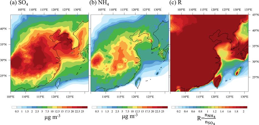
A.-H. Kim et al.: Optimization of the sulfate aerosol hygroscopicity parameter in WRF-Chem                                          261

That is, κi is the volume-weighted average of κj for mode i:         nitrate ions (Seinfeld and Pandis, 2006), and sulfate aerosols
       XJ                                                            appear only in the form of H2 SO4 and (NH4 )2 SO4 . In the cal-
κi ≡         ε κ ,                                            (1)    culation of κSO4 , the proportion of H2 SO4 and (NH4 )2 SO4
         j =1 ij j
                                                                     is determined using the ammonium to sulfate molar ratio
where εij is the volume ratio of chemical j in mode i (=             R = nNH+ /nSO2− , where nNH+ is the molar concentration of
                                                                               4      4               4
Vij /Vtot,i , Vtot,i = Jj=1 Vij , and Vij is the volume of chem-     NH+                      is the molar concentration of SO2−
                      P
                                                                          4 ions, and nSO2− 4
                                                                                                                                  4
ical j in mode i), and κj is the individual hygroscopicity           ions. Generally, sulfate aerosols are completely neutralized
parameter for chemical j . In Eq. (1), the temperature is as-        as (NH4 )2 SO4 under high R conditions (R > 2) and are
sumed to be 298.15 K. The upper end of the κ value for hy-           partially neutralized under low R conditions (R < 2) (Wag-
groscopic species of atmospheric relevance is around 1.40            goner et al., 1967; Fisher et al., 2011). Using R and the
(Petter and Kreidenweis, 2007).                                      Zdanovskii–Stokes–Robinson        relationship (i.e., Vd = Vw +
                                                                     Vtot , Vtot = Jj=1 Vj , where Vd is the droplet volume, Vw is
                                                                                  P
2.3    Limitation of previous κSO4 parameterizations                 the volume of water, and Vj is the volume of the chemical
                                                                     j ), a representative κSO4 is defined as follows:
CCN activation is affected by κ values (e.g., Nenes et al.,
2002; Kristjánsson 2002). H2 SO4 has a κ value that is more          κSO4 = εH2 SO4 κH2 SO4 + ε(NH4 )2 SO4 κ(NH4 )2 SO4 ,           (2)
than 2 times higher than (NH4 )2 SO4 : 1.19 for κH2 SO4 and
0.53 for κ(NH4 )2 SO4 (Clegg and Wexler, 1998; Petters and           where εH2 SO4 is the volume fraction of H2 SO4 in the total
Kredenweis 2007; Good et al., 2010). Such large dispari-             volume of sulfate aerosols (defined as VH2 SO4 /VSO4 , where
ties in the κSO4 between different sulfate species could cause       VH2 SO4 is the volume concentration of H2 SO4 , and VSO4
large variability in the estimation of ERFaci. However, many         is the total volume concentration of sulfate aerosols), and
aerosol modules simplify the physical and chemical charac-           ε(NH4 )2 SO4 is calculated in the same manner for (NH4 )2 SO4
teristics of aerosols, often neglecting some chemical species        (defined as V(NH4 )2 SO4 /VSO4 , where V(NH4 )2 SO4 is the volume
(Kukkonen et al., 2012; Im et al., 2015; Bessagnet et al.,           concentration of (NH4 )2 SO4 ). In this study, we use 1.19 and
2016). Sulfate aerosols are usually prescribed as a single           0.53 to represent κH2 SO4 and κ(NH4 )2 SO4 , respectively (Clegg
species of either H2 SO4 or (NH4 )2 SO4 . Some models con-           and Wexler, 1998; Petters and Kredenweis 2007; Good et al.,
sider H2 SO4 as the representative sulfate aerosol when the          2010). The volume fractions of H2 SO4 and (NH4 )2 SO4 are
neutralization reaction between H2 SO4 and ammonia is not            calculated as follows:
considered or when only the binary sulfuric acid–water nu-
cleation is considered (e.g., Wexler et al., 1994; Kulmala et        (i)       if R = 0, then εH2 SO4 = 1 and ε(NH4 )2 SO4 = 0,
al., 1998; Stier et al., 2006; Kazil and Lovejoy, 2007; Korho-       (ii)      if 0 < R < 2, then
nen et al., 2008; Mann et al., 2010). Some other models con-                                  h                 i m
                                                                                                1 − R2 × nSO2− × ρH 2SO 4
                                                                                                                     H SO
sider (NH4 )2 SO4 as the representative sulfate aerosol when
                                                                                                              4        2 4
studying aerosol–CCN closure (e.g., VanReken et al., 2003),                       εH2 SO4 =                                         (3)
                                                                                                          VSO4
or when including the ternary sulfuric acid–ammonia–water
nucleation process or the neutralization reaction between sul-                    and
                                                                                                              m
fate and ammonia (Kulmala et al., 2002; Napari et al., 2002;                                        R              (NH ) SO
                                                                                                    2 × nSO2−   × ρ(NH 4) 2SO 4
                                                                                                           4          4 2 4
Grell et al., 2005; Elleman and Covert, 2009; Watanabe et                         ε(NH4 )2 SO4 =                                ,
al., 2010). To reduce the uncertainty of ERFaci, more speci-                                                VSO4
ated κSO4 parameters need to be utilized in the calculation of       (iii)     if R > 2, then εH2 SO4 = 0 and ε(NH4 )2 SO4 = 1.
cloud droplet activation process – at least for the two main
sulfate aerosols, H2 SO4 and (NH4 )2 SO4 . Here, we suggest a        Here, m and ρ indicate the molar mass and density of the
new method of representing κSO4 that considers both H2 SO4           specific chemical species, respectively. To be more realistic,
and (NH4 )2 SO4 using the molar ratio of NH+              2−         ammonium bisulfate may also need to be considered: when
                                                  4 to SO4 . We
also suggest an alternative method that utilizes the spatial dis-    the number of SO2−                      +
                                                                                        4 is smaller than NH4 , the sulfates appear
tribution of κSO4 , based on the distinct distribution patterns of   as a mixture of ammonium bisulfates and sulfuric acids, and
NH+            2−                                                    when the number of SO2−                       +
                                                                                              4 is greater than NH4 but not twice
     4 and SO4 over land and sea.                                                    +
                                                                     as large as NH4 , the sulfates appear as a mixture of ammo-
2.4    New parameterization of κSO4                                  nium bisulfates and ammonium sulfates (Nenes et al., 1998;
                                                                     Moore et al., 2011, 2012). For simplicity, however, such par-
H2 SO4 is completely neutralized as (NH4 )2 SO4 when am-             titioning is not considered in this study. As a result, sulfate
monia is abundant (Seinfeld and Pandis, 2006). During the            aerosols are treated as (NH4 )2 SO4 when R is greater than
neutralization process of H2 SO4 , 1 mol of SO2− 4 takes up          two (R > 2) and as H2 SO4 when R is zero (R = 0). This
2 mol of NH+  4 and forms  1 mol  of (NH 4 )2 SO4 . Here, the        method is applicable to the models that consider both NH+    4
assumption is that ammonia neutralizes SO2−  4  ions prior to        and SO2−               +
                                                                             4 ions. If NH4 data are not available in a model, we

https://doi.org/10.5194/gmd-14-259-2021                                                    Geosci. Model Dev., 14, 259–273, 2021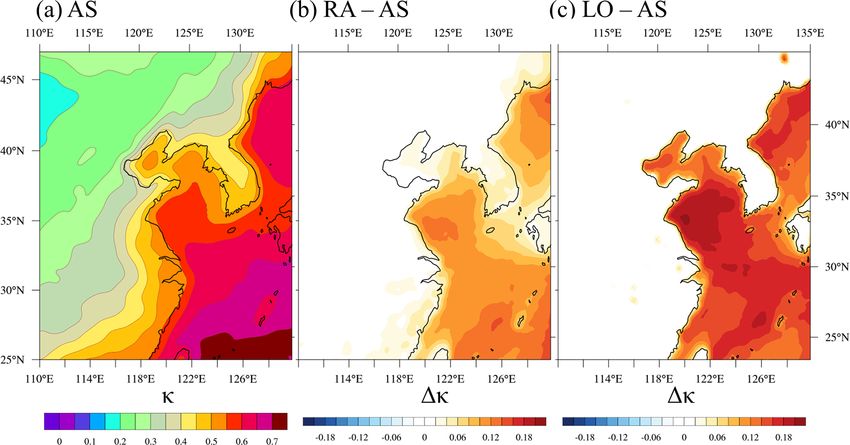
262 A.-H. Kim et al.: Optimization of the sulfate aerosol hygroscopicity parameter in WRF-Chem
suggest an alternative method to represent κSO4 based on the inventories adopt the Model of Emissions of Gases and
typical geographical distribution pattern of sulfate aerosols Aerosols from Nature (MEGAN; Guenther et al., 2006).
available from observations, as discussed below. We conduct four simulations with different κSO4 pa-
Observational studies show the distinctly different distri- rameterizations: (1) AS uses a single κSO4 of 0.53 (i.e.,
bution patterns of the two dominant sulfate aerosol species, κ(NH4 )2 SO4 ), assuming that all sulfate aerosols are completely
i.e., (NH4 )2 SO4 over land and H2 SO4 over sea (Fujita et al., neutralized by ammonium, which is a default setting in
2000; Paulot et al., 2015; Kang et al., 2016; Liu et al., 2017). WRF-Chem; (2) SA uses a single κSO4 of 1.19 (i.e., κH2 SO4 ),
Such distribution patterns are related to the sources of sulfate assuming that all sulfate aerosols are H2 SO4 ; (3) RA applies
and ammonium. In general, sulfate aerosols are emitted from the new κSO4 parameterization that calculates the volume-
land and sea, whereas ammonium is mostly produced from weighted mean κSO4 using the molar ratio of ammonium to
land. Sulfur dioxide is produced from fossil fuel combus- sulfate (R, i.e., Eq. 2); and (4) LO adopts different κSO4 val-
tion, volcanic eruptions, and dimethyl sulfide (DMS) via air– ues for land and sea, assuming that sulfate aerosols are com-
sea exchanges, and then forms sulfate aerosols (Aneja 1990; pletely neutralized as (NH4 )2 SO4 over land and are H2 SO4
Jardin et al., 2015). Wind transportation of pollutants could only over sea (i.e., Eq. 4).
also cause high concentrations of sulfate aerosols over the
sea (Liu et al., 2008). In contrast, ammonium is emitted from
livestock, fertilizer, and vehicles (Sutton et al., 2013; Paulot 4 Results and discussion
et al., 2014; Bishop et al., 2015; Liu et al., 2015; Stritzke et
al., 2015); therefore, it is concentrated mostly on land. Am- 4.1 Distribution of sulfate and ammonium
monium is usually not abundant enough to fully neutralize
H2 SO4 in the marine boundary layer (Paulot et al., 2015; Ce- The simulated sulfate and ammonium distributions are com-
burnis et al., 2016). Thus, when ammonium information is pared with the observational data that were measured on-
not available, the κSO4 can be alternatively estimated by con- board the NASA DC-8 aircraft during the KORUS–AQ cam-
sidering the land and sea fractions as follows: paign (https://www-air.larc.nasa.gov/missions/korus-aq/,
last access: 18 July 2019) in and around the Korean Penin-
κSO4 = f × κSO4 ,land + (1 − f ) × κSO4 ,sea , (4) sula in May and June of 2016. The measurements were taken
within the boundary layer. The mass concentration of sulfate
where f represents the fraction of land at each grid point; and ammonium were obtained using the method described
unity means entire land, zero means entire sea, and the value in Dibb et al. (2003).
in between represents the fraction of land at the grid points in In Fig. 1, the mass concentration of sulfate and ammonium
coastal areas. κSO4 ,land and κSO4 ,sea represent κSO4 over land simulated by AS are compared with the KORUS-AQ aircraft
and sea, respectively (i.e., κSO4 ,land = κ(NH4 )2 SO4 = 0.53 and observations (OBS) following the flight track. The simulated
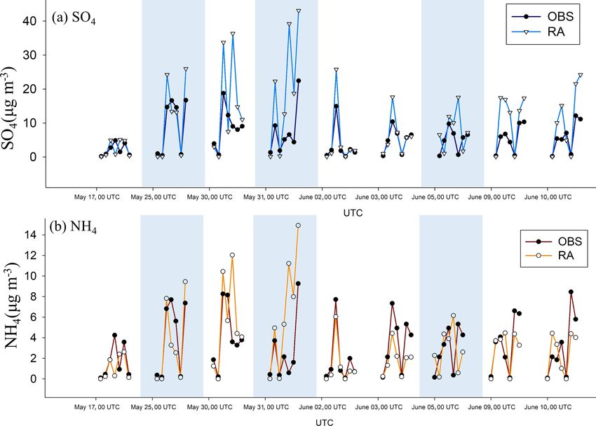
κSO4 ,sea = κH2 SO4 = 1.19). sulfate shows a positive bias but has a high temporal correla-
tion with OBS (r = 0.78). The simulated ammonium is less
biased than sulfate but indicates a moderate temporal corre-
3 Experimental setup lation with OBS (r = 0.58). Overall, it seems reasonable to
state that the WRF-Chem model can calculate the distribu-
Model simulations are carried out for 36 d from 00:00 UTC tion of sulfate aerosols well enough.
on 10 May to 00:00 UTC on 15 June 2016 and the first 5 d Figure 2 shows the 30 d averaged mass concentration of
are used as spin-up. Observational data for sulfate aerosols sulfate and ammonium and the molar ratio (R) of ammonium
and CCN during this period were obtained from the KORUS- to sulfate over the model domain. During the KORUS-AQ
AQ campaign, and they indicated that sulfate aerosols were campaign period, high-pressure systems often covered East
widely distributed throughout East Asia due to the stagnation China and the Yellow Sea, and this led to stagnating sulfate
of high-pressure systems and the transportation of pollutants and ammonium concentrations. However, sulfate and ammo-
from China. The domain covers East Asia (i.e., 2700 km × nium are distributed differently due to different sources. Pol-
2700 km; 20–50◦ N, 105–135◦ E) with 18 km grid spacing lutants emitted from the Asian continent are often transported
and 50 vertical levels from sea level pressure to 100 hPa. The by westerly and southerly winds. Sulfate is highly concen-
initial and boundary conditions are provided by the National trated in China and the northern part of the Yellow Sea, and
Center for Environment Prediction–Climate Forecast System DMS emission from the sea also contributes to the formation
Reanalysis (NCEP–CFSR; Saha et al., 2014). The 4DDA of sulfate aerosols over the sea. Ammonium is widely dis-
(Four-Dimensional Data Assimilation) analysis nudging is tributed throughout China due to the use of fertilizers over
used. Anthropogenic emission inventories are obtained from farmlands (Paulot et al., 2014; Van Damme et al., 2014;
the Emissions Database for Global Atmospheric Research– Warner et al., 2017). The concentration of ammonium is gen-
Hemispheric Transport of Air Pollution (EDGAR–HTAP; erally low over the sea, but it is high over the northern part of
Janssens-Maenhout et al., 2015). Natural source emission the Yellow Sea due to wind transport.
Geosci. Model Dev., 14, 259–273, 2021 https://doi.org/10.5194/gmd-14-259-2021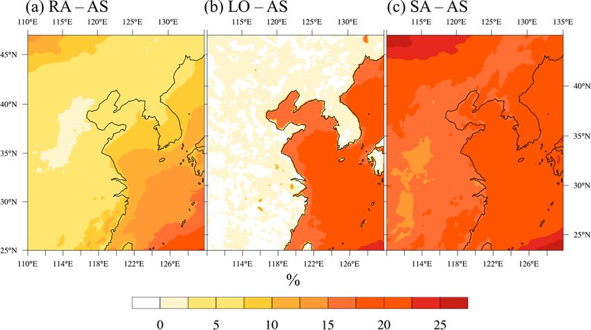
A.-H. Kim et al.: Optimization of the sulfate aerosol hygroscopicity parameter in WRF-Chem                                       263

Figure 1. Time variation of the mass concentrations of (a) sulfate and (b) ammonium measured by the NASA DC-8 aircraft (OBS, black
line) and simulated by RA (colored line). The blue shaded regions denote the time over the sea.

Figure 2. The 30 d averaged (00:00 UTC on 16 May to 00:00 UTC on 15 June 2016) spatial distribution of the mass concentrations of (a)
sulfate and (b) ammonium, and (c) the molar ratio of ammonium to sulfate (R) at the surface, from AS.

   The distribution of R is associated with the distribution of      4.2   Distribution of κ
sulfate and ammonium (Fig. 2). In general, R is high (R > 2)
over land on account of the high anthropogenic emissions of          Figure 3 shows the average κ of the accumulation-mode
continental ammonium, and R is low (R < 2) over remote               aerosols in AS and the difference between RA and AS and
seas because the ammonium concentration is small. How-               between LO and AS.
ever, high R is also shown over the Yellow Sea in Fig. 2. This          The accumulation mode is selected because sulfate
is because the ammonium concentration increases when the             aerosols are dominant in this mode. AS simulates κ values
westerlies carry continental pollutants over the Yellow Sea          that are roughly consistent with the observed mean κ values
during the simulation period. Based on the distribution of R,        in the literature (i.e., κ over land is about 0.3 and κ over sea
sulfate aerosols are expected to be almost completely neu-           is about 0.7; Andreas and Rosenfeld, 2008), but it varies sig-
tralized over land (e.g., (NH4 )2 SO4 ) and partially neutralized    nificantly between land and sea. The κ over land is expected
over sea ((NH4 )2 SO4 + H2 SO4 ).                                    to be lower than the κ over sea because continental aerosols

https://doi.org/10.5194/gmd-14-259-2021                                                   Geosci. Model Dev., 14, 259–273, 2021
264                          A.-H. Kim et al.: Optimization of the sulfate aerosol hygroscopicity parameter in WRF-Chem

Figure 3. (a) Spatial distribution of the hygroscopicity parameter (κ) in the accumulation mode simulated by AS, and the difference in κ (b)
between RA and AS and (c) between LO and AS, at the surface.

usually include more hydrophobic aerosol species such as                   The model simulations capture the temporal variation of
black carbon and organic carbon from industry, whereas mar-             fCCN well (r ≈ 0.7 for the linear correlation with OBS;
itime aerosols consist mainly of hygroscopic substances, i.e.,          Fig. 4).
sea salt and non-sea salt sulfates originating from DMS. The               However, fCCN values are underestimated mainly due to
variation in κ is also influenced by chemical reactions and             the underestimation of CCN concentrations. The average
meteorological factors, i.e., wind transportation of aerosols           aerosol (CN) number concentrations for the flight track in
and scavenging of aerosols due to precipitation, as well as             all simulations (AS, SA, RA, and LO) and the actual ob-
gravitational settling.                                                 served values during the flight are 5934 and 5794 cm−3 , re-
   Compared with AS, RA and LO show a pronounced dif-                   spectively. Thus, unlike Georgiou et al. (2018), who showed
ference in κ over sea (Fig. 3b, c). That is, RA and LO pro-             that WRF-Chem coupled with MADE/SORGAM tended to
duce significantly higher κ over the sea than AS does be-               overestimate aerosol number concentrations, our simulations
cause the ammonium concentration is not sufficient to neu-              only slightly overestimated aerosol number concentrations.
tralize sulfate completely over the sea (i.e., R < 2). RA pre-          The average CCN number concentration at 0.6 % supersatu-
dicts slightly higher continental κ following the coastal re-           ration for the AS, RA, and LO simulations are 982, 1027, and
gions than AS because R occasionally becomes low due to                 1057 cm−3 , respectively, but the observation was 2154 cm−3 .
the intrusion of maritime air masses that have very low con-            Such underestimated CCN concentrations seem to be due to
centrations of ammonium. Maritime κ of RA is lower than                 the systematic error in WRF-Chem. As discussed in Tuc-
that of LO because the transportation of continental pollu-             cella et al. (2015), the uncertainty of the updraft velocity pa-
tants increases the portion of ammonium over the Yellow sea.            rameterization and bulk hygroscopicity of aerosols lead to
                                                                        an underestimation of the CCN concentration and CCN effi-
4.3   CCN activation                                                    ciency (CCN/CN) by a factor of 1.5 and 3.8, respectively.
                                                                        Nevertheless, over land, AS, RA, and LO simulate simi-
                                                                        lar values of fCCN because continental sulfate aerosols are
According to the Köhler theory, changes in κ directly in-
                                                                        generally expected to be a fully neutralized form of sulfate
fluence CCN activation. In this study, the CCN activation
                                                                        (i.e., (NH4 )2 SO4 ). This was not the case over sea. During
rate (fCCN ) is defined as the ratio of the CCN number
                                                                        KORUS-AQ, the aircraft passed over the Yellow Sea on 22
concentration at 0.6 % supersaturation to the total aerosol
                                                                        and 25 May 2016 (blue shading in Fig. 4). On this occasion,
number concentration. Simulated fCCN is compared with
                                                                        LO simulates the highest fCCN over the sea among all simu-
the aircraft measurements during the KORUS-AQ campaign
                                                                        lations because LO uses the prescribed κSO4 value of κH2 SO4
(OBS). During this campaign, aerosol and CCN number
                                                                        over sea. RA simulates slightly lower fCCN over the sea be-
concentrations were measured by a condensation particle
                                                                        cause transportation of continental pollutants over the sea can
counter (CPC; TSI, 3010) and a CCN counter (CCNC; DMT,
                                                                        be taken into account, as observed during the KORUS-AQ
CCN-100), respectively (Park et al., 2020). The CPC mea-
                                                                        campaign. The transported air pollutants increase the ammo-
sures the number concentration of aerosols larger than 10 nm
                                                                        nium concentration over the sea, neutralize H2 SO4 , reduce
in diameter, and the CCNC measures the CCN number con-
                                                                        the hygroscopicity of sulfate aerosols, and consequently de-
centration at 0.6 % supersaturation.

Geosci. Model Dev., 14, 259–273, 2021                                                      https://doi.org/10.5194/gmd-14-259-2021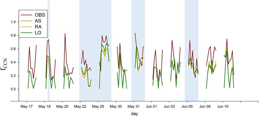
A.-H. Kim et al.: Optimization of the sulfate aerosol hygroscopicity parameter in WRF-Chem                                        265

Figure 4. Time variation in the CCN activation fractions at 0.6 % supersaturation (fCCN ) measured by the NASA DC-8 aircraft (OBS) and
simulated by AS, RA, and LO. The blue shaded regions denote the time over the sea.

crease fCCN . Simulated fCCN in RA has a high spatiotem-             4.4   Cloud microphysical properties
poral correlation with the observation over the Yellow Sea
(i.e., 0.83), whereas AS shows a rather lower correlation (i.e.,
                                                                     Different κSO4 parameterizations affect simulated cloud mi-
0.65). Such difference stems from the fact that R values vary
                                                                     crophysical properties. Figure 6 shows the relative differ-
significantly over the Yellow sea due to the transportation of
                                                                     ences in the simulated column-integrated cloud droplet num-
anthropogenic chemicals by westerlies, and such variability
                                                                     ber concentration (CDNC) in RA, LO, and SA from AS.
is taken into account in RA. This improvement highlights
                                                                     All three produce higher κSO4 values than AS and, therefore,
the importance of appropriate chemical representation in at-
                                                                     simulate higher CDNCs. However, the differences in CDNC
mospheric models. Compared with the RA and LO simula-
                                                                     do not exactly correspond to the differences in fCCN (Fig. 5)
tions, AS predicts the lowest fCCN because the lowest κSO4
                                                                     because cloud droplet activation is also affected by in-cloud
(= κ(NH4 )2 SO4 ) is prescribed over sea as well as over land.
                                                                     supersaturation and other meteorological factors. SA simu-
   We conducted a reliability test that has been often used
                                                                     lates higher CDNC than AS over both land and sea, but RA
to evaluate the performance of air quality models. Kumar
                                                                     and LO simulate higher CDNC mostly only over sea. RA and
et al. (1993) proposed the following three criteria for judg-
                                                                     LO produce similar CDNC distributions over the Yellow Sea
ing model reliability: (1) the normalized mean squared er-
                                                                     (compare Fig. 6a and b) although RA produces smaller fCCN
ror (NMSE) below 0.5; (2) the fractional bias (defined as
                                                                     than LO (compare Fig. 5a and b). As in Moore et al. (2011),
2 × OBS−sim , where OBS indicates the observed values, sim           the reason for this may be that the sensitivity on fCCN de-
      OBS+sim
indicates the simulated values, and the bar above the sym-           creases so much because supersaturation is so high that most
bols indicates the average) between −0.5 and 0.5; and (3)            aerosols can act as CCN regardless of their critical super-
the ratio of the model values to the observed values (defined        saturation. That is, the supersaturation over the Yellow Sea is
as sim/OBS) between 0.5 and 2.0. These values for AS, RA,            high enough to activate most aerosols to cloud droplets. Over
and LO are compared in Table 3. It indicates that RA and LO          land, RA simulates higher CDNC (up to 12 %) than AS in
satisfy all three criteria, but AS does not satisfy two of the       southeast China and the Korean Peninsula, but LO simulates
three criteria as it predicts a rather high normalized NMSE          CDNC similar to AS. The results of RA seem to be related to
and fractional bias. Between RA and LO, LO seems some-               the dilution of ammonium concentrations along the coastal
what closer to the observations than RA, but the difference is       land regions due to the intrusion of maritime air. However,
small for these calculations.                                        such variation in ammonium cannot be taken into account in
   The variation in κSO4 almost directly influences the change       LO.
in the column-integrated fCCN (Fig. 5).                                 Overall, high CDNCs in RA, LO, and SA (Table 1) re-
   RA predicts higher fCCN than AS over the coastal land re-         sult in less precipitation but larger liquid water path (LWP),
gions because the occasionally very low ammonium concen-             compared with AS (Table 2). Precipitation reduction is more
tration lowers R and affects the CCN activation. Meanwhile,          pronounced over sea because of larger relative differences in
SA prescribes κSO4 value 2 times as high as AS does and              CDNC. These results agree well with some previous stud-
produces about 20 % higher fCCN values.                              ies – i.e., high CDNCs suppress local precipitation, prolong
                                                                     cloud lifetime, and consequently increase net LWP, which
                                                                     is known as the cloud lifetime effect (Albrecht, 1989). Ob-
                                                                     viously, SA, which assumes sulfate aerosols are all H2 SO4

https://doi.org/10.5194/gmd-14-259-2021                                                    Geosci. Model Dev., 14, 259–273, 2021
266 A.-H. Kim et al.: Optimization of the sulfate aerosol hygroscopicity parameter in WRF-Chem
Figure 5. Percentage difference in the column-integrated CCN activation fraction at 0.6 % supersaturation (fCCN ) in AS and sensitivity
simulations: (a) RA – AS, (b) LO – AS, and (c) SA – AS.
Figure 6. Same as Fig. 5 except for the cloud droplet number concentration (CDNC).
particles, produces the highest CDNC and also the largest Table 1. Domain-averaged differences (=
sensitivity simulation-AS
×
AS
differences in all other properties in Table 2. Less rainwa- 100 %) of the CCN activation fraction at 0.6 % supersaturation
ter in SA than in any other simulations may also imply that (fCCN ) and the cloud droplet number concentration (CDNC) in
precipitation scavenging of aerosols was less efficient and, percent. The data are averaged from 00:00 UTC on 15 May to
therefore, that more aerosols (CCN) were retained to pro- 00:00 UTC on 15 June.
duce more cloud drops and a longer cloud lifetime. On aver-
age, SA has 103 cm−3 more aerosols over sea and 116 cm−3 RA – AS LO – AS SA – AS
more aerosols over land than LO. These surplus aerosols cer- Land Ocean Land Ocean Land Ocean
tainly have the potential to simulate a higher number of CCN
fCCN 6 13 1 19 18 22
in SA than in LO.
(%)
For the same LWP condition, high CDNC induces small
CDNC 7 20 1 21 14 24
effective radii (re ). RA, LO, and SA simulate smaller re than (%)
AS, and the maximum difference in re amounts to 1.46, 1.38,
and 1.48 µm, respectively. However, the domain-averaged
differences in re are not as substantial as the differences in
Geosci. Model Dev., 14, 259–273, 2021 https://doi.org/10.5194/gmd-14-259-2021A.-H. Kim et al.: Optimization of the sulfate aerosol hygroscopicity parameter in WRF-Chem 267
Table 2. Domain-averaged water budgets of AS and their differences from other simulations. The data are averaged from 00:00 UTC on
15 May to 00:00 UTC on 15 June. Rainwater in this study refers to the liquid phase of water that has a potential to become rainfall in the
model. LWP stands for liquid water path, and IWP stands for ice water path.
AS RA – AS LO – AS SA – AS
Land Ocean Land Ocean Land Ocean Land Ocean
Rainwater (g m−2 ) 21.6 39.4 −0.32 −0.60 −0.02 −0.64 −0.52 −0.73
LWP (g m−2 ) 45.7 78.4 0.40 1.41 0.08 1.45 0.73 1.69
IWP (g m−2 ) 9.34 11.2 0.05 0.08 0.02 0.07 0.08 0.09
re (µm) 6.13 10.3 −0.02 −0.11 0.00 −0.11 −0.04 −0.12
Table 3. Values of the three criteria suggested in Kumar et al. (1993).
AS RA LO
NMSE < 0.5 0.53 0.48 0.43
−0.5 < fractional bias (= 2 × OBS−sim ) < 0.5 0.54 0.50 0.46
OBS+sim
0.5 < ratio (= sim/OBS) < 2 0.59 0.65 0.65
other cloud microphysical properties (Table 2). This may be cloud fraction exerts a large CRE cooling, so the impact of
related to somewhat larger LWPs in RA, LO, and SA than the new parameterization of κSO4 on CRE could be substan-
in AS as well as the sufficient water supply during droplet tial under large cloud fraction conditions. Note that CRE is
growth. All simulations in this study have high water vapor similar over land and over the sea in the latitude band from
path (WVP) conditions (WVP > 30 kg m−2 ) throughout the 25 to 28◦ N in AS (Fig. 7a), but the CRE differences between
whole domain. According to Qiu et al. (2017), cloud droplets RA, LO and SA, and AS are much higher over the sea than
have low competition for water vapor and a high chance over land (Fig. 7b, c, d). Such an enhanced cooling effect
of collision–coalescence under high WVP conditions (i.e., over the sea can be explained by increases in CDNC (Fig. 6)
WVP > 1.5 cm or 15 kg m−2 ). If LWP is similar, the re dif- and, somewhat, by increases in LWP (Table 2). According to
ference could be larger among the simulations than those that some previous studies, the contribution of CDNC and LWP
are shown herein. to CRE could be larger than 56 % (Sengupta et al., 2003;
Goren and Rosenfeld, 2014).
4.5 Cloud radiative effects
Cloud microphysical properties determine cloud optical 5 Summary and conclusions
properties and, therefore, control the cloud radiative effects.
For a fixed LWP, high CDNC is usually associated with This study introduces a new hygroscopicity parameteriza-
low re but high cloud optical thickness. Then optically thick tion method for sulfate aerosols in the WRF-Chem model
clouds reflect more sunlight and strengthen the cloud radia- and demonstrates the impacts of different κSO4 parameteri-
tive cooling effect at the top of the atmosphere (TOA), which zation on simulating cloud microphysical properties in East
is known as the cloud albedo effect (Twomey, 1974). We Asia. The new κSO4 parameterization considers the composi-
calculate the cloud radiative effect at the TOA (CRE) by tion effect of H2 SO4 and (NH4 )2 SO4 , using the molar ratio
subtracting the clear-sky downward radiation from the net of ammonium to sulfate, R. We also suggest an alternative
all-sky downward radiation (including clouds) (Hartmann, κSO4 parameterization – κ(NH4 )2 SO4 for land and κH2 SO4 for
2016). sea – which utilizes information on the typical observed geo-
RA, LO, and SA simulate optically thicker clouds that graphical distribution of sulfate aerosols, in cases where am-
reflect more sunlight and exert stronger cooling effects at monium data are not available. The performance of the new
the TOA than AS (Fig. 7). For the domain average, the dif- κSO4 parameterizations was evaluated by comparing it with
ferences in CRE for RA, LO, and SA from AS amount to observational data obtained from a field campaign in East
about −1.7, −1.5, and −2.1 W m−2 , respectively. These dif- Asia, and it was demonstrated that the new parameteriza-
ferences are most pronounced over sea (Fig. 7b, c, d). Such tions could produce more reliable aerosol and CCN concen-
pronounced difference over sea may be affected by the large trations than the previous method, which used a single κSO4
cloud fraction around the East China Sea due to the East value (i.e., κ(NH4 )2 SO4 ). It should be noted that the κ values
Asian summer monsoon (Pan et al., 2015). That is, a large of 0.53 and 1.19 for (NH4 )2 SO4 and H2 SO4 that we used in
https://doi.org/10.5194/gmd-14-259-2021 Geosci. Model Dev., 14, 259–273, 2021268 A.-H. Kim et al.: Optimization of the sulfate aerosol hygroscopicity parameter in WRF-Chem Figure 7. The simulated 30 d averaged (00:00 UTC on 16 May to 00:00 UTC on 15 June 2016) cloud radiative effect (CRE) for (a) AS and the differences (1CRE) between (b) RA and AS, (c) LO and AS, and (d) SA and AS. this study were derived from humidified tandem differential κSO4 (i.e., κ(NH4 )2 SO4 ) or an empirical relationship between mobility analyzer (HTDMA) measurements, instead of being (NH4 )2 SO4 and CCN to calculate CCN activation (Boucher derived from CCN, which were 0.61 and 0.90, respectively and Anderson, 1995; Kiehl et al., 2000). All in all, the new (Petters and Kreidenweis, 2007). If CCN-derived κ values κSO4 parameterization is capable of considering the varia- were used, CDNC would generally have decreased because tion in κSO4 and simulates more reliable results, compared κ became lower and the contrast between (NH4 )2 SO4 and with the previous method using a single κSO4 value in the H2 SO4 would have been decreased to a certain degree. In calculation of cloud microphysical properties. Many atmo- the context of cloud droplet activation, CCN-derived κ val- spheric models neglect the differences in hygroscopicity be- ues might be more appropriate to use because they would tween H2 SO4 and (NH4 )2 SO4 for simplicity. However, this be measured under cloudy (i.e., supersaturated) conditions. could result in large uncertainties in estimating CRE, espe- However, in this study, we try to manifest the effect of dif- cially in East Asia, as demonstrated in our results. ferent κ values of the two major sulfate species, and this was Therefore, we propose this new parameterization of κSO4 the main reason for choosing HTDMA-derived κ values that that considers both of the dominant sulfate aerosols, H2 SO4 show a greater difference between (NH4 )2 SO4 and H2 SO4 , and (NH4 )2 SO4 , when investigating the effects of sulfate instead of CCN-derived values that show a smaller differ- aerosols on climate – especially for East Asia, which shows ence. distinctly different emission patterns over land and sea. The The effect of the new κSO4 parameterizations is indi- new parameterizations are applicable to calculate CCN ac- cated as substantially different cloud microphysical proper- tivation without additional treatments of the chemical reac- ties, especially over the sea (about 20 % increases in CDNC). tions and computational expenses. The new parameterization The increases in CDNC suppress local precipitation, prolong introduced in this study is expected to work effectively in cloud lifetime, and consequently reflect more sunlight, i.e., a the domain where land and sea are almost evenly distributed larger cooling effect (about 1.5 W m−2 ), than the simulation or in the regions with a varying distribution of ammonium with the original κSO4 parameterization in WRF-Chem that to sulfate molar ratio. However, we only tested the perfor- assumes κSO4 = κ(NH4 )2 SO4 for all sulfate aerosols. These re- mance of the new κSO4 parameterization in East Asia due to sults indicate that the estimated cloud radiative forcing due the limited amount of observational data available to validate to aerosol–cloud interactions can vary significantly with dif- the performance of CCN activation. Therefore, further stud- ferent κSO4 parameterizations. ies are needed for different regions where observational data The importance of oceanic sulfate aerosols on radiative are available to confirm the reliability of our new parameter- forcing is highlighted in recent studies which suggested that ization. DMS (precursor of oceanic sulfate aerosols) emissions sig- In this study, we did not discuss other important aerosol nificantly contribute to the total radiative forcing due to species. For instance, the proportion of mass concentrations aerosol–cloud interactions (Carslaw et al., 2013; Yang et al., of nitrate ions are almost as large as sulfate ions (Zhang et 2017). The new κSO4 parameterizations could be more ap- al., 2012; Moore et al., 2012), and nitrate also has spatiotem- propriate for studying the effects of oceanic sulfate aerosols porally varying hygroscopicity due to the complex chemi- on climate, compared with other approaches that use a single cal reactions with other chemicals, i.e., ammonium, sodium, Geosci. Model Dev., 14, 259–273, 2021 https://doi.org/10.5194/gmd-14-259-2021
A.-H. Kim et al.: Optimization of the sulfate aerosol hygroscopicity parameter in WRF-Chem                                               269

and calcium. In this work, we only made changes in the rep-              Review statement. This paper was edited by Samuel Remy and re-
resentation of sulfate aerosol species and did not alter any             viewed by Richard Moore and one anonymous referee.
other chemical processes, and we find that the amount of ni-
trate and sea salt aerosols in the AS, RA, and LO simulations
were similar. Perhaps this implies that the different treatment
                                                                         References
of sulfate aerosols did not significantly affect nitrate and sea
salt aerosols. However, it is difficult to estimate how the pres-        Abdul-Razzak, H. and Ghan, S. J.: A parameterization of aerosol ac-
ence of nitrate and sea salt aerosols impacted the results in              tivation: 2. Multiple aerosol types, J. Geophys. Res., 105, 6837–
our simulations. Future studies may need to address such im-               6844, https://doi.org/10.1029/1999jd901161, 2000.
portant issue in more detail.                                            Abdul-Razzak, H., Ghan, S. J., and Rivera-Carpio, C.: A parameter-
                                                                           ization of aerosol activation. Part I: Single aerosol type, J. Geo-
                                                                           phys. Res., 103, 6123–6131, https://doi.org/10.1029/97jd03735,
Code availability. The original WRF-Chem v3.8.1 source code is             1998.
available at https://www2.mmm.ucar.edu/wrf/users/download/get_           Ackermann, I. J., Hass, H., Memmesheimer, M., Ebel, A.,
sources.html (last access: 16 August 2019, Grell et al., 2005; Fast et     Binkowski, F. S., and Shankar U.: Modal aerosol dynamics
al., 2006; Skamarock et al., 2008; Peckham et al., 2011). The opti-        model for Europe: Development and first applications, At-
mized sulfate aerosol hygroscopicity parameter code is available at        mos. Environ., 32, 2981–2999, https://doi.org/10.1016/s1352-
https://doi.org/10.5281/zenodo.3899838 (Kim, 2020).                        2310(98)00006-5, 1998.
                                                                         Albrecht, B. A.: Aerosols, cloud microphysics and
                                                                           fractional     cloudiness,      Science,      245,     1227–1230,
Data availability. The National Center for Environment                     https://doi.org/10.1126/science.245.4923.1227, 1989.
Prediction–Climate Forecast System Reanalysis (NCEP–CFSR)                Al-Saadi, J., Carmichael, G., Crawford, J., Emmons, L., Song,
data for initial and boundary conditions were obtained from                C. K., Chang, L. S., Lee, G., Kim, J., and Park, R.: NASA
https://rda.ucar.edu/datasets/ds093.1/ (last access: 16 August 2019,       contributions to KORUS-AQ: An international cooperative
Saha et al., 2014). Anthropogenic emission inventories were                air quality field study in Korea, NASA White Pap., Virginia,
obtained from the Emissions Database for Global Atmospheric                USA, available at: https://espo.nasa.gov/sites/default/files/
Research–Hemispheric Transport of Air Pollution (EDGAR–                    documents/White%20paper%20outlining%20NASA%e2%80%
HTAP; Janssens-Maenhout et al., 2015). The data measured from              99s%20contribution%20to%20KORUS-AQ_0.pdf (last access:
the DC-8 aircraft during the KORUS–AQ campaign are available               14 January 2021), 2016.
at https://www-air.larc.nasa.gov/missions/korus-aq/ (last access:        Andreae, M. O. and Rosenfeld, D.: Aerosol-cloud-precipitation
18 July 2019).                                                             interactions. Part 1. The nature and sources of cloud-active
                                                                           aerosols, Earth-Sci. Rev., 89, 13–41, 2008.
                                                                         Aneja, V. P.: Natural sulfur emissions into the atmo-
                                                                           sphere. J. Air Waste Manag. Assoc., 40, 469–476,
Author contributions. AHK constructed the idea, designed the op-
                                                                           https://doi.org/10.1080/10473289.1990.10466701, 1990.
timization method, and wrote the first draft of the paper. SSY ac-
                                                                         Baró, R., Jiménez-Guerrero, P., Balzarini, A., Curci, G., Forkel,
quired funding, supervised the whole study, and edited the paper.
                                                                           R., Grell, G., Hirtl, M., Honzak, L., Langer, M., Pérez, J. L.,
DYC participated in the construction of the idea, the development
                                                                           Pirovano, G., San José, R., Tuccella, P., Werhahn, J., and Žabkar,
of the optimization method, and edited the paper. MP provided the
                                                                           R.: Sensitivity analysis of the microphysics scheme in WRF-
KORUS-AQ campaign data and edited the paper.
                                                                           Chem contributions to AQMEII phase 2, Atmos. Environ., 115,
                                                                           620–629, https://doi.org/10.1016/j.atmosenv.2015.01.047, 2015.
                                                                         Bessagnet, B., Pirovano, G., Mircea, M., Cuvelier, C., Aulinger, A.,
Competing interests. The authors declare that they have no conflict        Calori, G., Ciarelli, G., Manders, A., Stern, R., Tsyro, S., Gar-
of interest.                                                               cía Vivanco, M., Thunis, P., Pay, M.-T., Colette, A., Couvidat,
                                                                           F., Meleux, F., Rouïl, L., Ung, A., Aksoyoglu, S., Baldasano, J.
                                                                           M., Bieser, J., Briganti, G., Cappelletti, A., D’Isidoro, M., Fi-
Acknowledgements. This work was funded by the Korea Me-                    nardi, S., Kranenburg, R., Silibello, C., Carnevale, C., Aas, W.,
teorological Administration Research and Development Program               Dupont, J.-C., Fagerli, H., Gonzalez, L., Menut, L., Prévôt, A. S.
(grant no. KMI2018-03511). Dong Yeong Chang acknowledges                   H., Roberts, P., and White, L.: Presentation of the EURODELTA
support from the Ministry of Education of the Republic of Korea            III intercomparison exercise – evaluation of the chemistry trans-
and the National Research Foundation of Korea (grant no. NRF-              port models’ performance on criteria pollutants and joint anal-
2019R1I1A1A01063751).                                                      ysis with meteorology, Atmos. Chem. Phys., 16, 12667–12701,
                                                                           https://doi.org/10.5194/acp-16-12667-2016, 2016.
                                                                         Bishop, G. A. and Stedman, D. H.: Reactive Nitrogen Species
Financial support. This research has been supported by the Ko-             Emission Trends in Three Light-/Medium-Duty United
rea Meteorological Administration Research and Development Pro-            States Fleets, Environ. Sci. Technol., 49, 11234–11240,
gram (grant no. KMI2018-03511).                                            https://doi.org/10.1021/acs.est.5b02392, 2015.
                                                                         Boucher, O. and Anderson, T. L.: General circulation model assess-
                                                                           ment of the sensitivity of direct climate forcing by anthropogenic

https://doi.org/10.5194/gmd-14-259-2021                                                        Geosci. Model Dev., 14, 259–273, 2021
270 A.-H. Kim et al.: Optimization of the sulfate aerosol hygroscopicity parameter in WRF-Chem
sulfate aerosols to aerosol size and chemistry, J. Geophys. Res., cleation and nucleation mode processes, J. Geophys. Res., 114,
100, 26117–26134, https://doi.org/10.1029/95JD02531, 1995. D11207, https://doi.org/10.1029/2009JD012187, 2009.
Boucher, O., Randall, D., Artaxo, P., Bretherton, C., Feingold, G., Fast, J. D., Gustafson, W. I. Jr, Easter, R. C., Zaveri, R. A., Barnard,
Forster, P., Kerminen, V.-M., Kondo, Y., Liao, H., Lohmann, U., J. C., Chapman, E. G., and Grell, G. A.: Evolution of ozone, par-
Rasch, P., Satheesh, S. K., Sherwood, S., Stevens, B., and Zhang, ticulates, and aerosol direct forcing in an urban area using a new
X. Y.: Clouds and Aerosols, in: Climate Change 2013: The Phys- fully coupled meteorology, chemistry, and aerosol model, J. Geo-
ical Science Basis. Contribution of Working Group I to the Fifth phys. Res., 111, D21305, https://doi.org/10.1029/2005jd006721,
Assessment Report of the Intergovernmental Panel on Climate 2006.
Change, edited by: Stocker, T. F., Qin, D., Plattner, G.-K., Tig- Fisher, J. A., Jacob, D. J., Wang, Q., Bahreini, R., Carouge,
nor, M., Allen, S. K., Boschung, J., Nauels, A., Xia, Y., Bex, C. C., Cubison, M. J., Dibb, J. E., Diehl, T., Jimenez,
V., and Midgley, P. M., Cambridge University Press, Cambridge, J. L., Leibensperger, E. M., Lu, Z., Meinders, M. B. J.,
United Kingdom and New York, NY, USA, 2013. Pye, H. O. T., Quinn, P. K., Sharma, S., Streets, D. G.,
Carslaw, K. S., Lee, L. A., Reddington, C. L., Pringle, K. J., Rap, van Donkelaar, A., and Yantosca, R. M.: Sources, distri-
A., Forster, P. M., Mann, G. W., Spracklen, D. V., Woodhouse, bution, and acidity of sulfate–ammonium aerosol in the
M. T., Regayre, L. A., and Pierce, J. R.: Large contribution of Arctic in winter–spring, Atmos. Environ., 45, 7301–7318,
natural aerosols to uncertainty in indirect forcing, Nature, 503, https://doi.org/10.1016/j.atmosenv.2011.08.030, 2011.
67–71, https://doi.org/10.1038/nature12674, 2013. Fountoukis, C. and Nenes, A.: Continued development
Ceburnis, D., Rinaldi, M., Ovadnevaite, J., Martucci, G., Giu- of a cloud droplet formation parameterization for
lianelli, L., and O’Dowd, C. D.: Marine submicron aerosol gradi- global climate models, J. Geophys. Res., 110, D11212,
ents, sources and sinks, Atmos. Chem. Phys., 16, 12425–12439, https://doi.org/10.1029/2004JD005591, 2005.
https://doi.org/10.5194/acp-16-12425-2016, 2016. Fujita, S.-I., Takahashi, A., Weng, J.-H., Huang, L.-F., Kim, H.-
Chang, D., Lelieveld, J., Tost, H., Steil, B., Pozzer, A., and Yoon, K., Li, C.-K., Huang, F. T. C., and Jeng, F.-T.: Precipita-
J.: Aerosol physicochemical effects on CCN activation simulated tion chemistry in East Asia, Atmos. Environ., 34, 525–537,
with the chemistry-climate model EMAC, Atmos. Environ., 162, https://doi.org/10.1016/S1352-2310(99)00261-7, 2000.
127–140, https://doi.org/10.1016/j.atmosenv.2017.03.036, 2017. Gasteiger, J. and Wiegner, M.: MOPSMAP v1.0: a versatile
Chang, J. S., Binkowski, F. S., Seaman, N. L., McHenry, J. N., tool for the modeling of aerosol optical properties, Geosci.
Samson, P. J., Stockwell, W. R., Walcek, C. J., Madronich, S., Model Dev., 11, 2739–2762, https://doi.org/10.5194/gmd-11-
Middleton, P. B., Pleim, J. E., and Lansford, H. H.: The re- 2739-2018, 2018.
gional acid deposition model and engineering model, State-of- Georgiou, G. K., Christoudias, T., Proestos, Y., Kushta, J., Hadjini-
Science/Technology, Report 4, National Acid Precipitation As- colaou, P., and Lelieveld, J.: Air quality modelling in the summer
sessment Program, Washington, D.C., 1989. over the eastern Mediterranean using WRF-Chem: chemistry and
Chapman, E. G., Gustafson Jr., W. I., Easter, R. C., Barnard, aerosol mechanism intercomparison, Atmos. Chem. Phys., 18,
J. C., Ghan, S. J., Pekour, M. S., and Fast, J. D.: Coupling 1555–1571, https://doi.org/10.5194/acp-18-1555-2018, 2018.
aerosol-cloud-radiative processes in the WRF-Chem model: In- Ghan, S. J., Abdul-Razzak, H., Nenes, A., Ming, Y., Liu, X.,
vestigating the radiative impact of elevated point sources, At- Ovchinnikov, M., Shipway, B., Meskhidze, N., Xu, J., and Shi,
mos. Chem. Phys., 9, 945–964, https://doi.org/10.5194/acp-9- X.: Droplet nucleation: Physically-based parameterizations and
945-2009, 2009. comparative evaluation, J. Adv. Model. Earth Syst., 3, M10001,
Charlson, R. J. and Wigley, T. M. L.: Sulfate Aerosol https://doi.org/10.1029/2011MS000074, 2011.
and Climatic Change, Sci. Am., 270, 48–57, Good, N., Topping, D. O., Allan, J. D., Flynn, M., Fuentes, E.,
https://doi.org/10.1038/scientificamerican0294-48, 1994. Irwin, M., Williams, P. I., Coe, H., and McFiggans, G.: Con-
Clegg, S. L., Brimblecombe, P., and Wexler, sistency between parameterisations of aerosol hygroscopicity
A. S.: Thermodynamic model of the system and CCN activity during the RHaMBLe discovery cruise, At-
H+ −NH+ −Na + −SO2− −NH −Cl− −H O at mos. Chem. Phys., 10, 3189–3203, https://doi.org/10.5194/acp-
4 4 3 2
298.15 K, J. Phys. Chem. A., 102, 2155–2171, 10-3189-2010, 2010.
https://doi.org/10.1021/jp973043j, 1998. Goren, T. and Rosenfeld, D.: Decomposing aerosol cloud radiative
Dibb, J. E., Talbot, R. W., Scheuer, E. M., Seid, G., Avery, effects into cloud cover, liquid water path and Twomey com-
M. A., and Singh, H. B.: Aerosol chemical composition in ponents in marine stratocumulus, Atmos. Res., 138, 378–393,
Asian continental outflow during the TRACE-P campaign: https://doi.org/10.1016/j.atmosres.2013.12.008, 2014.
Comparison with PEM-West B, J. Geophys. Res., 108, 8815, Grell, G. A. and Baklanov, A.: Integrated modeling for
https://doi.org/10.1029/2002JD003111, 2003. forecasting weather and air quality: A call for fully
Dusek, U., Frank, G. P., Hildebrandt, L., Curtius, J., Schneider, J., coupled approaches, Atmos. Environ., 45, 6845–6851,
Walter, S., Chand, D., Drewnick, F., Hings, S., Jung, D., Bor- https://doi.org/10.1016/j.atmosenv.2011.01.017, 2011.
rmann, S., and Andreae, M. O.: Size matters more than chemistry Grell, G. A., Knoche, R., Schmitz, R., McKeen, S. A., Frost, G.,
for cloud nucleating ability of aerosol particles, Science, 312, Skamarock, W. C., and Eder, B.: Fully-coupled “online” chem-
1375–1378, https://doi.org/10.1126/science.1125261, 2006. istry within the WRF model, Atmos. Environ., 39, 6957–6976,
Elleman, R. A. and Covert, D. S.: Aerosol size distribution mod- https://doi.org/10.1016/j.atmosenv.2005.04.027, 2005.
eling with the Community Multiscale Air Quality modeling sys- Guenther, A., Karl, T., Harley, P., Wiedinmyer, C., Palmer, P.
tem in the Pacific Northwest: 2. Parameterizations for ternary nu- I., and Geron, C.: Estimates of global terrestrial isoprene
emissions using MEGAN (Model of Emissions of Gases and
Geosci. Model Dev., 14, 259–273, 2021 https://doi.org/10.5194/gmd-14-259-2021A.-H. Kim et al.: Optimization of the sulfate aerosol hygroscopicity parameter in WRF-Chem 271 Aerosols from Nature), Atmos. Chem. Phys., 6, 3181–3210, Kiehl, J. T., Schneider, T. L., Rasch, P. J., Barth, M. C., and Wong, https://doi.org/10.5194/acp-6-3181-2006, 2006. J.: Radiative forcing due to sulfate aerosols from simulations Gustafson, W. I., Chapman, E. G., Ghan, S. J., Easter, R. C., with the National Center for Atmospheric Research Community and Fast, J. D.: Impact on modeled cloud characteristics due Climate Model, Version 3, J. Geophys. Res., 105, 1441–1457, to simplified treatment of uniform cloud condensation nu- https://doi.org/10.1029/1999JD900495, 2000. clei during NEAQS 2004, Geophys. Res. Lett., 34, L19809, Kim, A.-H.: kimah3/optimization_so4: Source code for https://doi.org/10.1029/2007GL030021, 2007. Optimization of Sulfate Aerosol Hygroscopicity Pa- Hartmann, D. L.: Global physical climatology, 2nd edn., Elsevier rameter in WRF-Chem v.3.8.1 (Version 0.1.0), Zenodo, Science, Amsterdam, the Netherlands, 485 pp., 2016. https://doi.org/10.5281/zenodo.3899838, 2020. Hong, S.-Y., Noh, Y., and Dudhia, J.: A new vertical dif- Köhler, H.: The nucleus in and the growth of hygro- fusion package with an explicit treatment of entrain- scopic droplets, Trans. Farad. Soc., 32, 1152–1161, ment processes, Mon. Weather Rev., 134, 2318–2341, https://doi.org/10.1039/tf9363201152, 1936. https://doi.org/10.1175/MWR3199.1, 2006. Korhonen, H., Carslaw, K. S., Spracklen, D. V., Mann, G. Iacono, M. J., Delamere, J. S., Mlawer, E. J., Shephard, M. W., and Woodhouse, M. T.: Influence of oceanic dimethyl W., Clough, S. A., and Collins, W. D.: Radiative forcing sulfide emissions on cloud condensation nuclei concentra- by long-lived greenhouse gases: Calculations with the AER tions and seasonality over the remote Southern Hemisphere radiative transfer models, J. Geophys. Res., 113, D13103, oceans: A global model study, J. Geophys. Res., 113, D15204, https://doi.org/10.1029/2008JD009944, 2008. https://doi.org/10.1029/2007JD009718, 2008. Im, U., Bianconi, R., Solazzo, E., Kioutsioukis, I., Badia, A., Kristjánsson, J. E.: Studies of the aerosol indirect effect from sul- Balzarini, A., Baro, R., Bellasio, R., Brunner, D., Chemel, C., fate and black carbon aerosols, J. Geophys. Res., 107, D154246, Curci, G., Denier van der Gon, H., Flemming, J., Forkel, R., https://doi.org/10.1029/2001JD000887, 2002. Giordano, L., Jimenez-Guerrero, P., Hirtl, M., Hodzic, A., Hon- Kukkonen, J., Olsson, T., Schultz, D. M., Baklanov, A., Klein, T., zak, L., Jorba, O., Knote, C., Makar, P. A., Manders-Groot, A., Miranda, A. I., Monteiro, A., Hirtl, M., Tarvainen, V., Boy, M., Neal, L., Perez, J. L., Pirovano, G., Pouliot, G., San Jose, R., Peuch, V.-H., Poupkou, A., Kioutsioukis, I., Finardi, S., Sofiev, Savage, N., Schroder, W., Sokhi, R. S., Syrakov, D., Torian, M., Sokhi, R., Lehtinen, K. E. J., Karatzas, K., San José, R., A., Tuccella, P., Wang, K., Werhahn, J., Wolke, R., Zabkar, R., Astitha, M., Kallos, G., Schaap, M., Reimer, E., Jakobs, H., Zhang, Y., Zhang, J., Hogrefe, C., and Galmarini, S.: Evalua- and Eben, K.: A review of operational, regional-scale, chemical tion of operational online-coupled regional air quality models weather forecasting models in Europe, Atmos. Chem. Phys., 12, over Europe and North America in the context of AQMEII phase 1–87, https://doi.org/10.5194/acp-12-1-2012, 2012. 2. Part II: Particulate Matter, Atmos. Environ., 115, 421–441, Kulmala, M., Laaksonen, A., and Pirjola, L.: Parameterizations https://doi.org/10.1016/j.atmosenv.2014.08.072, 2015. for sulphric acid/water nucleation rates, J. Geophys. Res., 103, Janssens-Maenhout, G., Crippa, M., Guizzardi, D., Dentener, F., 8301–8308, https://doi.org/10.1029/97jd03718, 1998. Muntean, M., Pouliot, G., Keating, T., Zhang, Q., Kurokawa, Kulmala, M., Korhonen, P., Napari, I., Karlsson, A., Berresheim, J., Wankmüller, R., Denier van der Gon, H., Kuenen, J. J. H., and O’Dowd, C. D.: Aerosol formation during PARFORCE: P., Klimont, Z., Frost, G., Darras, S., Koffi, B., and Li, Ternary nucleation of H2 SO4 , NH3 , and H2 O, J. Geophys. Res., M.: HTAP_v2.2: a mosaic of regional and global emission 107, 8111, https://doi.org/10.1029/2001JD000900, 2002. grid maps for 2008 and 2010 to study hemispheric trans- Kumar, A., Luo, J., and Bennett, G.: Statistical Evalua- port of air pollution, Atmos. Chem. Phys., 15, 11411–11432, tion of Lower Flammability Distance (LFD) using Four https://doi.org/10.5194/acp-15-11411-2015, 2015. Hazardous Release Models, Process. Saf. Prog., 12, 11, Jardine, K., Yañez-Serrano, A. M., Williams, J., Kunert, N., Jar- https://doi.org/10.1002/prs.680120103, 1993. dine, A., Taylor, T., Abrell, L., Artaxo, P., Guenther, A., He- Kurokawa, J., Ohara, T., Morikawa, T., Hanayama, S., Janssens- witt, C. N., House, E., Florentino, A. P., Manzi, A., Higuchi, N., Maenhout, G., Fukui, T., Kawashima, K., and Akimoto, H.: Kesselmeier, J., Behrendt, T., Veres, P. R., Derstroff, B., Fuentes, Emissions of air pollutants and greenhouse gases over Asian re- J. D., Martin, S. T., and Andreae, M. O.: Dimethylsulfide in gions during 2000–2008: Regional Emission inventory in ASia the Amazon rainforest, Global Biogeochem. Cycles, 29, 19–32, (REAS) version 2, Atmos. Chem. Phys., 13, 11019–11058, https://doi.org/10.1002/2014GB004969, 2015. https://doi.org/10.5194/acp-13-11019-2013, 2013. Kang, Y., Liu, M., Song, Y., Huang, X., Yao, H., Cai, X., Zhang, Lewis, E. R.: An examination of Köhler theory resulting in H., Kang, L., Liu, X., Yan, X., He, H., Zhang, Q., Shao, M., an accurate expression for the equilibrium radius ratio of and Zhu, T.: High-resolution ammonia emissions inventories in a hygroscopic aerosol particle valid up to and including China from 1980 to 2012, Atmos. Chem. Phys., 16, 2043–2058, relative humidity 100 %, J. Geophys. Res., 113, D03205, https://doi.org/10.5194/acp-16-2043-2016, 2016. https://doi.org/10.1029/2007JD008590, 2008. Kazil, J. and Lovejoy, E. R.: A semi-analytical method for calcu- Liu, J., Mauzerall, D. L., and Horowitz, L. W.: Source-receptor lating rates of new sulfate aerosol formation from the gas phase, relationships between East Asian sulfur dioxide emissions and Atmos. Chem. Phys., 7, 3447–3459, https://doi.org/10.5194/acp- Northern Hemisphere sulfate concentrations, Atmos. Chem. 7-3447-2007, 2007. Phys., 8, 3721–3733, https://doi.org/10.5194/acp-8-3721-2008, Khvorostyanov, V. I. and Curry, J. A.: Parameterization of cloud 2008. drop activation based on analytical asymptotic solutions to Liu, L., , Zhang, X., Xu, W., Liu, X., Lu, X., Wang, S., Zhang, W., the supersaturation equation, J. Atmos. Sci., 66, 1905–1925, and Zhao, L.: Ground Ammonia Concentrations over China De- https://doi.org/10.1175/2009JAS2811.1, 2009. https://doi.org/10.5194/gmd-14-259-2021 Geosci. Model Dev., 14, 259–273, 2021
You can also read