ORIGINAL ARTICLE The ABC of linear regression analysis: What every author and editor should know - European Science ...

Bazdaric K, Sverko D, Salaric I, Martinović A, Lucijanic M. The ABC of linear regression analysis: What every author and editor should
know. European Science Editing 2021;47. DOI: 10.3897/ese.2021.e63780

ORIGINAL ARTICLE
The ABC of linear regression analysis: What every author and editor should know
Ksenija Bazdaric 
Rijeka University Faculty of Medicine, Department of Medical Informatics, Rijeka, Croatia; ksenija.bazdaric@medri.uniri.hr;
ORCID: 0000-0002-2977-3686
Dina Sverko
Behavioral Health Home Rijeka; Rijeka, Croatia
Ivan Salaric
Department of Oral and Maxillofacial Surgery, University of Zagreb School of Dental Medicine, University Hospital Dubrava,
Zagreb, Croatia; ORCID:0000-0001-8390-8185
Anna Martinović
Department of English, University of Zadar, Zadar, Croatia; amartino@unizd.hr
Marko Lucijanic
Hematology Department, University Hospital Dubrava, Av. Gojka Suska 6, 10000 Zagreb, Croatia
and the University of Zagreb School of Medicine, Salata 3, 10000 Zagreb, Croatia

DOI: 10.3897/ese.2021.e63780

Abstract
Regression analysis is a widely used statistical technique to build a model from a set of data on two or more variables. Linear
regression is based on linear correlation, and assumes that change in one variable is accompanied by a proportional change in
another variable. Simple linear regression, or bivariate regression, is used for predicting the value of one variable from another
variable (predictor); however, multiple linear regression, which enables us to analyse more than one predictor or variable, is
more commonly used. This paper explains both simple and multiple linear regressions illustrated with an example of analysis
and also discusses some common errors in presenting the results of regression, including inappropriate titles, causal language,
inappropriate conclusions, and misinterpretation.
Keywords: Causal language, linear models, prediction, regression analysis, reporting, residuals, statistics

Introduction
Linear regression analysis is a widely used statistical technique that can be applied in different fields, such as the natural sciences,
biomedicine, engineering, and social sciences for building a model from a set of data on variables1 and is based on correlation,
which estimates the linear relationship between continuous variables,2 most often by Pearson’s or Spearman’s coefficient, while
the significance of the coefficient is expressed by P value. The coefficient of correlation shows the extent to which changes in the
value of one variable correlate to changes in the value of the other. It is usually performed either to build a prediction equation,
that is to predict the value of a variable, referred to as the dependent variable, from the value(s) of other variables, referred to
as the independent variable(s), or to estimate the contributions of different independent variables to predicting the dependent
variable.1–5
   The first author of the present paper (KB) was recently asked to assist with statistics in an international medical project and to
analyse a large sample of data. To better understand what was expected, the investigator sent several similar articles published in
public-health journals, some of them highly rated. While reading these articles (especially the way the results had been presented
and interpreted) several statistical errors in using regression analysis with large data sets were noticed—errors that could have
been avoided if the authors, reviewers, and editors of those papers followed the existing guidelines on reporting statistical results.3
This experience prompted us to write this article, which focuses solely on data analysis and does not discuss errors related to
sampling and measuring, and seeks to guide researchers in using simple and multiple linear regressions and in reporting the
results by explaining the techniques with suitable examples.

                                                                 1 of 9

Bazdaric K, Sverko D, Salaric I, Martinović A, Lucijanic M. The ABC of linear regression analysis: What every author and editor should
know. European Science Editing 2021;47. DOI: 10.3897/ese.2021.e63780

Simple linear regression
A simple linear regression, or bivariate regression, is used for predicting the value of one variable from only one other variable.
The equation for a simple linear regression is as follows:4
Y’ = A + BX
where Y’ is the outcome variable (often called the criterion, the value of which is to be predicted), A is a constant (intercept),
and B is the slope (regression coefficient) of X, which is the independent variable (predictor). Because regression is a model and
therefore only an approximation of values, the predicted value (Y’) and the observed (Y) data values differ, and the difference
constitutes the errors of prediction, or residuals.4 The best-fitting regression line is the one in which the sum of squared errors of
prediction (differences between the observed and mean value - residuals) is minimized. 1,4 The coefficient of determination (R²) is
the proportion of the variation in Y explained by the regression equation.6 The proportion corresponds to the squared coefficient
of correlation between the variables X and Y in simple linear regressions and to the squared coefficient of multiple correlation (R²)
in multiple regression and describes the extent(proportion) of the explained variation in the outcome variable Y (Y’).5
    To illustrate a simple linear regression, we use a published data set (n = 974), interpret the results, and present the data. The
example involves predicting the quality of renal function in patients with atrial fibrillation. 6bleeding and mortality risks of mrEF
in comparison to pEF and rEF in a cohort of 1000 non-valvular AF patients presenting in our institution during the period
2013-2018. Patients with mrEF presented with older age (P < 0.001 Renal function is usually expressed in terms of the estimated
glomerular filtration rate (eGFR) using either MDRD (short for modification of diet in renal disease) or other similar formulas.7but
this concentration is affected by factors other than glomerular filtration rate (GFR (The analyses and figures presented here have
not been published before.)
    To calculate a simple linear regression, such multipurpose programs as MS Excel can be used. Unfortunately, although the
programs can calculate a regression, they cannot carry out the following steps that are necessary to evaluate the appropriateness
of the method. Therefore, we used the statistical program MedCalc (https://www.medcalc.org/, ver. 19.4.0; MedCalc Software Ltd,
Ostend, Belgium), because it is adapted for biomedical sciences and has a very good manual (https://www.medcalc.org/manual/);
however, other open-source software packages, such as JASP (https://jasp-stats.org/), can also be helpful.
    We started by evaluating the relationship between eGFR and haemoglobin (Figure 1, data file available online as supplementary
material). Several conditions had to be met to arrive at meaningful and precise conclusions using linear regression. Both variables
needed to be numerical rather than categorical, recorded on an interval or ratio scale, and have a linear relationship.8 Linearity can
be judged by observing the scatter plot of two variables. Figure 1 shows the linear relationship between eGFR and haemoglobin
(correlation, or r=0.31, P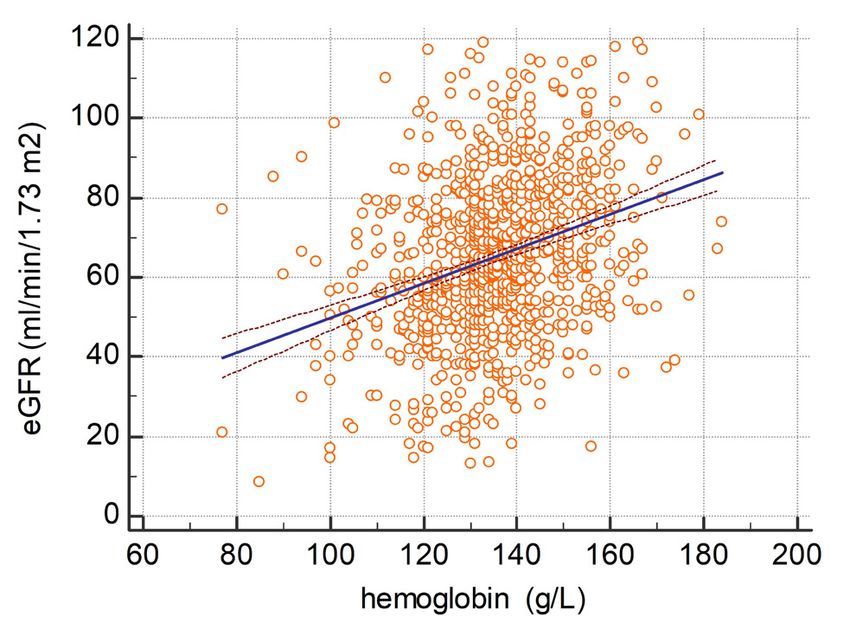

Bazdaric K, Sverko D, Salaric I, Martinović A, Lucijanic M. The ABC of linear regression analysis: What every author and editor should
know. European Science Editing 2021;47. DOI: 10.3897/ese.2021.e63780

Figure 2: A) Histogram of distribution of residuals of linear regression investigating estimated glomerular filtration rate (eGFR) and
haemoglobin relationship and B) scatter plot of residuals and haemoglobin values.

   The output of the program is shown in Figure 3. First, we should look at the P value to ensure that the model fits (number 1
in Figure 3). In our example, the P value for the overall model was 0.05, the regression is usually not interpreted. The next step is to
look for the coefficient of determination (R²) (number 2 in Figure 3). The closer the value of the coefficient to 1, the better the
prediction. In our example, R2 was 0.099, which enabled us to simply calculate the percentage of explained variation by multiplying
the proportion with 100; therefore, 0.099 × 100 = 9.9%, which is the proportion of the variation in eGFR that can be explained by
the haemoglobin value. Individual values of eGFR can then be predicted with the regression equation. In Figure 3, the regression
equation is formed by using regression coefficients (number 3 in Figure 3). The regression coefficient represents the amount of
change in the dependent variable per unit increase in the predictor variable. For example, if a patient has a haemoglobin level
of 130 g/L, the eGFR can be calculated as follows: eGFR = 6.556 + 0.433 × 130 = 62.8. Note that the regression line with a 95%
confidence interval is narrower in the middle and wider at the ends of data set, which means that the estimations are close to the
actual values had they been measured and can be interpreted with more confidence if the input data correspond to the average
values used in the study. Using values outside the range used in the study is called extrapolation and can yield unrealistic estimates
and therefore should be avoided.

Figure 3. Output of ‘multiple’ (but actually simple) linear regression provided by MedCalc, a statistical program.

                                                                 3 of 9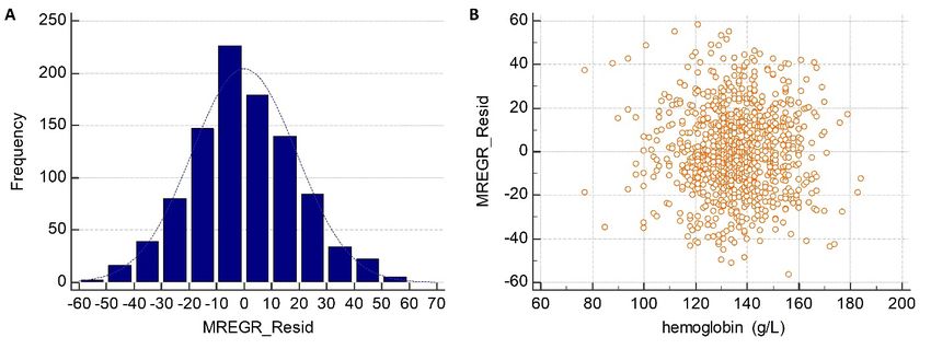

Bazdaric K, Sverko D, Salaric I, Martinović A, Lucijanic M. The ABC of linear regression analysis: What every author and editor should
know. European Science Editing 2021;47. DOI: 10.3897/ese.2021.e63780

Multiple regression analysis
Multiple linear regression is a statistical method similar to linear regression, the difference being that a multiple linear regression
uses more than one predictor or variable.4,5
   When building a model, the investigator has to be aware of the assumptions behind multiple regression analysis.
Assumptions in multiple regression analysis
Multiple regression analysis is a parametrical statistical method: it requires that the dependent variable be numerical (continuous)
on an interval or ratio scale, that the relationship between variables be linear, and that some other assumptions also be satisfied
(Table 1).9,10 The linearity is usually checked by correlating the variables using Pearson product moment correlation coefficient
and looking at the scatter plot.11–13 However, the linearity could be even better estimated by looking at the graph of residuals.10
Normality and homoscedasticity presume identical and independent distribution of residuals with a zero mean and constant
variance. The residual plot against the independent variable should show a random pattern (equally scattered and not forming
a U-shaped curve) and the variability of residuals should be relatively constant across all values of the independent variable.
Also, the residuals should be approximately normally distributed.11 Formal statistical testing of distribution normality is more
likely to yield significant results implying non-normal distribution in a large data set (as all statistical tests in large data sets
tend to do), automatically invalidating the assumptions behind the analysis. It is thus acceptable to check the histograms of
distribution of independent variables and residuals visually to ascertain whether we are dealing with unimodal and not highly
skewed distributions (especially if dealing with larger data sets comprising, for example, a few hundred or more cases). With
large samples, the requirement for normal distribution of residuals is less stringent because of the central limit theorem. Also,
assumptions for multiple regression are not met if any two variables are highly correlated, that is the condition of multicolinearity
is not satisfied.
    Regarding the required sample size, when choosing a number of independent variables, keep in mind that a minimum of 10
(or even up to 20) subjects are needed for each variable.11 Therefore, if a criterion is explained by three predictors, at least 30–60
subjects should be included (a free A-priori sample size calculator for multiple regression available at https://www.danielsoper.
com/statcalc/calculator.aspx?id=1).11

Table 1. Assumptions of multiple regression analysis

 Assumption                                    Assumption met if
 Dependent variable (criterion)                Dependent variable has to be on a continuous, interval, or ratio scale.
 Independent variables (predictors)            Multiple regression presumes including more than two independent variables as
                                               predictors. Predictors are mostly continuous, dichotomous, or binary variables (coded
                                               with ‘0’ and ‘1’).
 Linearity, normality, and homoscedasticity    For checking linearity, normality, and homoscedascity, use a residuals plot. Residuals
                                               have to be distributed with a zero mean and constant variance.
 Multicollinearity                             Only those predictors that are not highly correlated are to be included in the analysis.
 Number of predictors                          The number of predictors included in the analysis is dependent on the sample size.
                                               Online tools are available to ascertain the minimum sample size required.

Multiple linear regression
The formula for multiple regression is similar to that for simple linear regression; moreover, the value of the criterion is a linear
combination of predictors. The formula for multiple linear regression is as follows:
Y’ = B1X1 + B2X2 + ... + BnXn + A
where Y’ is the criterion, X1 to Xn are the predictor scores (X1, score of the first variable; X2, score of the second; etc.), B1 to Bn are
regression coefficients (similar to the slope in simple regression), and A is the intercept. 1
   Each predictor has its own weight that depends on the size of the regression coefficient (B) or standardized standardized beta
(β) coefficients.4,14 The regression coefficient represents the amount of change in the dependent variable for each unit increase in
the predictor variable.11,14 The result of a multiple regression is the optimal prediction of the criterion from two or more continuous
(or dichotomous or binary) predictors. The coefficient of multiple correlation ‘R’ is the correlation of all predictors with the
criterion, whereas the coefficient of multiple determination ‘R²’ describes the proportion of variance explained by predictors
varying from 0 to 1 (0% to 100%). The closer the value to 1, the better the prediction. 1,5,14
   Contributions of the independent variables to predict the criterion can be interpreted by using the multiple correlation
coefficient and standardized beta (β) coefficients. The contribution of a predictor (effect size of a variable) has to be presented with
a standardized β coefficient to be comparable between variables. B coefficients that are routinely obtained by MedCalc are not
standardized and are scale dependent and therefore unsuitable for this purpose. To obtain standardized β coefficients in MedCalc,
you need to standardize input data first in MS Excel. Despite the name, you do not standardize the coefficients after the analysis is
done; you standardize input variables by subtracting the mean from every observation and dividing it by the standard deviation

                                                                   4 of 9

Bazdaric K, Sverko D, Salaric I, Martinović A, Lucijanic M. The ABC of linear regression analysis: What every author and editor should
know. European Science Editing 2021;47. DOI: 10.3897/ese.2021.e63780

and thus obtain standardized variables with a mean of 0 and standard deviation of 1. To calculate the individual contribution of
a variable as a percentage, we use squared semi-partial coefficients of correlation (sr²), which are provided by MedCalc. Semi-
partial r² provides information on what proportion of the criterion variable can be explained with this particular predictor while
the rest of the correlations are excluded.
    To continue with the example with regard to predicting renal function quality in the multivariable context. In addition to
haemoglobin, we included in the model other clinical variables with potential associations with eGFR, such as body mass index,
left ventricle ejection fraction, age, and presence of coronary artery disease. All these parameters can either reflect on renal
function, be affected by it, or share some common risk factors and pathophysiologic mechanisms—we cannot judge causal
relationships between investigated variables; we can only assess whether significant relationships exist. The variable eGFR is the
criterion, whereas the other variables are considered predictors and entered as independent variables into the statistical program.
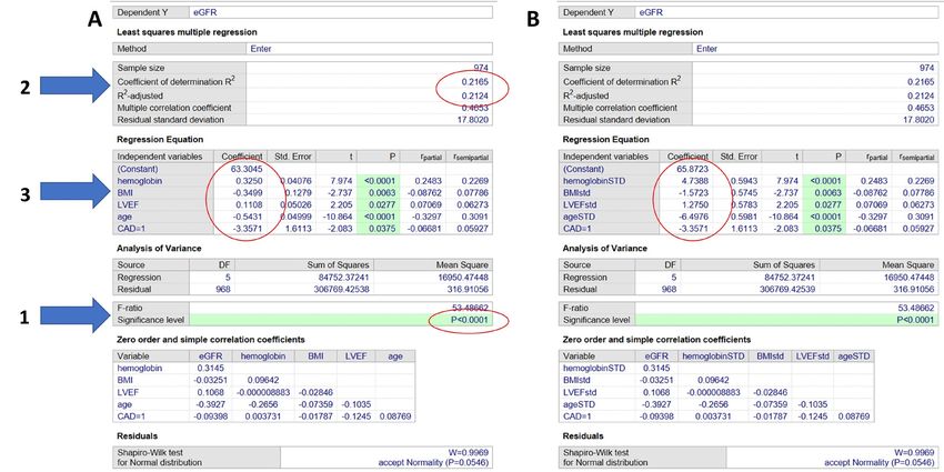
The program output is shown in Figure 4 and, as explained in the text below, two outputs are given: one with existing data set
(Figure 4A) and one with standardized input data (Figure 4B). The non-standardized data allow us to calculate eGFR from raw
data, whereas standardized data allow us to compare effect sizes.
    The residuals in the above example were normally distributed, suggesting that the assumptions were met. Also, a correlation
matrix between continuous variables is part of the program output (Figure 4) and helps us to understand the level of mutual
correlations that exist between used predictors, that is to assess multicolinearity. We were unable to put all the variables into a linear
correlation (presence of coronary artery disease (CAD = 1) is a binary variable and has to be coded in the program as ‘0’ if absent
and ‘1’ if present) and some of the investigated variables had low coefficients of correlation, implying that a linear relationship
actually does not exist (correlation coefficients between eGFR and body mass index and between eGFR and left ventricle ejection).
However, there are scientifically plausible reasons to include those variables into the analysis, so we decided to keep them.
    As in simple linear regression, first you have to check if the model fits (number 1 in Figure 4). Because the overall P value for the
regression is significant, we can proceed with interpreting the results. The second step is to look at the coefficient of determination
(R², number 2 in Figure 4). In our example, R² is 0.217, meaning that 21.7% of the eGFR is explained with this model. Because
this coefficient increases with the number of variables included in the model, it is advisable to present the adjusted coefficient of
multiple determination (adjusted for the number of variables included in the model). R²adjusted was 0.212, that is 21.2% of the eGFR
is explained.
    We further considered which variables explain, or are associated with, eGFR. We can search for the answer to that question under
number 3 in Figure 4. As can be observed, all of the included variables had statistically significant independent relationships with
eGFR. We can speculate that these variables might have different independent biological mechanisms behind the mathematical
relationship. Thereby, all variables should probably be considered separately if we wish to understand eGFR in patients with
atrial fibrillation. Individual contributions of particular predictors differ in the standardized β coefficients (Figure 4B), and semi-
partial correlation coefficients (Figure 4A and 4B) provide the same output, because the data were not standardized for the first
analyses but were standardized for the second one. Age and haemoglobin seem to explain the highest proportion of the eGFR.
Furthermore, different directions of predictors with dependent variables are present, indicating that patients who experienced
higher haemoglobin and left ventricle ejection fraction were more likely to have higher eGFR (positive B and β coefficients),
whereas patients with higher body mass index, older patients, and those with coronary artery disease were more likely to have
lower eGFR (negative B and β coefficients). The variable CAD = 1 beta coefficient is the adjusted mean difference in eGFR between
the two groups, meaning that the group in which coronary artery disease was present had lower eGFR (−3.35 points, or 3.35%).
    From the data (number 3 in Figure 4A), we can construct a regression equation for predicting the eGFR from the given data.
For example, if we have a 65-year-old patient with atrial fibrillation but without coronary artery disease, with a haemoglobin
level of 130 g/L, a body mass index of 30, and left ventricle ejection fraction of 60%, the patient’s eGFR can be easily calculated as
follows: eGFR = 63.3045 + 0.325 × 130 − 0.3499 × 30 + 0.1108 × 60 − 0.5431 × 65 − 3.3571 × 0 = 66.4.
    One can consider the obtained adjusted R² to be modest, because our model explained only 21% of the eGFR variance.
However, that small percentage does not invalidate the observations, which may have important clinical repercussions and can
help in planning future studies on the topic. As shown, all the investigated variables seem to contribute independently to eGFR
prediction. We did not recognize or could not measure major predictors of eGFR that would result in higher R² (we deliberately
chose not to consider such parameters of renal excretion function as urea and creatinine, because that would have resulted in a
‘self-fulfilling prophecy’ of little real interpretation value). It was also possible that some variables have no statistical significance
if analysed in a multivariable context. Such variables either truly do not have independent predictive properties or our sample
might have been too small for such analysis. Anyhow, such variable can yet be considered in a model if its inclusion increases
the adjusted R² substantially. If the analysis is repeated with and without such additional predictor(s) and if the variable is not
considered as a mandatory adjustment, then it should probably be excluded from the equation.
    Further exploratory analyses investigating whether interactions between different independent variables and the dependent
variable exist can be undertaken to better understand the given data set. Interaction is present when the degree of association
between two variables changes depending on the value of the third one, that is when one variable moderates the relationship
between two other variables. The present article does not deal with this issue in more detail because the complexity of the theme
and the lack of space do not permit a more detailed discussion; however, we plan to do so in future.

                                                                  5 of 9

Bazdaric K, Sverko D, Salaric I, Martinović A, Lucijanic M. The ABC of linear regression analysis: What every author and editor should
know. European Science Editing 2021;47. DOI: 10.3897/ese.2021.e63780

std = standardized
Figure 4: Results of multiple regression using MedCalc. A) data as originally recorded and B) data standardized to obtain
standardized β coefficients. eGFR, estimated glomerular filtration rate; BMI, body mass index; LVEF, left ventricular ejection fraction;
CAD, coronary artery disease.

Some common areas of errors in presenting regression analysis
Adequate guidelines are available from the EQUATOR network for almost every type of article. These include guidelines for
reporting statistics, for example the ‘SAMPL Guidelines for Biomedical Journals’ written by Tom Lang and Doug Altman, which
also discuss the reporting of regression analysis in detail.15 We propose a quick checklist that can help authors and editors in
evaluating multiple regression analyses.

Table 2. A checklist for multiple regression analysis

 Question                                   Answer
 Does the title or main text use causal     The title of an article in which simple or multiple regression is used contains words such
 language appropriately?                    as ‘correlation’, ‘relation’ and ‘association’ but avoids words such as ‘influence’ or ‘cause’.
 Are statistical assumptions for multiple   See Table 1.
 regression satisfied?

 Are variable transformations used          Check whether the assumptions are met after carrying out a variable transformation:
 sensibly?                                  If the relationship between variables needs to be linear, a graph of the transformed
                                            variable should reflect that.
 Is the analysis significant?               If the analysis is not significant (P

Bazdaric K, Sverko D, Salaric I, Martinović A, Lucijanic M. The ABC of linear regression analysis: What every author and editor should
know. European Science Editing 2021;47. DOI: 10.3897/ese.2021.e63780

it is well described in the literature and it was not easy to understand before the discovery that secondary depletion of von
Willebrand factor (glicoprotein crucial for platelet adhesion to damaged sites in the vasculature) occurs because of the high
number of circulating platelets.17
    Therefore, the title of an article in which simple or multiple regression is used should contain words such as ‘correlation’, ‘relation’,
and ‘association’ but avoid words such as ‘influence’ or ‘cause’ because they imply, possibly incorrectly, a causal relationships
between variables.18,19 Some authors consider the term ‘correlation’ more appropriate than the term ‘association’ because the latter
is usually used for expressing the relationship between categorical variables.20 The distinction, however, is debatable. The terms
‘multivariate’ and ‘multivariable’ are often used: a multivariable model refers to an analysis with one dependent and two or more
(multiple) independent variables whereas a multivariate analysis refers to an analysis with more than one outcomes (for example
repeated measures) and multiple independent variables.21
    JAMA editors strongly suggest avoiding causal language except in randomized controlled trials (https://jamanetwork.com/
journals/jama/pages/instructions-for-authors#SecReportsofSurveyResearch). Furthermore, they also advise describing methods
and results using the words ‘association’ and ‘correlation’ and to avoid avoiding words that imply a ‘cause-and-effect’ relationship.
The same principle can be applied to studies where regression analysis is used as a statistical method.

Area 2: Assumptions for calculating multiple regression
A long time ago, the medical editor and writer Tom Lang wrote that “every scientific article that includes statistical analysis
should contain a sentence confirming that the assumptions on which the analysis is based were met.”10 It is important to notice
that violating the assumptions (or ignoring them) makes the estimates obtained by regression analysis less reliable, possibly
unreliable, or even false. Real-life clinical data rarely meet all the assumptions that multiple regression requires. However, if
authors decide to use this method, it is fair to make attempts to limit the violations and to recognize the limitations of their work
so that readers (and editors) can judge the work objectively. Furthermore, other statistical analyses may be chosen instead, if the
main assumptions are not met.
   It should be noted that linearity cannot be checked for binary variables and that non-linearly correlated variables might be
significant predictors of the criterion of interest, as described in our example. Authors should be guided by logic and scientific
plausibility. If the relationship between the dependent and the independent variables is not linear, variables can be transformed,9
and authors are advised to consider categorizing the predictors if they believe there is a non-linear relationship to overcome
the breach of linearity. By transforming either the dependent or the independent variable we can obtain better coefficients of
determination and better linearity. Possible transformation options include creating an exponential model (testing different
logarithms of dependent variables), a quadratic model (taking the square root, the 3rd root, etc of an independent variable), a
reciprocal model (1/dependent variable), a logarithmic model (different logarithms of the independent variable), or a combination
of models (combining different types of transformations for both dependent and independent variables). We would like to point
out that a simple one-time transformation of the dependent variable (using logarithmic transformation, for example), without
assessing whether assumptions are improved by the process, does not make sense and does not suddenly make the regression
unbiased and acceptable. However, this is a phenomenon often encountered in medical journals because many authors consider
this to be a great move to checkmate the reviewers. If authors, editors, or reviewers realize that the assumptions have not been
met and therefore ask for solutions, other methods of regression can be suggested or other statistical methods can be used. In
such cases, a logistic regression (if authors wish to base their conclusions on the prediction that the dependent variable odds are
higher or lower than something else) or a Poisson regression (in dealing with numerical data that are usually highly skewed) can
be used for the same purpose and can yield similar conclusions. Authors can still insist on using a multiple regression and choose
to ignore the above-mentioned points; however, in that case, they are concerned mainly with describing their data set and not in
making inferential conclusions on the population in general.
   The point is not to include all measured variables in the model but only those clinically meaningful that fit well.5 It is a common
practice that it is appropriate to include variables in the multivariable model. It is recommended that recognized predictors
described in the literature be used, as well as variables that show significant univariate associations or that have clinically
meaningful biological relationships despite not being significantly related in the current data set. Furthermore, variables such as
age and sex can be considered mandatory adjustments if the sample size permits it. It is possible that the number of variables that
need to be considered is much higher than the possibilities afforded by sample size. In that case, the authors must consciously
limit their analyses or perform automatic stepwise model building, letting the computer chose the best predictors. However, this
does not absolve authors of the responsibility of interpreting how and why the variables in the final model were chosen.

Area 3: Significance of regression
A common and frequent mistake is to interpret regression models that are not significant. The results of regression can be
interpreted by the strength of the evidence: a small P value suggests stronger evidence for rejecting the null hypothesis. An
arbitrary value of P, namely 0.05, is very common in the literature, and P

Bazdaric K, Sverko D, Salaric I, Martinović A, Lucijanic M. The ABC of linear regression analysis: What every author and editor should
know. European Science Editing 2021;47. DOI: 10.3897/ese.2021.e63780

Area 4: Interpretation of regression: coefficient of determination ‘R2’ and beta coefficients
There are different models of regression and sometimes investigators or authors think that if they choose a bunch of variables,
at least some of them will eventually prove significant. The same applies to choosing a different approach to model building
(backward or forward stepwise regression), which can yield different results. This practice is called P-hacking and it is definitely
something to be avoided.22 The analysis could even be statistically significant because of the sample size or the number of variables
without having a real interpretation value.
    When using multiple regression to derive the prediction equation, to ensure that the regression is not only significant (P

Bazdaric K, Sverko D, Salaric I, Martinović A, Lucijanic M. The ABC of linear regression analysis: What every author and editor should
know. European Science Editing 2021;47. DOI: 10.3897/ese.2021.e63780

Acknowledgements
We thank Ivana Jurin and Irzal Hadzibegovic for making available the data set used for the examples of regression in this article.

Funding
None

Competing interests
Ksenija Bazdaric is the Editor in Chief of European Science Editing. The peer review process and the decision were led by other
editors.

References
1 Montgomery, Douglas C; Peck EAVGC. Introduction to Linear Regression Analysis. 5th ed. Wiley; 2012.
2 Udovičić M, Baždarić K, Bilić-Zulle L, Petrovečki M. What we need to know when calculating the coefficient of correlation? | Što treba znati kada
   izračunavamo koeficijent korelacije? Biochem Medica. 2007;17(1):10-15.
3 Lang TA, Altman DG. Basic statistical reporting for articles published in Biomedical Journals: The “Statistical analyses and methods in the published
   literature” or the SAMPL guidelines. Int J Nurs Stud. 2015;52(1):5-9. doi:10.1016/j.ijnurstu.2014.09.006
4 Tabachnick, Barbara G; Fidell LS. Using Multivariate Statistics. Pearson Education Ltd; 2013.
5 Triola MM; Triola MF. Correlation and Regression. In: Biostatistics for the Biological and Health Sciences with Statdisk. Pearson Education Ltd; 2014:426-488.
6 Jurin I, Lucijanic M, Jurin H, et al. Patients with atrial fibrillation and mid-range ejection fraction differ in anticoagulation pattern, thrombotic and mortality
    risk independently of CHA(2)DS(2)-VAS(C) score. Heart Vessels. 2020;35(9):1243-1249. doi:10.1007/s00380-020-01603-2
7 Levey AS, Bosch JP, Lewis JB, Greene T, Rogers N, Roth D. A more accurate method to estimate glomerular filtration rate from serum
   creatinine: a new prediction equation. Modification of Diet in Renal Disease Study Group. Ann Intern Med. 1999;130(6):461-470.
   doi:10.7326/0003-4819-130-6-199903160-00002
8 Lane DM. Prediction. In: HyperStat Online Statistics Textbook. ; 2013. http://davidmlane.com/hyperstat/prediction.html
9 Ingelfinger JA. Biostatistics in Clinical Medicine. Vol 347.; 1994. doi:10.1016/0197-2456(85)90099-6
10 Lang T. Twenty statistical errors even you can find in biomedical research articles. Croat Med J. 2004;45(4):361-370.
11 Hill, T. & Lewicki P. How To Find Relationship Between Variables, Multiple Regression. Electronic Statistics Textbook. Published 2007. http://www.statsoft.
   com/Textbook/Multiple-Regression
12 Petrie A, Sabin C. Medical Statistics at a Glace. 3rd ed. Wiley; 2017. doi:10.1093/ije/30.2.407
13 Hrabač P, Trkulja V. Of cheese and bedsheets - some notes on correlation. Croat Med J. 2020;61(3):293-295. doi:10.3325/cmj.2020.61.293
14 Fox J. Applied Regression Analysis & Generalized Linear Models. 3rd ed. SAGE Publications; 2016.
15 Altman DG, Gore SM, Gardner MJ, Pocock SJ. Statistical guidelines for contributors to medical journals. 1983;286(May):1489-1493.
16 Wager E. Getting Research Published. 3rd ed. CRC Press; 2016.
17 Van Genderen PJJ, Leenknegt H, Michiels JJ, Budde U. Acquired von willebrand disease in myeloproliferative disorders. Leuk Lymphoma. 1996;22(SUPPL.
   1):79-82. doi:10.3109/10428199609074364
18 Assel M, Sjoberg D, Elders A, et al. Guidelines for reporting of statistics for clinical research in urology. 2019;(5):401-410. doi:10.1111/bju.14640
19 Thapa DK, Visentin DC, Hunt GE, Watson R, Cleary M. Being honest with causal language in writing for publication. J Adv Nurs. 2020;76(6):1285-1288.
   doi:10.1111/jan.14311
20 Lang, TA; Secic M. How to Report Statistics in Medicine. 2nd ed. American College of Physicians; 2006.
21 Ebrahimi M, Ms K, Ms RJ, Ms EZ. Letter Distinction Between Two Statistical Terms : Multivariable and Multivariate Logistic Regression. 2020;2020:1-2.
   doi:10.1093/ntr/ntaa055
22 Nuijten MB. Preventing statistical errors in scientific journals. Eur Sci Ed. 2016;42(1):8-10.
23 Marsh J. Should editors be more involved in the development of reporting guidelines? Eur Sci Ed. 2018;44(1):2-3. doi:10.20316/ESE.2018.44.17024

                                                                                9 of 9