OUTPACE long duration stations: physical variability, context of biogeochemical sampling, and evaluation of sampling strategy - Biogeosciences
←
→
Page content transcription
If your browser does not render page correctly, please read the page content below
Biogeosciences, 15, 2125–2147, 2018
https://doi.org/10.5194/bg-15-2125-2018
© Author(s) 2018. This work is distributed under
the Creative Commons Attribution 4.0 License.

OUTPACE long duration stations: physical variability, context of
biogeochemical sampling, and evaluation of sampling strategy
Alain de Verneil1,a , Louise Rousselet1 , Andrea M. Doglioli1 , Anne A. Petrenko1 , Christophe Maes2 ,
Pascale Bouruet-Aubertot3 , and Thierry Moutin1
1 Aix Marseille Univ., Université de Toulon, CNRS, IRD, MIO UM 110, 13288, Marseille, France
2 Universitéde Bretagne Occidentale (UBO), Ifremer, CNRS, IRD, Laboratoire d’Océanographie Physique et Spatiale
(LOPS), IUEM, 29280, Brest, France
3 Sorbonne Université (UPMC, Univ Paris 06)-CNRS-IRD-MNHN, LOCEAN, Paris, France
a now at: The Center for Prototype Climate Modeling, New York University in Abu Dhabi, Abu Dhabi, UAE

Correspondence: Alain de Verneil (ajd11@nyu.edu)

Received: 26 October 2017 – Discussion started: 2 November 2017
Revised: 14 March 2018 – Accepted: 15 March 2018 – Published: 10 April 2018

Abstract. Research cruises to quantify biogeochemical             analyses presented here to verify the appropriate use of the
fluxes in the ocean require taking measurements at stations       drifter platform.
lasting at least several days. A popular experimental design
is the quasi-Lagrangian drifter, often mounted with in situ
incubations or sediment traps that follow the flow of water
over time. After initial drifter deployment, the ship tracks      1   Introduction
the drifter for continuing measurements that are supposed to
represent the same water environment. An outstanding ques-        Biogeochemical cycles dictate the global distribution and
tion is how to best determine whether this is true. During        fluxes of the chemical elements. Quantifying the mechanisms
the Oligotrophy to UlTra-oligotrophy PACific Experiment           that mediate the various forms key elements take in these cy-
(OUTPACE) cruise, from 18 February to 3 April 2015 in             cles, especially in the midst of ongoing climate change in the
the western tropical South Pacific, three separate stations of    ocean, is vital to understanding the future evolution of the
long duration (five days) over the upper 500 m were con-          Earth system (Falkowski et al., 2000; Davidson and Janssens,
ducted in this quasi-Lagrangian sampling scheme. Here we          2006; Gruber and Galloway, 2008). Considering the wide
present physical data to provide context for these three sta-     diversity of environments where biogeochemical processes
tions and to assess whether the sampling strategy worked,         take place, it is not surprising that each sub-discipline has
i.e., that a single body of water was sampled. After analyz-      its own challenges with regards to collecting and processing
ing tracer variability and local water circulation at each sta-   samples. The sampling protocols put in place thus need to
tion, we identify water layers and times where the drifter        ensure the mechanisms of interest are isolated and put into
risks encountering another body of water. While almost no         their proper context.
realization of this sampling scheme will be truly Lagrangian,        In the world’s surface oceans, a dominant difficulty is the
due to the presence of vertical shear, the depth-resolved ob-     medium itself: water. Sampling in a fluid that is always li-
servations during the three stations show most layers sam-        able to move normally requires that one of two approaches be
pled sufficiently homogeneous physical environments dur-          taken. In the first approach, a geographic location is chosen
ing OUTPACE. By directly addressing the concerns raised           and then repeatedly sampled. This produces an Eulerian per-
by these quasi-Lagrangian sampling platforms, a protocol of       spective, and this methodology is employed by definition at
best practices can begin to be formulated so that future re-      permanent mooring platforms. Set geographic locations are
search campaigns include the complementary datasets and           also often used to define time series or recurrent sampling
                                                                  locations, for example stations ALOHA, BATS, CalCOFI,

Published by Copernicus Publications on behalf of the European Geosciences Union.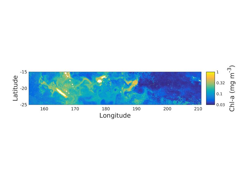
2126                                                                                       A. de Verneil et al.: LD OUTPACE

DYFAMED, and PAPA (Karl and Lukas, 1996; Schroeder                 time over great distances. Therefore, before deployment the
and Stommel, 1969; Steinberg et al., 2001; Bograd et al.,          selection of sampling sites needs to be carefully considered.
2003; Marty et al., 2002; Freeland, 2007). These sites can         Unless the focus of study, fronts and filaments need to be
be combined into worldwide networks and initiatives such as        avoided because shearing will quickly separate water parcels
OceanSITES (Send et al., 2010). While this strategy makes          at different depths in the direction of the structure’s align-
no attempt to actually follow a given water parcel, if cur-        ment; finding signs of their presence has become more feasi-
rents are relatively weak during a single field campaign then      ble with satellite data. An eddy can be targeted because of its
the variability due to advection can be ignored. Unfortu-          coherence, and there are ways to confirm that sampling is in-
nately, the spatio-temporal scales of shipboard station sam-       deed inside of it (Moutin and Prieur, 2012). In other words,
pling (in time, days to weeks; in space, 1–100 km) overlap         if a physical structure is targeted or identified, its particu-
with a multitude of physical phenomena ubiquitously found          lar nature supersedes other considerations. These structures
in the ocean, ranging from internal waves, submesoscale tur-       are not necessarily representative of the World Ocean, and
bulence, up to mesoscale eddies (d’Ovidio et al., 2015). All       so many biogeochemical measurements will be taken else-
of these motions can easily transport water such that instan-      where. For the campaigns where sites are far (possibly by
taneously observed temperature, salinity, and by extension         design) from obvious, organized mesoscale structures, there
the organisms and chemical environments mediating biogeo-          is still a need to conduct an independent, post-cruise valida-
chemical processes, are markedly different from some mean          tion of the drifter’s success, which is the focus of the present
value or state.                                                    study.
   One way to rectify physical displacements is the sec-              Before proceeding into the description of our methodol-
ond sampling approach, namely to follow the water during           ogy, a few remarks are needed regarding its applicability.
ongoing experiments. This approach creates a Lagrangian            We already mentioned that we will consider regions away
point of view. A common implementation of this strategy            from strong, organized mesoscale structure. Additionally, the
is with quasi-Lagrangian drifting moorings (Landry et al.,         method relies upon independent physical, not biogeochemi-
2009; Moutin et al., 2012). These drifters are structured so       cal, measurements to indicate a change of water mass due to
that a vertical line with sampling devices (e.g., incubation       the drifter not being Lagrangian. This approach does not de-
bottles and/or sediment traps) drifts along with the flow.         tect the existence of biogeochemical gradients in water that
This approach has been in routine use for decades across           might exist on smaller scales, so application of our method
the globe; some examples of French campaigns known to              requires the user to apply contextual knowledge of their sam-
the authors include the OLIPAC (1994), PROSOPE (1999),             pling region and keep this possibility in mind. For this study,
BIOSOPE (2004), and BOUM (2008) experiments (all data              a regional biogeochemical gradient was expected (Moutin
and metadata accessible from the LEFE CYBER website,               et al., 2017) and rationales for this method’s application will
http://www.obs-vlfr.fr/proof/cruises.php, last access: 6 April     be provided.
2018).                                                                The Oligotrophy to UlTra-oligotrophy PACific Experi-
   Naturally, the question arises whether the trajectory un-       ment (OUTPACE) cruise provided an opportunity to assess
dertaken by the drifting mooring in the quasi-Lagrangian ap-       the success of the quasi-Lagrangian sampling strategy. Con-
proach accurately represents the water movements at each of        ducted from 18 February to 3 April 2015 in the western trop-
the sampling sites. If the drifter is successful in following      ical South Pacific (WTSP), one of the goals of OUTPACE
the water, then indeed a single biogeochemical setting will        was to assess the regional contribution of nitrogen fixation
have been sampled; if it is not successful, then the risk grows    as a biogeochemical process to the biological carbon pump
that a different environment has been brought in via advec-        (Moutin et al., 2017). During the cruise, three long duration
tion. Previous efforts by physicists to make floats Lagrangian     (LD) stations employed the quasi-Lagrangian strategy. In the
show the effort needed to make an instrument neutrally buoy-       subsequent discourse regarding these stations, we proceed as
ant, and these floats have been instrumental in demonstrating      follows. Section 2 describes how the drifting mooring was
complicated flow regimes (D’saro et al., 2011). In contrast,       deployed, our methodological strategy, how concurrent data
the quasi-Lagrangian platform, with a variable distribution        were collected, and the analyses undertaken to answer our
of incubation bottles, will necessarily fail to be Lagrangian      central question of whether we sampled a single environ-
in finite time outside of a barotropic flow where currents are     ment. We then present the data and results in Sect. 3, fol-
the same throughout the water column. As a result, ensuring        lowed by a discussion in Sect. 4. The paper finishes in Sect. 5
the success of this strategy requires taking into account how      with a summary of our recommendations regarding future
different currents potentially shorten the timespan of validity.   implementations of this sampling strategy.
In fast-moving flows with strong vertical shear and possible
vertical motions, such as zones of enhanced mesoscale tur-
bulence near fronts and filaments, the drifter will not be La-
grangian for long. Alternatively, if a drifter is trapped inside
a coherent eddy, it can follow a similar water mass for a long

Biogeosciences, 15, 2125–2147, 2018                                                     www.biogeosciences.net/15/2125/2018/
A. de Verneil et al.: LD OUTPACE 2127
(a)
Chl a (mg m-3)
Latitude(°N)
-15 1
LDA LDB
0.32
-20
LDC 0.1
-25 0.03
(b) 160 170 180 190 200 210
Latitude(°N)
-15 31
SST (°C)
29
-20
27
-25 25
160 170 180 190 200 210
Longitude (° E)
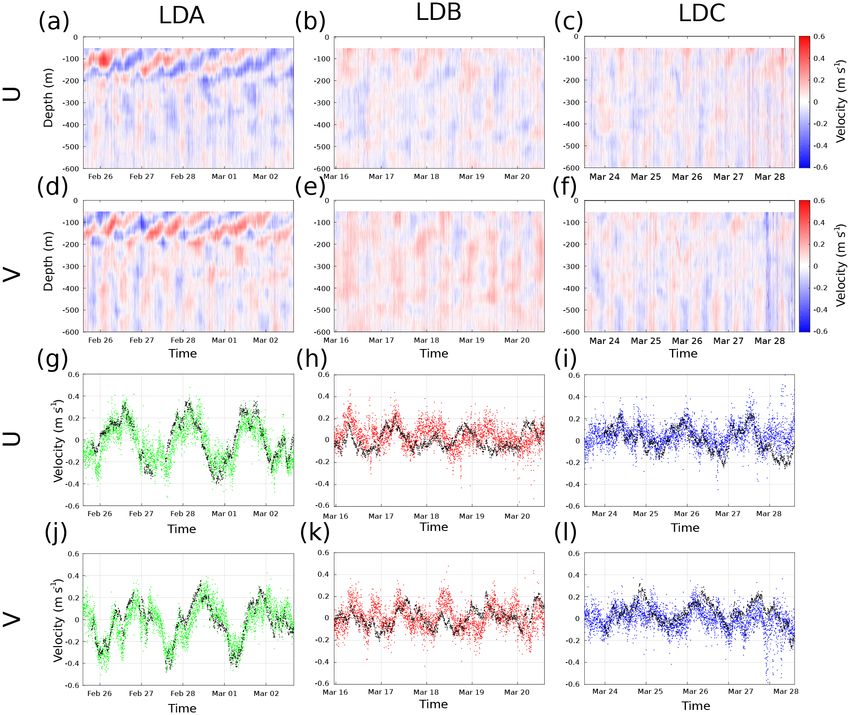
Figure 1. Satellite surface (a) chl a and (b) SST for the OUTPACE cruise. Pixel data are weighted by the normalized inverse distance squared
between each pixel and the RV L’Atalante’s daily position over the 42 days of OUTPACE. Ship track shown in white. LD station locations
shown with black +’s. Domains used in Fig. 2 are shown by color-coded rectangles, with green for LDA, red for LDB, and blue for LDC.
2 Materials and methods jacent to the site. The number of drifters deployed are sum-
marized in Table 1, and their mean initial positions were 1.1,
In this section, we begin by describing the general manner 1.6, and 0.9 km away from the first CTD of station LDA,
in which the three LD stations were conducted during the LDB, and LDC, respectively. At the start of each station,
OUTPACE cruise. Following an outline of the methodolog- two quasi-Lagrangian drifting moorings were deployed dur-
ical strategy, we present the different data sources and their ing the OUTPACE LD stations with surface floats. The first
processing. Additionally, we describe in detail the analyses drifting mooring, hereafter referred to as the SedTrap Drifter,
needed to answer our central question regarding sampling in had a “holey sock” attached at 15 m depth. It was followed
a coherent environment. actively by the ship and is the emphasis of this study. It
had three sediment traps (Technicap PPS5/4) fixed at 150,
2.1 Sampling strategy 250, and 500 m depth, along with onboard conductivity–
temperature–depth (CTD) sensors and current meters, de-
The OUTPACE cruise occurred aboard the RV L’Atalante scribed below in Sect. 2.4.1 and 2.6, respectively. The Sed-
from 18 February to 3 April in late austral summer, start- Trap Drifter was deployed at the beginning of each sta-
ing in New Caledonia and finishing in Tahiti, traveling over tion and was left in the water until the station’s completion.
4000 km. Stations were conducted in a mostly zonal tran- The second drifting mooring, referred to as the production
sect traveling west to east, with the ship track averaging line, housed in situ incubation platforms for measuring pri-
near 19◦ S. The three LD stations, denoted as LDA, LDB, mary production, nitrogen fixation, oxygen, and other bio-
and LDC, and lasting 5 days each, were designed to resolve geochemical measurements (see Moutin and Bonnet, 2015,
a regional zonal gradient in oligotrophy, the existence of for more documentation). The production line was rede-
which is reflected in the surface chlorophyll a (chl a) data ployed on a daily basis close to the SedTrap Drifter. While
(Fig. 1a). As described in the introductory article of this spe- no telemetry exists for the production line, the CTD casts
cial issue (Moutin et al., 2017), site selection for the LD from which incubation water was drawn ranged from 300 m
stations involved identifying physical structures by use of to 5.7 km from the SedTrap drifter. After 5 days, the SedTrap
the SPASSO software package (http://www.mio.univ-amu. Drifter was recovered, and the LD station completed. Occa-
fr/SPASSO/, last access: 6 April 2018) using near real- sions when the exact implementation of this general strategy
time satellite imagery, altimetry, and Lagrangian diagnostics was not realized will be mentioned in following sections for
(Doglioli et al., 2013; d’Ovidio et al., 2015; Petrenko et al., the relevant measurements. A summary of time duration for
2017). each data source can be found in Table 1.
Before starting each LD station, surface velocity program
(SVP; Lumpkin and Pazos, 2007) drifters were deployed ad-
www.biogeosciences.net/15/2125/2018/ Biogeosciences, 15, 2125–2147, 2018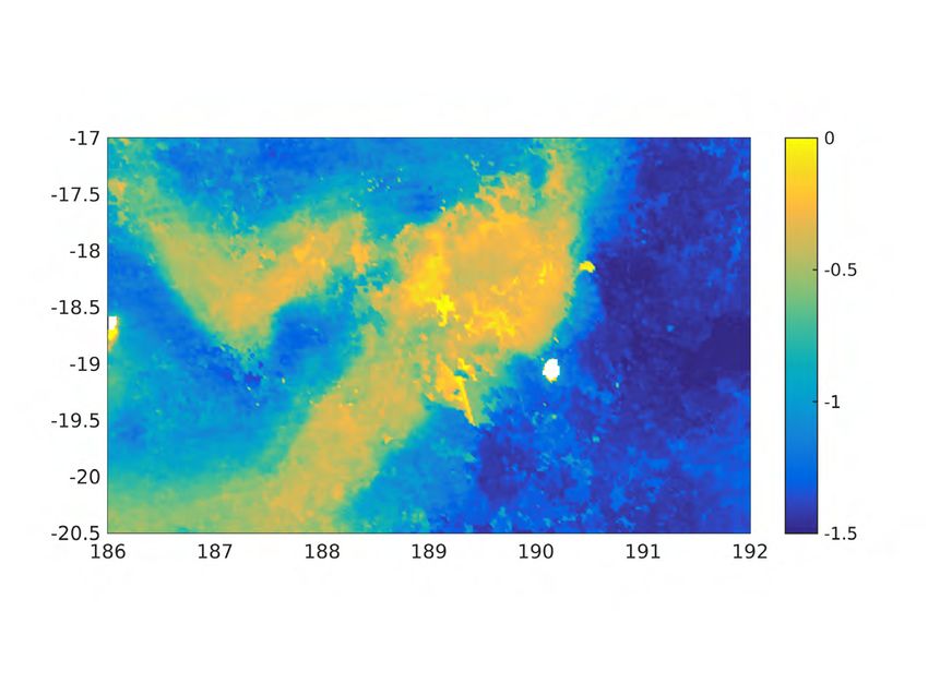
2128                                                                                            A. de Verneil et al.: LD OUTPACE

Table 1. Start and stop times for the time series data in each LD station of OUTPACE. Times expressed in DD/MM/YYYY HH:MM:SS
(GMT) format. When multiple instruments were deployed or multiple discrete observations made, this is also noted.

                 STATION
                 LDA           Instrument    CTD rosette               SVP                      AQUADOPP
                 (19.21◦ S,    Number        46 casts                  3 drifters               6 deployed
                 164.69◦ E)    Start         25/02/2015 14:09:18       25/02/2015 20:00:00      26/02/2015 22:40:00
                               Stop          02/03/2015 16:10:10       02/03/2015 22:00:00      02/03/2015 16:10:00
                               Duration      5 days 2 h 0 min 52 s     5 days 2 h               3 days 17 h 30 min
                               Instrument    SADCP 150                 SADCP 38                 SedTrap position
                               Start         25/02/2015 14:09:57       25/02/2015 14:10:26      25/02/2015 19:01:13
                               Stop          02/03/2015 16:09:51       02/03/2015 16:08:38      02/03/2015 22:00:00
                               Duration      5 days 1 h 59 min 54 s    5 days 1 h 58 min 12 s   5 days 2 h 58 min 47 s
                 LDB           Instrument    CTD rosette               SVP                      AQUADOPP
                 (18.24◦ S,    Number        47 casts                  6 drifters               6 deployed
                 189.14◦ E)    Start         15/03/2015 12:04:44       15/03/2015 10:00:00      15/03/2015 23:10:00
                               Stop          20/03/2015 14:16:13       20/03/2015 23:00:00      20/03/2015 14:15:00
                               Duration      5 days 2 h 11 min 29 s    5 days 13 h              4 days 15 h 5 min
                               Instrument    SADCP 150                 SADCP 38                 SedTrap position
                               Start         16/03/2015 08:51:53       15/03/2015 23:06:31      15/03/2015 12:15:48
                               Stop          20/03/2015 14:15:54       20/03/2015 14:14:50      20/03/2015 21:00:00
                               Duration      4 days 5 h 24 min 1 s     4 days 15 h 8 min 19 s   5 days 8 h 44 min 12 s
                 LDC           Instrument    CTD rosette               SVP                      AQUADOPP
                 (18.42◦ S,    Number        46 casts                  4 drifters               6 deployed
                 194.06◦ E)    Start         23/03/2015 23:10:57       23/03/2015 12:00:00      23/03/2015 23:25:00
                               Stop          28/03/2015 14:32:30       28/03/2015 22:00:00      28/03/2015 14:30:00
                               Duration      4 days 15 h 21 min 33 s   5 days 10 h              4 days 15 h 5 min
                               Instrument    SADCP 150                 SADCP 38                 SedTrap position
                               Start         23/03/2015 12:08:12       23/03/2015 12:06:55      23/03/2015 12:19:55
                               Stop          28/03/2015 14:30:31       28/03/2015 14:31:39      26/03/2015 03:31:34
                               Duration      5 days 2 h 22 min 19 s    5 days 2 h 24 min 44 s   2 days 15 h 11 min 39 s

   Between the LD stations, 15 short duration (SD) stations            2.2   Post-validation method
lasting approximately 8 h each were interspersed along the
ship’s trajectory in roughly equidistant sections (Fig. 1b).           The goal of this study is to evaluate whether the three LD sta-
Among the measurements made, CTD casts from SD sta-                    tions sampled in a homogeneous body of water during OUT-
tions will figure into the validation process in this study. Most      PACE. In order to achieve this goal, a number of steps were
casts (both LD and SD) were at least 200 m, with at least one          undertaken:
2000 m cast for all stations. These casts were conducted with
                                                                         – Validity of application and environmental context. As
the same CTD rosette platform described more fully below
                                                                           mentioned in the introduction, if a physical structure
in Sect. 2.3.1.
                                                                           such as an eddy or front is present, its dynamics will
   Throughout the cruise, surface conductivity–temperature
                                                                           dominate and must be taken into account. Additionally,
measurements from the thermosalinograph (TSG) and cur-
                                                                           since we used physical water properties in this study,
rents from shipboard acoustic Doppler current profilers
                                                                           we must determine whether biogeochemical gradients
(SADCP) were collected. Their processing is described in
                                                                           existed at smaller scales. For this purpose, we looked at
Sect. 2.4.1 and 2.6, respectively.
                                                                           remote sensing data.

                                                                         – Establishment of statistical baseline. To evaluate
                                                                           whether station sampling remained in one water mass,
                                                                           the water mass itself needed to characterized. This was

Biogeosciences, 15, 2125–2147, 2018                                                          www.biogeosciences.net/15/2125/2018/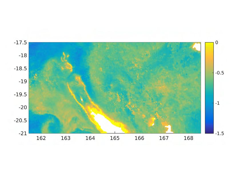
A. de Verneil et al.: LD OUTPACE                                                                                            2129

      achieved by initializing a baseline within the time se-     in SST and chl a distributions indicated strong surface forc-
      ries of hydrographic properties. The subsequent time        ing or the passage of gradients, which could invalidate the
      evolution of these properties within the defining dataset   applicability of the method.
      served as a first test for whether sampling stayed in one      Local surface currents derived from altimetry were also
      environment.                                                provided by CLS with support from CNES. These data come
                                                                  from the Jason-2, Saral-AltiKa, Cryosat-2, and HY-2A mis-
  – Spatial scale determination and baseline context. If          sions, cover a domain from 140 to 220◦ E, and 30◦ S to
    time series analysis showed no change in water proper-        the Equator, covering the yearlong period of June 2014 to
    ties, complementary data from farther away were com-          May 2015. The velocity grid had a 1/8◦ resolution, applying
    piled to evaluate the spatial scale at which the water        the FES2014 tidal model and CNES_CLS_2015 mean sea
    mass did change. These data were also used to contex-         surface. Ekman effects due to wind were also added using
    tualize whether the statistical baseline over-estimated or    ECMWF ERA INTERIM model output.
    under-estimated water mass variability.
                                                                  2.4     Establishment of statistical baseline
  – Currents analysis and Lagrangian risk. The spatial
    scale of the water mass already determined, water tra-
                                                                  Water mass characterization depended upon observations of
    jectories were used to evaluate at what point the ob-
                                                                  conservative temperature (CT ) and absolute salinity (SA ), or
    served flow regime might have brought another water
                                                                  T -S measurements. The statistical baseline, which served as
    mass into contact with LD station sampling near the
                                                                  the reference for each LD station, needed to reflect the initial
    SedTrap drifter.
                                                                  state of the water near the SedTrap drifter. While the SedTrap
The following sections in the methods are organized around        drifter itself had CTD sensors onboard, these were fixed in
these steps, detailing the data and analyses involved for each    depth and did not resolve the full variability of the water col-
step.                                                             umn. Additionally, although the SedTrap drifter served as the
                                                                  moving station’s location, water derived from the shipboard
2.3   Validity of method application and environmental            CTD rosette ultimately served as the source material for the
      context                                                     biogeochemical measurements taken during the cruise. The
                                                                  shipboard casts were always positioned near the SedTrap
Detection of physical structures and biogeochemical gradi-        drifter, averaging 1.2 km over the entire cruise. For these rea-
ents used satellite measurements of sea surface temperature       sons the CTD cast data were chosen for the baseline calcu-
(SST), surface chl a, and sea surface height with its asso-       lation, while both SedTrap drifter and CTD cast data were
ciated geostrophic currents. These data were also used in         included in the time series analysis.
the LD site selection phase (Sect. 2.1). All processed satel-
lite data were provided by CLS with support from CNES.            2.4.1    CTD data for time series analysis
SST was derived from a combination of AQUA/MODIS,
TERRA/MODIS, METOP-A/AVHRR, METOP-B/AVHRR                         The shipboard CTD employed during OUTPACE was a
sensors, with the daily product produced being a weighted         Seabird SBE 9+ CTD rosette with two CTDs installed. Data
mean spanning 5 days (inclusive) previous to the date in          from each cast were calibrated and processed post-cruise us-
question. Weighting was greater for more recent data. Sim-        ing Sea-Bird Electronics software into 1 m bins. All CTD
ilar to SST, chl a was a 5 day weighted mean produced by          data from other instruments mentioned later were likewise
the Suomi/NPP/VIIRS sensor. The SST and chl a products            processed using Sea-Bird Electronics software. SA , CT , and
had a 0.02◦ resolution, equivalent to ∼ 2 km. These satellite     potential density (σθ ) were calculated using the TEOS-10
products spanned from 1 December 2014 to 15 May 2015.             standard (McDougall and Barker, 2011). In total, over 200
In order to compress the daily satellite products, weighted       CTD casts were performed during OUTPACE. Most SD sta-
temporal means were calculated. For each grid location, the       tions had three or four casts, except for SD13, which had time
weight for a given day was inversely proportional to the dis-     for only one cast owing to a medical emergency. The LDA,
tance from the grid point to the ship’s daily position.           LDB, and LDC stations had 46, 47, and 46 casts, respec-
   Temporal fluctuations of SST and surface chl a were de-        tively, each approximately 3 h apart. During LDA, the two
termined by producing time series of both variables within a      drifting moorings accidentally collided and, due to the time
given spatial range surrounding the starting position of the      necessary to disentangle them, there is a gap of 9 h in the time
three LD stations. The spatial range consisted of a 120 ×         series. The majority of CTD casts were to a 200 m depth,
120 km box centered on each LD station. Satellite pixels          with at least one 2000 m cast per station. Mixed layer depth
falling within this region were used to create a probability      was determined using de Boyer Montégut et al. (2004)’s
distribution function. The 120 km square size was chosen be-      method, by finding the depth where density has changed
cause 60 km is a typical size of the Rossby radius of defor-      more than 0.3 kg m−3 from a reference value, which was cho-
mation for the region (Chelton et al., 1998). Sudden changes      sen to be the value at a 10 m depth. The 10 m reference was

www.biogeosciences.net/15/2125/2018/                                                      Biogeosciences, 15, 2125–2147, 2018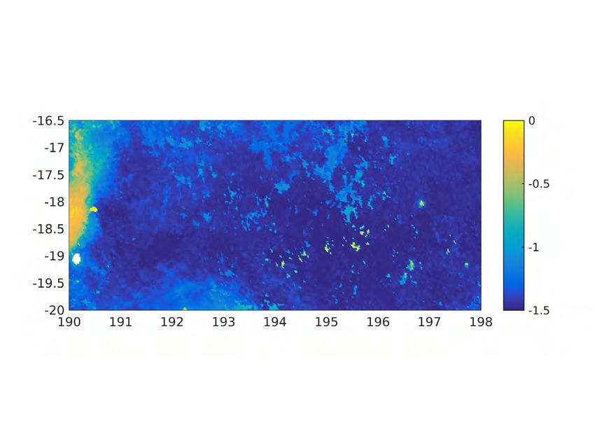
2130                                                                                          A. de Verneil et al.: LD OUTPACE

chosen because post-processed CTD casts did not always in-             The statistical baseline was defined as a functional fit be-
clude the surface.                                                  tween σθ and spice measurements at the beginning of each
   The SedTrap Drifter had six SBE 37 Microcat CTDs on              LD station in the upper 200 m of the water column spanning
board. Their depths, as determined by mean in situ pressure,        the euphotic zone. The period of time used for defining the
were ∼ 14, 55, 88, 105, 137, and 197 m. These instruments           baseline was chosen to be the local inertial period, so that
yielded data every 5 min during their deployments. As men-          internal wave effects would be minimized. For each station,
tioned in the previous paragraph, during LDA the SedTrap            this meant that the first 13, 15, and 15 casts were used for
Drifter tangled with the production line and so the data pre-       LDA, LDB, and LDC, respectively. A regular grid of den-
sented here from LDA came from its redeployment until the           sity values was created, with one fourth of the number of
end of LDA. No gap in the data occurred for LDB or LDC.             values as the total number of observations. The fit of base-
                                                                    line spice, or Sbase (ρ), was calculated inside a moving win-
                                                                    dow of ±0.1 kg m−3 along with the standard error in spice,
2.4.2   Tracer analysis and baseline definition
                                                                    SErrbase (ρ). Only values corresponding to windows with at
                                                                    least 50 observations were kept.
The need for a baseline within the OUTPACE dataset can                 Comparisons between the baseline and new σθ -spice mea-
be shown by comparison of the CTD data with climatolo-              surements were made using a Z-Score, following the general
gies such as the World Ocean Atlas (Fig. S1 in the Sup-             formula as follows:
plement; Boyer et al., 2013). While OUTPACE observations
                                                                                 Sobs − Sbase
were consistent with these previous observations, when met-         Z(ρobs ) =                ,                                  (1)
rics of variability were available they produced envelopes of                     SErrbase
max/min T -S values large enough to preclude distinguish-           where, for a density observation ρobs , Sobs is the observed
ing between different stations. Since no other sufficiently fine    spice with Sbase and SErrbase being the linearly interpolated
data were available to compare T -S measurements, data from         functional baseline spice value and standard error. The as-
within each station were used to create a reference baseline        sumption applied in this analysis is that while a continuous
of T -S variability. Given the lack of fine variability data and    curve in T -S, or σθ − S, is to be expected and can be fit to
the need to work within the dataset of a single cruise, an-         a function, the isopycnal layers were independent of each
other approach was needed to condense T -S variability so           other, and represented different physical sub-populations.
that physical environments can be distinguished.                    Keeping track of variability through Z-score tied to a func-
   Generally, over the upper 200 m of the water column, the         tional σθ −S relationship produced a flexible metric. For sen-
depth range of most of our CTD casts, a given profile of T -        sors fixed at a certain depth, such as for the SedTrap drifter, a
S values will vary along a curve (Stommel, 1962). This re-          Z-score could be computed irrespective of whether internal
flects how each profile is made up of increasingly denser lay-      waves were shoaling or deepening isopycnals.
ers over depth, each with distinct histories. In some sense,
these layers could be considered their own physical micro-          2.5   Spatial scale determination and baseline context
environment, and their ensemble constitutes the physical en-
vironment. Assuming that the density layers were not subject        The Z-scores derived from the CTD and SedTrap time se-
to strong forcing, such as diapycnal mixing events or atmo-         ries provided a first-order evaluation of physical variability
spheric effects, their values should have remained constant         in the immediate surroundings of the SedTrap drifter as it
until isopycnal exchange or diffusion could occur over longer       moved through time. If large variability (|Z| > 2, in the tra-
timescales. Treating these density layers as separate entities,     ditional α = 0.05) was observed, then the physical environ-
variations of T -S along isopycnal surfaces can provide an          ment likely had changed. However, if |Z| < 2 this was not
approach to distinguish physical environments, which is the         a guarantee that the physical environment had not changed.
goal of our analysis.                                               Since the functional fit of σθ and spice was based only upon
   Using density as one variable, another is needed to fully        the data from OUTPACE, Z-score is a relative measure of
describe a water parcel’s characteristics, ideally one which        variability. In order to test whether the σθ -spice relationship
is independent of density. Spice, a variable constructed from       was robust, it was necessary to extend the Z-score analysis
T -S, is well suited for this purpose. Spice is defined such that   farther in space to include complementary density and spice
hot and salty water is “spicy”, a convention dating to Munk         measurements. If Z-scores remained low for large distances,
(1981). In the formulation proposed by Flament (2002), its          then the SErrbase was too large. By compiling independent
isopleths are perpendicular to isopycnals everywhere, and it        Z-scores over larger distances, we can test whether there is a
effectively both encapsulates and accentuates T -S variability      relationship between Z-score and distance.
at a given density into a single value. Therefore, in our anal-        During OUTPACE, complementary σθ -spice observations
ysis, spice variability in a given density layer was used to de-    stemmed from neighboring stations, the SD stations (Fig. 1).
fine the statistical baseline and determine whether a physical      Additionally, surface measurements for the entire cruise were
environment changed during OUTPACE.                                 provided from a Seabird SBE 21 SeaCAT thermosalinograph

Biogeosciences, 15, 2125–2147, 2018                                                       www.biogeosciences.net/15/2125/2018/
A. de Verneil et al.: LD OUTPACE 2131
(TSG), with SBE 38 thermometer using the ship’s continuous Trap Drifter. The post-processed AQUADOPP time series
surface water intake. Subsequent to post-cruise processing of provided observations every 5 min.
TSG data as detailed in Alory et al. (2015), the time series Velocities were integrated using a first-order Euler method
was available in 2 min intervals. to calculate the theoretical trajectories of water subsequent to
The relationship between Z-score vs. distance was used the beginning of each LD station. Since the object of these
to evaluate the baseline. Distances were calculated from the calculations was to see whether water could have traveled a
ship position of observation and the initial CTD cast posi- critical spatial scale, for each dataset the maximal amount of
tion for the LD station. For the SD stations, the Z-scores time was given for the time integration. SADCP time series
found by the functional fit of spice for each cast were binned spanned between the first and last CTD of the LD station, us-
by density, in a regular grid with bins of 0.25 kg m−3 width. ing the ship position as the initial position. The AQUADOPP
TSG data from during the LD stations were excluded and integrations spanned the entirety of valid data and used the
Z-scores were binned by distance from the station, in 10 km corresponding SedTrap Drifter satellite fix for an initial po-
increments for the first 100 km, and then 20 km afterwards sition.
until 500 km. The spatial scale RZ was determined where To compare the integrated velocity positions with the real-
Z ≥ 2 and used to evaluate the ability of the statistical base- ized positions of the SedTrap drifter and SVP drifters, GPS
line to discern gradients in physical properties. A natural spa- positioning was achieved by use of Iridium telemetry. Posi-
tial scale to serve as a useful reference to the empirical dis- tions were successfully found for LDA before and after the
tance is the first Rossby radius of deformation, approximated SedTrap Drifter’s redeployment, along with all of LDB. Dur-
via Wentzel–Kramers–Brillouin (WKB) method by Chelton ing LDC, the battery of the positioning antenna ran out and so
et al. (1998) as follows: the time series for LDC positions of the SedTrap Drifter was
shortened. Since only the initial position is needed for the
1 0
Z
RD = N (z)dz, (2) velocity integration, the AQUADOPP integration was contin-
πf −H ued beyond this positioning failure until the SedTrap Drifter
where f is the local coriolis parameter and N (z) is the depth- was recovered. Positions of the SVP drifters deployed at each
dependent Brunt–Väisälä frequency. RD was calculated for station were successfully retrieved for all three LD stations.
each LD station using the deepest cast available: 2000 m Satellite fixes were available spaced about 1 h apart for both
casts for LDA and B, and a deep 5000 m cast for LDC. N datasets. Both SedTrap Drifter and SVP positions were in-
was calculated with centered differences of the 1 m binned terpolated to hourly time series. SVP positions were used to
density profiles. compute relative dispersion (Fig. S2 in the Supplement), us-
ing the definition for N particles as follows (LaCasce, 2008):
2.6 Currents analysis and Lagrangian risk
1 XN
D(t) = [x (t) − xj (t)]2 ,
i6=j i
(3)
The previous step analyzed the relationship between Z-score 2N (N − 1)
and distance, providing an estimated distance over which the
where N here is the total number of SVP drifters and x the
physical environment changed. In order to evaluate the risk
time series of the drifter i’s x, y position.
that the SedTrap drifter encountered different water masses,
an analysis of the local currents was needed. Since it is clear
that the SedTrap drifter was not perfectly Lagrangian and that 3 Results
vertical shear could transport layers at different rates, it was
necessary to see if water at specific depths could have ad- 3.1 Satellite data, temporal context, and method
vected the distance over which different water masses appear. applicability
The in situ velocities for each LD station were de-
rived from the shipboard acoustic Doppler current profilers The regional distributions of SST and surface chl a as seen
(SADCP), two ocean surveyors at 150 and 38 kHz. Time during the OUTPACE cruise are shown in Fig. 1. The data in
series data for the SADCPs were post-processed using the Fig. 1 are weighted means, with the weight being the inverse
CASCADE software package (Le Bot et al., 2011; Lher- square of the ship’s daily distance to each pixel. A north–
minier et al., 2007) and binned into 2 min intervals. The south meridional gradient was found in SST, with warmer
150 kHz SADCP provided a depth resolution of 8 m, with water near the equator (∼ 30 ◦ C) and cooler water poleward
bins starting from 20 m, and reliable data coverage down to (∼ 25 ◦ C). This gradient was uninterrupted for the duration
200 m depth. Since the SedTrap Drifter had sediment traps of the OUTPACE cruise. Due to the zonal ship track the sur-
extending down to 500 m depth, the 38 kHz data was also face thermal conditions observed by the ship during OUT-
used, albeit with reduced depth resolution of 24 m bins, ex- PACE were relatively homogeneous. Furthermore, no strong
tending from 52 m down to 1000 m. Additional in situ ve- temperature gradients, indicative of frontal or eddy struc-
locities came from six Nortek AQUADOPP current meters, tures, were visible in the vicinity of the stations. While a
positioned at 11, 55, 88, 105, 135, and 198 m on the Sed- north–south regional gradient was found in SST, the opposite
www.biogeosciences.net/15/2125/2018/ Biogeosciences, 15, 2125–2147, 20182132 A. de Verneil et al.: LD OUTPACE
size of the bloom was large enough to cover most of the
(a)-17.5 1
120 km×120 km region shown in Fig. 2b, so the bloom edges
-18 were far away from station LDB’s initial position. By con-
Chl a (mg m-3)
SD2
Latitude (° N)
-18.5 trast, waters outside the bloom had chl a values lower than
0.32
-19 SD3 in Fig. 2a. The low chl a values near LDC in Fig. 2c were
-19.5
SD4 typical of the SPG, and no visible patches of chl a indicated
0.1
-20 sharp gradients.
-20.5 The time series of chl a and SST for the three stations
-21 0.03 are shown in Fig. 3. Comparing the three LD stations, a few
(b) -17 162 163 164 165 166 167 168
1 patterns emerge. SST showed similar trends across the three
-17.5
LD stations. All stations experienced warming trends from
December 2014 to mid-March 2015, consistent with sum-
Chl a (mg m-3)
Latitude (° N)
-18
0.32 mer heating. The lack of data from cloud cover sometimes
-18.5 SD13 led to abrupt drops in the distribution of daily SST shown.
-19 SD12 However, the timing of maximum temperature and the mag-
0.1
-19.5 nitude of that warming did differ between LD stations. A
-20 rapid heating in December 2014 occurred around LDA’s po-
-20.5 0.03
sition, which then slowly continued until early March 2015,
186 187 188 189 190 191 192 at which point temperatures began to drop. Towards the
(c)-16.5 1 end of sampling at station LDA the SST rises, possibly in-
Chl a (mg m-3)
-17 dicating another warming event occurred or the arrival of
Latitude (° N)
-17.5
SD13 0.32 a warm patch of water. Depth-resolved application of our
-18 SD14
method in the later sections will evaluate this possibility.
-18.5
-19
0.1 The overall evolution in LDA’s temperature during the period
-19.5 shown, from ∼ 26 to 30 ◦ C, represented a 4 ◦ C change. LDB
-20 0.03 showed a slight cooling in December 2014, but this may have
190 191 192 193 194 195 196 197 198
been an artifact of cloud cover. Station sampling for LDB
Longitude (°E) occurred immediately after the maximum heating, though
the values seen at LDB were relatively stable and slightly
Figure 2. Satellite chl a around (a) LDA, (b) LDB, and (c) LDC. SD warmer than at LDA. The maxima in temperature for LDA
stations shown by black crosses, land is shaded gray, and coastlines and LDB seemed to overlap in time in early March 2015.
and reefs are plotted in black. LD stations shown by plus symbols LDB’s change in temperature, from ∼ 27 to 30 ◦ C, was a
following the color code from Fig. 1. Squares with 120 km to a side
3 ◦ C change. LDC had the smallest change in temperature,
plotted around each LD station to represent approximate Rossby
from ∼ 27 to 29 ◦ C for a 2 ◦ C change. Sampling for LDC
radius RD .
coincided with the warmest period observed in the satellite
data, in late March 2015, and was stable for the LD sampling
period.
was found in chl a. Chl a values were around 0.3 mg m−3 in The timing of temperature maxima is important to note
the western portion of the domain, west of 190◦ E. Stations for biological reasons, since N2 fixation by Trichodesmium
LDA and LDB were in this region, with LDB positioned in- spp. is known to occur in warm, stratified waters (specifically,
side a bloom with values near 1 mg m−3 . More details con- a ∼ 25 ◦ C threshold, White et al., 2007) and one of the goals
cerning the LDB bloom can be found in de Verneil et al. of OUTPACE was to observe this biogeochemical process.
(2017). Chl a values dropped precipitously, over an order of Since SST was above 25 ◦ C for all stations throughout this
magnitude to 0.03 mg m−3 , just east of LDB near LDC. The period, the thermal conditions during OUTPACE would not
low value of chl a was indicative of the South Pacific Gyre have limited N2 fixation.
(SPG; Claustre et al., 2008). In between December 2014 and January 2015, the region
Since SST was relatively unchanging during OUTPACE, around LDA had higher chl a concentrations than LDB. The
Fig. 2 provides zoomed-in views of the chl a data for the period between February and May 2015 showed a remark-
three LD stations, with domains chosen to include the near- able increase in chl a near the LDB site. This was due to ad-
est SD stations. The spacing of the SD stations was relatively vection of the surface bloom, which subsequently collapsed
regular along the OUTPACE transect (Fig. 1b). In Fig. 2a and advected away, as documented in another study in this
the enhanced chl a was distributed evenly inside the do- special issue (de Verneil et al., 2017). The downward trend
main, so no clear surface gradients are present. In Fig. 2b, of chl a during this period is more indicative of in situ evo-
the chl a was concentrated in the aforementioned bloom, lution, rather than advection of the bloom’s boundaries, and
with values higher than those seen in Fig. 2a near LDA. The does not invalidate subsequent use of our method. Near LDC,
Biogeosciences, 15, 2125–2147, 2018 www.biogeosciences.net/15/2125/2018/A. de Verneil et al.: LD OUTPACE 2133
(a) Surface Chl D (b) SST
% pixels
Chl D (mg m-3 ) % pixels
100 100
50 50
0 0
1 31
LDA
0.8
SST (°C)
29
0.6
0.4
27
0.2
0 25
(c) (d)
12/1/14 1/1/15 2/1/15 3/1/15 4/1/15 5/1/15 12/1/14 1/1/15 2/1/15 3/1/15 4/1/15 5/1/15
% pixels
Chl D (mg m-3 ) % pixels
100 100
50 50
0 0
1 31
LDB
0.8
SST (°C)
29
0.6
0.4
27
0.2
0 25
(e) 12/1/14 1/1/15 2/1/15 3/1/15 4/1/15 5/1/15
(f)
12/1/14 1/1/15 2/1/15 3/1/15 4/1/15 5/1/15
% pixels
Chl D (mg m-3 ) % pixels
100 100
50 50
0 0
1 31
LDC
0.8
SST (°C)
29
0.6
0.4
27
0.2
0 25
12/1/14 1/1/15 2/1/15 3/1/15 4/1/15 5/1/15 12/1/14 1/1/15 2/1/15 3/1/15 4/1/15 5/1/15
Date Date
Figure 3. Time series of surface chl a and SST, respectively, for (a, b) LDA, (c, d) LDB, and (e, f) LDC. Intervals of LD sampling shown
with gray dashed lines. Mean values are plotted in black, with darker shades representing the 25–75 % interval and lighter shades for 1–99 %.
Subpanels above each time series depict the % of pixels with data. All data come from within the 120 km × 120 km squares shown in Fig. 2.
chl a was systematically low, a reflection of the goals of also determine whether the surface increase in SST during
OUTPACE to sample in the SPG. LDA was reflective of changes at depth. As a final note,
Besides the increase in SST at the end of LDA and the Rousselet et al. (2018) found with satellite-derived surface
decrease in chl a during LDB, both SST and chl a for the velocities that during LDC a coherent structure was present,
LD stations were stable, providing evidence that no surface despite the lack of surface SST and chl a gradients. Since
gradients, physical or biological, immediately invalidate the tracer gradients are non-existent at the surface, we find that
application of our strategy. Though the change in chl a at this is not a strong structure, and does not invalidate the ap-
LDB has been argued to be due to endogenous dynamics in plicability of our approach. Rather, the application of depth-
the aforementioned study, application of our post-validation resolved in situ measurements of tracers and velocities will
method provides an independent test of whether advection serve as an independent evaluation of this finding.
of gradients could be responsible. Likewise, the method will
www.biogeosciences.net/15/2125/2018/ Biogeosciences, 15, 2125–2147, 20182134 A. de Verneil et al.: LD OUTPACE
(a) (b) (c)
Pref = 0 dBar Pref = 0 dBar Pref = 0 dBar
30 22 30 22 30 22
Conservative temperature Θs (°C)
28 28 28
6 6 6
26 23 26 23 26 23
5 5 5
24 24 24
24 24 24
22 4 22 4 22 4
20 20 20
25 25 25
3 3 3
18 18 18
16 16 16
Legend Legend Legend
26 LDA SD2 26 LDB SD12 26 LDC SD13
14 SD3 SD4 14 SD13 14 SD14
35 35.4 35.8 36.2 35 35.4 35.8 36.2 35 35.4 35.8 36.2
Absolute salinity Sₐ (g kg -1) Absolute salinity Sₐ (g kg -1) Absolute salinity Sₐ (g kg -1)
Figure 4. T -S diagrams of (a) LDA, (b) LDB, and (c) LDC and surrounding stations. LD stations are color coded, and SD stations different
shades of gray. Isopycnals are displayed in black, with isopleths of spice shown in red.
3.2 In situ properties, statistical baseline, and time 7
series analysis
6
The hydrographic variability during the three LD stations and
surrounding SD stations are shown in the T -S diagrams of
Spice
Fig. 4. All three stations followed a general pattern, where
surface water near the 1022 kg m−3 isopycnal and 29 ◦ C tem- 5
perature (though LDB had warmer surface water, Fig. 4b)
dropped in temperature and increased in salinity until a sub- Legend
surface salinity maximum near the 1025 kg m−3 isopycnal. 4
LDA
The increase in salinity maximum from LDA to LDC reflects LDB
the high salinity tongue of the South Pacific (Kessler, 1999). LDC
The surface water in LDA (Fig. 4a) showed a bifurcation.
3
This change was manifest in the satellite data time series, as 1022 1023 1024 1025
-3
well. Whether this is due to a heating event or the arrival of Density (kg m )
new water at the end of LDA will be addressed in the time
series analysis below. For LDA, neighboring stations SD2, Figure 5. Statistical LD baseline of spice versus potential density
3, and 4 largely overlapped with the LDA profile. SD3, the for (a) LDA, (b) LDC, and (c) LDC. Mean values plotted in between
station closest to LDA, almost entirely overlapped the LD envelope of ±2 SErrobs .
profile, except for a subsurface salinity deviation below the
1024.5 kg m−3 isopycnal. SD2 and SD4 showed greater de-
viations, with SD4 being saltier than LDA for almost the en- Additionally, the saltier nature of LDC relative to LDA and
tire profile. Similar overlaps occurred with LDB and its sur- LDB, especially between 1024 and 1025 kg m−3 , was visible.
rounding stations, SD12 and SD13 (Fig. 4b). SD12 showed The variability in T -S values between stations was within the
lower salinity near the surface, with a kink in salinity at the range seen in the climatology of the region (Figs. S1 and S2).
1025 kg m−3 isopycnal. The salinity offsets of SD4 and SD12 The LD statistical baselines of spice in density space, with
at depth are within climatological variability (Figs. S1 and means and intervals of two standard errors, are shown in
S2). SD13 had similar surface structure to LDB, but higher Fig. 5. These standard error intervals, representing the in-
salinities from the 1023.5 to 1025 kg m−3 isopycnal. The herent variability in the baseline, show the values wherein
LDC, SD13, and SD14 (Fig. 4c) profiles nearly entirely over- a Z-score of ≤ 2 was achieved. LDB and LDC overlapped
lapped except near the surface when the SD stations were for essentially their entire profiles. All stations are missing
at first less salty at the surface and then became more salty. observations near the surface and mixed layer due to the in-
Biogeosciences, 15, 2125–2147, 2018 www.biogeosciences.net/15/2125/2018/A. de Verneil et al.: LD OUTPACE 2135
(a) (b)
4
2
Z-score
0
-2
-4
(c) (d)
4
2
Z-score
0
-2
-4
(e) (f)
4
2
Z-score
0
-2
-4
F-26 F-27 F-28 M-01 M-02 F-26 F-27 F-28 M-01 M-02
Time Time
Figure 6. SedTrap drifter Z-score time series for (a) 14, (b) 55, (c) 88, (d) 105, (e) 137, and (f) 197 m depth. End of inertial period timeframe
for baseline definition plotted in magenta. Z = −2 and 2 plotted in black.
tense stratification which left several density bins with less in LDC shows similar widening as in LDB, with a noticeable
than 50 observations, the threshold used in the spice analysis. pinch in the envelope near 1024.5 kg m−3 .
LDA was noticeably less spicy than the other two LD stations The Z-score time series for the SedTrap Drifter sensors are
for density less than 1024 kg m−3 . At the highest densities, shown in Figs. 6–8. During LDA, at 14 m depth (Fig. 6a), af-
all three LD stations overlapped. The envelope of two stan- ter the inertial period baseline determination the Z-score first
dard errors, or Z-score ≥ 2, show that variability has some descended, increased, and then leveled off after the first two
dependence on depth. The LDA baseline shows high vari- and a half days. Afterwards, the Z-score increased, reach-
ability near the surface, with a thin envelope below down to ing 2, decreased, and surpassed Z = 2 before falling again.
1024 kg m−3 , and widening at depth down to 1025 kg m−3 The SedTrap drifter at 55 m showed no trend (Fig. 6b), and
and beyond. LDB did not have high surface variability, but a single Z-score was seen below −2. Z-scores for 105, 137,
the envelope widens shortly below 1023 kg m−3 . Variability and 197 m (Fig. 6d–f) showed no temporal trends and were
always less than 2 in magnitude. The time series at 88 m
www.biogeosciences.net/15/2125/2018/ Biogeosciences, 15, 2125–2147, 20182136 A. de Verneil et al.: LD OUTPACE
(a) (b)
2
Z-score
0
-2
(c) (d)
2
Z-score
0
-2
(e) (f)
2
Z-score
0
-2
M-16 M-17 M-18 M-19 M-20 M-16 M-17 M-18 M-19 M-20
Time Time
Figure 7. Same as Fig. 6 but for LDB.
showed no trend but the variability in Z-score increased over LDC. Z-scores at 55, 137, and 197 m showed no trends in Z-
time, with some observations surpassing |Z| = 2. score, and had limited observations with |Z| > 2. At 88 m, no
LDB SedTrap drifter Z-scores (Fig. 7) showed similar pat- trend was seen, and for the first two days there were few ob-
terns to LDA. The surface sensor (Fig. 7a) decreased and in- servations with Z < −2. Toward the end of LDC, two spikes
creased over the first two days, then leveled with temporary with Z > 2, with Z ∼ 4–5, occurred with returns back to
departures below −2. The sensors at 55, 105, 137, and 197 m |Z| < 2. The Z-scores at this depth ended near Z = 2. Ob-
(Fig. 7b, d–f), similar to LDA showed no trends and low vari- servations at 105 m started around −2 < Z < 0, but spikes
ability. A few observations below −2 occurred at 55 m. The with Z ∼ 2 occurred. Over time, Z-scores trended upward
Z-scores at 88 m showed no trend, similar to LDA with en- with more oscillations, with a shift to Z > 2 becoming dom-
hanced variability and some |Z| > 2 but no time-dependence. inant during and following 27 March 2015.
The LDC Z-scores were large at more depths than the CTD Z-score time series are shown for LDA, LDB, and
other LD stations (Fig. 8). Values at 14 m started with Z > 2, LDC in Figs. 9, 10, and 11, respectively. LDA Z-scores
but that dropped before rising again after a day, before slowly were generally |Z| < 2, but Z-scores for densities σθ <
dropping and eventually decreasing to ∼ −2 at the end of 1022 kg m−3 were greater than 2 starting 1 March, and con-
Biogeosciences, 15, 2125–2147, 2018 www.biogeosciences.net/15/2125/2018/A. de Verneil et al.: LD OUTPACE 2137
(a) (b)
6
4
2
Z-score
0
-2
-4
-6
(c) (d)
6
4
2
Z-score
0
-2
-4
-6
(e) (f)
6
4
2
Z-score
0
-2
-4
-6
M-24 M-25 M-26 M-27 M-28 M-24 M-25 M-26 M-27 M-28
Time Time
Figure 8. Same as Fig. 6 but for LDC.
tinued for the rest of the station. The increasing trend in during 26 March, but as time went on a larger swath of den-
Z-score near the surface was also reflected in the SedTrap sity had |Z| > 2 and this change was largely permanent. Near
drifter. LDB CTD Z-scores showed almost no observations 1025 kg m−3 , a separate series of large Z-scores appeared on
with |Z| > 2. These occurred at the surface with low densi- 27 March and lasted for most of the rest of LDC.
ties and a few near σθ ∼ 1023.25 kg m−3 . All these observa-
tions occurred before or around 19 March and no temporal 3.3 Spatial scale and baseline context
trend in |Z| > 2 was seen. The Z-scores for LDC showed
similar trends to the SedTrap drifter. Near the surface close The TSG Z-scores for the three LD stations are shown in
to σθ ∼ 1022 kg m−3 , |Z| > 2 was seen early in the time Fig. 12. For LDA, Z > 2 occurred at 150 km. Z-scores were
series, but then dropped to |Z| < 2 until another increase consistently large farther away from this point. The LDB
around 27 March. This pattern was similar to the SedTrap TSG surpassed Z = 2 at 55 km, though Z-score diminished
drifter’s observations at 14 m. Regions of |Z| > 2 appeared again 300 km away. For LDC, TSG Z-score reached 2 at
in the 1024–1025 kg m−3 range, primarily during 27 March. 35 km distance, and |Z| oscillated between larger and less
A small density range near 1024.5 kg m−3 showed |Z| > 2 than 2 farther away. Therefore, at the surface layer, 150, 55,
www.biogeosciences.net/15/2125/2018/ Biogeosciences, 15, 2125–2147, 20182138 A. de Verneil et al.: LD OUTPACE
M-02 M-28
Time (Mo-day)
Time (Mo-day)
M-01 M-27
M-26
F-28
M-25
F-27 Legend
Legend
Inertial period Inertial period
Observation Observation
M-24
F-26 |Z| > 2 |Z|>2
1022 1023 1024 1025 1026
1022 1023 1024 1025 -3
Density (kg m )
Density (kg m-3)
Figure 11. Same as Fig. 9 for LDC, with |Z| < 2 observations plot-
Figure 9. Time series of CTD observations for LDA. Observations ted in blue.
with |Z| < 2 plotted in green, |Z| > 2 in black. End of statistical
baseline definition period shown in magenta.
500
450
400
Distance (km)
M-20 350
300
Time (Mo-day)
250
M-19 200
150
M-18 100
50
0
M-17
LDB
LDC
LDA
Legend
Inertial period
Observation
M-16 |Z|>2
Figure 12. TSG Z-score over distance for LDA (left, green), LDB
(center, red), and LDC (right, blue). |Z| > 2 is shaded black. Rossby
radii RD distance plotted in horizontal dashed lines, color coded to
1022 1023 1024 1025 the LD stations.
-3
Density (kg m )
Figure 10. Same as Fig. 9 for LDB, with |Z| < 2 observations plot- Z-scores from the SD stations are presented in Fig. 13.
ted in red. For LDA, the |Z| > 2 distances demonstrated density depen-
dence. Near 1022 kg m−3 , |Z| > 2 immediately, at ∼ 45 km,
though this did not occur at the surface. Approaching
and 35 km were the spatial scales. Since at least some Z- 1000 km distance, |Z| > 2 occurred from the surface to
scores were found to be greater than 2, the baseline was sen- 1024 kg m−3 . By 3500 km, all density layers show |Z| > 2.
sitive enough to determine gradients over a 500 km scale. LDB showed large Z-scores in some density layers at the
Since Z-scores for LDB and LDC were not consistently closest SD station located 189 km away. Past 750 km, Z
|Z| > 2, then the baseline’s sensitivity was perhaps not as from 1022–1024 kg m−3 was consistently high. For densities
great as LDA. The Rossby radii for the three stations were greater than 1024 kg m−3 , Z-scores were enhanced between
46.5, 48.8, and 60 km. The spatial scales for the TSG data 1000 and 1500 km, but then decreased farther away. LDC’s
at LDB and LDC matched up to the Rossby radii, whereas Z-scores show that |Z| was greater than 2 from the first ob-
LDA’s TSG data indicated a larger scale. servations at 310 km. All density layers showed enhanced
Biogeosciences, 15, 2125–2147, 2018 www.biogeosciences.net/15/2125/2018/A. de Verneil et al.: LD OUTPACE 2139
(a) (b) (c)
4000
3000
Distance (km)
2000
1000
0
1022 1023 1024 1025 1022 1023 1024 1025 1022 1023 1024 1025
Densit y (kg m-3) Densit y (kg m-3) Densit y (kg m-3)
Figure 13. SD station Z-score over distance for (a) LDA, (b) LDB, and (c) LDC. |Z| > 2 shaded black. Rossby radii RD distance plotted in
horizontal lines, color coded to the LD stations.
Z values, with the majority of all observations being larger son, the 150 kHz 52 m time series produced u, v correla-
than 2. Similar to the TSG data, the SD stations showed that tions with the AQUADOPP of 0.83 and 0.80 (LDA); 0.00
the baselines were sufficiently sensitive to detect physical and 0.02 (LDB); and 0.68 and 0.68 (LDC). Vector correla-
gradients on large scales, with some detecting changes im- tions using the method of Crosby et al. (1993) for the three
mediately. Putting together the near-surface TSG data and time series (not reported) similarly showed a maximum for
CTD data from the SD stations, LDA showed smaller |Z| = 2 LDA, minimum near-zero for LDB, and low values for LDC.
scales at depth, whereas LDB and LDC both showed variabil- These differences likely result from higher frequency fluctua-
ity both near the surface and at depth at smaller scales. In or- tions of the currents, at the inertial and tidal frequencies. The
der to be the most conservative in our velocity and trajectory fact that a higher correlation is obtained at LDA is probably
estimates, we will use the smallest spatial scale of |Z| = 2 to partly the consequence of the larger horizontal scales of the
determine the spatial scale RZ and evaluate Lagrangian risk, near-inertial signal dominant at LDA compared to the baro-
namely 45 km for LDA, 55 km for LDB, and 35 km for LDC. clinic tidal signal, e.g., resulting from the dispersion relation
Having evaluated the ability of the statistical baselines to (Alford et al., 2016). These oscillations, and their implica-
sense physical gradients over large scales, we are now ready tions for turbulent mixing, are analyzed in greater detail in
to analyze the currents and trajectories. Bouruet-Aubertot et al. (2018).
The disagreement between the two velocity data sources
3.4 Velocities and Lagrangian trajectories had an impact on the integrated trajectories. Take, for ex-
ample, a closer inspection of the SADCP and AQUADOPP
Time series of the 38 kHz SADCP and AQUADOPP data are during LDA, which had the strongest currents. The initial
presented in Fig. 14. The LDA time series of SADCP u and v positions of the ship and the SedTrap Drifter were 1.46 km
components (Fig. 14a, d) showed strong near-inertial oscilla- apart. After 3 days and 2 h, the AQUADOPP integration
tions in the upper 200 m, with velocities reaching magnitudes had traveled 67.75 km, the SADCP 60.71 km with a final
of 0.6 m s−1 . A weaker tidal component was also present in separation of 10.89 km. The result was a positional drift of
this layer: below 200 m, vertical columns of alternating ve- ∼ 3 km day−1 , or an average increase in position difference
locity sign indicated the semi-diurnal tide. These tidal sig- of 147 m for each km traveled. A similar analysis for the
natures were also the dominant signal in the LDB and LDC LDB time series, with weaker currents but essentially no cor-
time series (Fig. 14b–c, e–f). The mixed layer, which, for relations over 4 days and 15 h, resulted in a positional drift
most of the cruise, was ≤ 20 m, was not resolved by either of 3.19 km day−1 , with an increased position difference of
SADCP. So, the near-surface velocities were only captured 318 m for each km traveled. Thus, a lower correlation time
by the 11 m AQUADOPP and the SVP drifters drogued at series, but with lower magnitudes, resulted in similar misfit
15 m. Comparing the 55 m AQUADOPP time series with the in the integrated trajectory.
52 m SADCP, the two data sources displayed similar trends The trajectories of the integrated velocities, as well as ob-
for LDA. The strong near-inertial oscillations led to corre- servations of SedTrap Drifter and SVP positions, are pre-
lations between the AQUADOPP and 38 kHz time series of sented in Fig. 15. The average altimetry-derived currents sug-
0.75 and 0.76 for the u and v components, respectively. Dur- gested there should be recirculation around the positions of
ing LDB and LDC, the weaker currents did not correlate LDA and LDC, whereas LDB had a mean northward flow
as well, leading to u, v correlations of −0.0137, −0.0554 (Fig. 15a–c). The SedTrap Drifter trajectory for LDA did not
(LDB), and 0.30, 0.37 (LDC), respectively. For compari-
www.biogeosciences.net/15/2125/2018/ Biogeosciences, 15, 2125–2147, 2018You can also read