Paleozoic-Mesozoic Eustatic Changes and Mass Extinctions: New Insights from Event Interpretation - MDPI
←
→
Page content transcription
If your browser does not render page correctly, please read the page content below
life

Article
Paleozoic–Mesozoic Eustatic Changes and Mass
Extinctions: New Insights from Event Interpretation
Dmitry A. Ruban
 K.G. Razumovsky Moscow State University of Technologies and Management (the First Cossack University),
 Zemlyanoy Val Street 73, 109004 Moscow, Russia; ruban-d@mail.ru

 Received: 2 November 2020; Accepted: 13 November 2020; Published: 14 November 2020

 Abstract: Recent eustatic reconstructions allow for reconsidering the relationships between the
 fifteen Paleozoic–Mesozoic mass extinctions (mid-Cambrian, end-Ordovician, Llandovery/Wenlock,
 Late Devonian, Devonian/Carboniferous, mid-Carboniferous, end-Guadalupian, end-Permian, two
 mid-Triassic, end-Triassic, Early Jurassic, Jurassic/Cretaceous, Late Cretaceous, and end-Cretaceous
 extinctions) and global sea-level changes. The relationships between eustatic rises/falls and period-long
 eustatic trends are examined. Many eustatic events at the mass extinction intervals were not anomalous.
 Nonetheless, the majority of the considered mass extinctions coincided with either interruptions or
 changes in the ongoing eustatic trends. It cannot be excluded that such interruptions and changes
 could have facilitated or even triggered biodiversity losses in the marine realm.

 Keywords: biotic crisis; global sea level; life evolution

1. Introduction
      During the whole Phanerozoic, mass extinctions stressed the marine biota many times. They triggered
disappearances of numerous species, genera, families, and even high-order groups of marine organisms,
and they were often associated with outstanding environmental catastrophes such as global events
of anoxia and euxinia, unusual warming and planetary-scale glaciations, massive volcanism, and
extraterrestrial impacts. Mass extinctions were highly complex events, with the intensity amplified by
the interplay among atmosphere, oceans, geologic activity, and extraterrestrial influences. The relevant
knowledge is huge, and it continues to grow. Importantly, this knowledge growth is indivisible from
the progress in the understanding of marine (paleo)ecosystems and (paleo)environments, both at
the global and local scales. The most important contributions that formed the very fundamentals
of what can be called “mass extinction science” were made by Bambach [1], Benton [2,3], Clapham
and Renne [4], Elewa and Abdelhady [5], Erwin [6], Hallam [7], Jablonski [8], Holland [9], Melott
and Bambach [10], Racki [11], Rampino and Caldeira [12], Raup and Sepkoski [13], Thomas [14],
Twitchett [15], and Wignall [16]. Hundreds of other researchers have also contributed substantially
and focused on particular catastrophic events, fossil groups, or extinction factors.
      Eustatic (global sea-level) changes have been regarded as a debatable cause of mass extinctions for
decades [17–21]. However, currently, there is not consensus about the relevance of this cause. This is due
to stratigraphical record biases, the complexity of mechanisms linking eustasy and marine biodiversity
changes, and “chaos” in global sea-level interpretations [22]. Often, restriction of the analyses to only
regional or even local records and confusion between transgressions–regressions (“horizontal” changes)
and sea-level rises–falls (“vertical” changes) also matter. Moreover, substantial improvements in the
geologic time scale and eustatic reconstructions require permanent re-consideration of earlier research,
which is undermined by the unpopularity of theorizing in modern geology [23]. One may even
question the very sensibility of special studies of the eustatic factor of mass extinction. Nonetheless,
this factor cannot be ignored. Whether global sea-level changes were able to trigger mass extinctions,

Life 2020, 10, 281; doi:10.3390/life10110281                                      www.mdpi.com/journal/life
Life 2020, 10, 281 2 of 14
it appears undisputable that the position and tendencies of the global sea level was one of the
environmental conditions that could either reduce or facilitate the biodiversity loss during mass
extinction events. In other words, the eustatic setting of mass extinctions requires proper examination.
A significant question is whether this research direction should shift from qualitative interpretations
(visual interpretations of curves depicting changes of biodiversity and sea level) to more quantitative
(statistical) analyses. Although the latter seem to be more advanced than the former, three reasons
should be taken into consideration. First, statistical analyses need conceptual frameworks. Second,
the selection of biotic crises for analysis is a subjective procedure due to various biases in the available
knowledge. Third, qualitative analyses of the mass extinction causes persist in current geoscience
research, whereas quantitative analyses are essentially not so new [24,25]. The importance of the
periodicity/cyclicity studies by Melott and Bambach [10], Rampino and Caldeira [12], Roberts and
Mannion [20], Boulila et al. [26], Gillman and Erenler [27], Lipowski [28], McKinney [29], Rampino [30],
and Tiwari and Rao [31] is undisputable. However, the place for qualitative research still exists,
especially when new interpretative approaches are employed.
Although it is more or less clear when the Phanerozoic mass extinctions took place, it is always
a challenge to choose eustatic reconstruction for reference. Many studies have focused on regions
with “ideal” (much complete and detailed) stratigraphic and sedimentary records of mass extinction
intervals for deciphering the paleoenvironmental factors. In these cases, they depended on regional
sea-level reconstructions. However, it is myopic to ignore well-established, global-scale eustatic
reconstructions, especially in light of significant advancements in their development during the past
decade. Particularly, Haq [32–34] and Haq and Schutter [35] updated and justified from a stratigraphical
viewpoint their previous reconstructions of the Paleozoic–Mesozoic global sea-level changes [36,37].
Their new reconstructions comprise a precious source that seems to be essential for understanding
the importance of the eustatic factor in mass extinctions. Such knowledge should be considered very
seriously and not put aside due to the “fact-only”, “over-empirical” ethos of contemporary geological
research [23]. The scope of the present paper is to undertake a reconsideration of the relationships
between the fifteen Paleozoic–Mesozoic mass extinctions (including all the so-called “Big Five”) with
the forementioned new eustatic reconstructions. It appears urgent to shift from simplistic comparisons
between the global sea-level rises/falls and the major episodes of biodiversity losses towards more
advanced analytical approaches like an episodic event analysis [38]. This allows for a new, broader
vision of these relationships. This interpretation is based on numerical estimates of the past sea-level
changes and employs a graphical analysis of trends based on these estimates. The purpose of this
paper is not to provide an interpretation of the mechanisms beneath mass extinctions, but rather to
provide a general framework for their relationships with sea-level changes.
2. Methodology
For the purposes of the present study, the newest version of the Paleozoic–Mesozoic eustatic
reconstruction is taken into consideration. First, the four curves reflecting the Paleozoic, Triassic,
Jurassic, and Cretaceous global sea-level changes [32–35] are here combined into a single curve and
justified to the same scale as eustatic changes. This combination is a simple procedure of curve digitizing,
joining, and re-scaling. Special attention was paid to junction points at the boundaries of the Paleozoic
era and the three Mesozoic periods: this was greatly facilitated by the fact that the reconstructions in
the above works are not strictly limited to the stratigraphical boundaries of the considered intervals of
geologic time, but are shown along with the terminations of the adjoining curve (e.g., the Triassic curve
is shown together with the end of the Paleozoic curve and the beginning of the Jurassic curve). Then,
the joint curve was justified to the newest version of the geologic time scale adopted and continually
improved by the International Commission on Stratigraphy [39]. As “short-term” eustatic changes
are considered, the resulting curve looks rather detailed (Figure 1). Although several curves [32–34]
refer to periods and one curve [35] refers to an era, these can be combined because all four curves are
justified to the geochronological time scale, i.e., they have essentially the same scaling and resolution.Life 2020, 10, x FOR PEER REVIEW 3 of 14
detailed (Figure 1). Although several curves [32–34] refer to periods and one curve [35] refers to an
era, these can be combined because all four curves are justified to the geochronological time scale,
Life 2020, 10, 281 3 of 14
i.e., they have essentially the same scaling and resolution.
Figure 1. Eustatic changes (deep blue line) and mass extinctions (yellow stripes) during the
Figure 1. Eustatic changes (deep blue line) and mass extinctions (yellow stripes) during the
Paleozoic–Mesozoic (see the main text for data sources). The letters identifying the mass extinctions
Paleozoic–Mesozoic (see the main text for data sources). The letters identifying the mass extinctions
are according to Table 1. A high-resolution version of this figure with indication of eustatic trends is
are according to Table 1. A high-resolution version of this figure with indication of eustatic trends is
available as Supplement 1.
available as Supplement 1.
Table 1. The Paleozoic–Mesozoic mass extinctions considered in the present study.
A total of 15 mass extinctions known from the Paleozoic–Mesozoic marine fossil record were
Label * Age ** Status Key Literature ***
plotted against the compound eustatic curve (Table 1). These include all the “Big Five” mass
extinctions,a and somemid-Cambrian
relatively less(end-Series 2) events. The
impactful minor [40] events is not
magnitude of these
B end-Ordovician (Hirnantian) “Big Five” [41,42]
discussed herein,
c as it remains debatable which mass extinctions
Llandovery/Wenlock minor should be judged
[43] as major, and
which are D instead Late
minor (e.g., see [1,5]). Of course,
Devonian (Frasnian/Famennian) it cannot be excluded
“Big Five” that some
[44] biotic crises are
still missede by geologists. Nonetheless, the present study deals
Devonian/Carboniferous minor with a representative
[44] set of mass
extinctions f for evaluating
mid-Carboniferous (late Serpukhovian)
their relationships with eustatic minor [45,46]
changes. To justify the position of the
g end-Guadalupian potentially major [47,48]
chosen mass H
extinctions on end-Permian
the eustatic curve, the most recent views on [49–51]
“Big Five”
the age of the mass
extinctions i(either numerical age or stratigraphical
mid-Triassic-1 (Ladinian) interval,possible
or both) were taken[52]
into account (Table
1). The initial
j works bymid-Triassic-2
Haq [32–34](Carnian)
and Haq and Schutter [35] allowed for [53]
minor the correspondence
between the K global sea-level end-Triassic
cycles and both geochronological “Big Five” [54–56]
and chronostratiographical scales,
l Early Jurassic (early Toarcian) minor [57–59]
thus facilitating a precise positioning of the mass extinction intervals relative to both scales (Figure
m Jurassic/Cretaceous minor [60,61]
1). n Late Cretaceous (late Cenomanian) minor [62–64]
O end-Cretaceous “Big Five” [65]
Table 1. The Paleozoic–Mesozoic mass extinctions considered in the present study.
Notes: * the labels correspond to Figure 1 (“Big Five” mass extinctions are capitalized); ** the geologic time scale
developed recently by the International Commission on Stratigraphy is followed (numerical age is not provided to
Label
avoid *
apparent Agethe
inconsistencies between ** stratigraphic scales and the available
Statusmass extinction
Keydating);
Literature
*** due***
to
voluminous
a literature on some mass extinctions,
mid-Cambrian (end-Seriesa few2)of the most important,
minor recent, and timing-related
[40] sources
are selected, and the present paper does not attempt to summarize the literature evidence of each mass extinction
B
(nonetheless, end-Ordovician
additional sources are cited (Hirnantian)
in the text below). “Big Five” [41,42]
c Llandovery/Wenlock minor [43]
D Late Devonian (Frasnian/Famennian) “Big Five”
A total of 15 mass extinctions known from the Paleozoic–Mesozoic marine fossil [44]record were
e
plotted against Devonian/Carboniferous
the compound minor
eustatic curve (Table 1). These include [44] extinctions,
all the “Big Five” mass
f mid-Carboniferous (late Serpukhovian) minor [45,46]
and some relatively less impactful events. The magnitude of these events is not discussed herein, as it
g
remains debatable end-Guadalupian
which mass extinctions should be judgedpotentially
as major,major
and which are[47,48]
instead minor
H end-Permian “Big Five” [49–51]
(e.g., see [1,5]). Of course, it cannot be excluded that some biotic crises are still missed by geologists.
Nonetheless,i mid-Triassic-1
the present study deals(Ladinian)
with a representative set possible
of mass extinctions[52]for evaluating
their relationships with eustatic changes. To justify the position of the chosen mass extinctions on
the eustatic curve, the most recent views on the age of the mass extinctions (either numerical age orn Late Cretaceous (late Cenomanian) minor [62–64]
O end-Cretaceous “Big Five” [65]
Notes: * the labels correspond to Figure 1 (“Big Five” mass extinctions are capitalized); ** the geologic
time scale developed recently by the International Commission on Stratigraphy is followed
(numerical
Life 2020, 10, 281 age is not provided to avoid apparent inconsistencies between the stratigraphic scales4 of 14
and the available mass extinction dating); *** due to voluminous literature on some mass extinctions,
a few of the most important, recent, and timing-related sources are selected, and the present paper
stratigraphical interval,
does not attempt to or both) were
summarize taken
the into account
literature evidence(Table 1). The
of each massinitial works(nonetheless,
extinction by Haq [32–34]
and Haq and Schutter [35] allowed for the correspondence
additional sources are cited in the text below). between the global sea-level cycles and
both geochronological and chronostratiographical scales, thus facilitating a precise positioning of the
massAnalytical
extinctionprocedures of thistostudy
intervals relative both follow the principles
scales (Figure 1). of the analysis of episodic events [38].
Eustatic changesprocedures
Analytical are typical of events of thisfollow
this study kind. Each particularofevent
the principles can be characterized
the analysis in several
of episodic events [38].
dimensions. Firstare
Eustatic changes of all, it can
typical be recognized
events generally
of this kind. as a global
Each particular sea-level
event can be rise or fall. The relevance
characterized in several
of mass extinctions
dimensions. to it
First of all, the cangeneral view ofgenerally
be recognized eustatic asevents
a globalwas discussed
sea-level rise earlier by Hallam
or fall. The relevance and
of
Wignall [17], and their conclusions need to be updated in light of the new reconstructions.
mass extinctions to the general view of eustatic events was discussed earlier by Hallam and Wignall [17], However,
“deeper”
and their interpretations
conclusions need are to
possible when in
be updated eustatic events
light of that marked
the new mass extinction
reconstructions. However,intervals
“deeper” are
compared to the
interpretations aretrends
possible of such
whenchanges.
eustatic On the that
events one marked
hand, episodic events are
mass extinction either regular
intervals (their
are compared
magnitude
to the trendsisofmore
suchor less similar
changes. On theandonethey do episodic
hand, not deviate
eventsmuch from the
are either trend)
regular or anomalous
(their magnitude
(exhibiting an outstanding
is more or less similar and magnitude
they do notand/or
deviate significant
much from deviation
the trend)fromor the general trend).
anomalous On the
(exhibiting an
other hand, episodic
outstanding magnitude eventsand/ormay coincide deviation
significant with the trends
from the in general
differenttrend).
ways, On andthethese may
other hand,be
ordinary, facilitative,
episodic events transformative,
may coincide stabilizing,
with the trends increasing,
in different ways, anddecreasing,
these may and interruptive
be ordinary, events
facilitative,
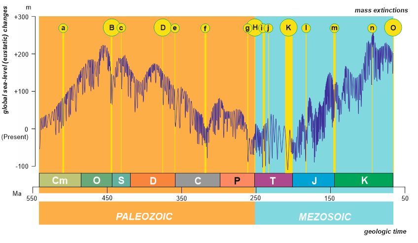
(Figure 2). Importantly,
transformative, stabilizing,mass extinctions
increasing, are also episodic
decreasing, events [38],
and interruptive which
events are always
(Figure negative
2). Importantly,
(biodiversity
mass extinctionsdrops)areand
alsoanomalous (very [38],
episodic events high which
extinction rate andnegative
are always outstanding biodiversity
(biodiversity drops).
drops) and
Although
anomalous some
(very(ifhigh
not all) mass extinctions
extinction were short-term
rate and outstanding events, and
biodiversity their duration
drops). Althoughwas someless(ifthan
not
that of theextinctions
all) mass consideredwere eustatic events,events,
short-term this is not
andtoo bigduration
their a limitation because
was less thanthisthatstudy
of theemphasizes
considered
the correspondence
eustatic events, this is of not mass
too bigextinctions
a limitation to eustatic
because this tendencies,
study emphasizes not particular, short-term
the correspondence of
fluctuations.
mass extinctions to eustatic tendencies, not particular, short-term fluctuations.
Classes of
Figure 2. Classes
Figure of episodic
episodic events
events (yellow
(yellow circles)
circles) that
that mark
mark changes
changes of
of eustatic
eustatic trends
trends (deep
(deep blue
lines) (modified
lines) (modified from
from[38]);
[38]);several
severalevents
eventsare
areshown
shownononthe
the same
same graphs
graphs to to illustrate
illustrate thethe variety
variety of
of situations.
situations.
Each eustatic event that happened within the occurrence of a given mass extinction is characterized
Each eustatic event that happened within the occurrence of a given mass extinction is
generally (i.e., as a global sea-level rise or fall, lowstand or highstand) and in relation to eustatic
characterized generally (i.e., as a global sea-level rise or fall, lowstand or highstand) and in relation
trends and their changes (regular or anomalous, ordinary or transformative, facilitative or stabilizing).
to eustatic trends and their changes (regular or anomalous, ordinary or transformative, facilitative or
Haq [32–34] and Haq and Schutter [35] outlined that their eustatic reconstructions allowed for the
stabilizing). Haq [32–34] and Haq and Schutter [35] outlined that their eustatic reconstructions
recognition of (at least) two orders of global sea-level changes that were provisionally labeled as
“short-term” and “long-term” changes. These orders are well visible in the joint curve employed for the
purposes of the present study (Figure 1). If so, it seems reasonable to also conduct the present analysis
of episodic events on two levels. The “short-term” record is limited to geologic epochs and periods, and
the “long-term” record corresponds to several geologic periods or eras. For instance, the “short-term”
trend is the global sea-level fall across the Silurian/Devonian transition, and the “long-term” trend
is the global sea-level rise during the Jurassic–Cretaceous. Biotic crises were geologically very short
events, but it cannot be excluded that they occurred due to biosphere vulnerability triggered by some
long-term processes.Life 2020, 10, 281 5 of 14
3. Results
From several biotic perturbations of the Cambrian, the end-Series 2 crisis deserves special attention
because of its strength [40,66,67]. This event corresponds to a pronounced eustatic fall followed by a
big rise, as depicted by Haq and Schutter [35]. However, this event was not anomalous, as similarly
strong fluctuations took place earlier and later during the Cambrian (Figure S1). The second half
of this period was characterized by the well-established “short-term” and “long-term” trends of the
global sea-level rise, and the event did not challenge these trends (Figure S1). Therefore, it was an
ordinary event.
A really severe mass extinction marked the end of the Ordovician, and it is known as the
Hirnantian event [41,42,68–70]. This biotic catastrophe corresponds to an outstanding eustatic fall
that was followed by a significant rise; the other fall of smaller magnitude, but reaching an even
lower negative peak, took place soon after the first fall [35]. Undoubtedly, both these falls were
anomalous relative to the preceding and subsequent events (Figure S1). In the “short-term” record,
the end-Ordovician eustatic event was evidently transformative, as it marked the change of the trend
(Figure S1). However, this event was interruptive in the “long-term” record because it broke the
general trend of the global sea-level fall that was established in the mid-Ordovician and ended in the
Permian, but this trend was restored soon after the end-Ordovician catastrophe (Figure S1).
A mass extinction took place at the Llandovery/Wenlock transition in the first half of the Silurian,
and it is known as the Ireviken event [43,71–74]. This event corresponds to a significant eustatic fall that
seems to be unusual for the Silurian, as depicted by Haq and Schutter [35]. Consequently, this event was
anomalous (Supplement 1). In the “short-term” record, this eustatic event was decreasing (Supplement
1). Its position relative to the “long-term” trend is less clear because this eustatic fall overlapped
with a longer, although relatively weak, eustatic lowstand already established in the Ordovician
(Supplement 1). This lowstand was evidently interruptive, but the role of the smaller lowstand at the
Llandovery/Wenlock transition is unclear, and it is provisionally defined as quasi-interruptive.
A significant mass extinction occurred at the Frasnian/Famennian transition in the Late Devonian,
and it is known as the Kellwasser event [44,75–78]. According to the reconstruction by Haq and
Schutter [35], this biotic catastrophe corresponds to relatively low-magnitude fluctuations of the global
sea level followed by a pronounced fall. This fall was anomalous in comparison to the other Devonian
eustatic changes, although similarly strong falls and rises became typical already in the second half of
the Late Devonian (Supplement 1). Notably, this event does not coincide with eustatic trend change
in the “short-term” and the “long-term” records (Supplement 1), and, thus, it looks like an ordinary
event. However, anomalous events cannot be ordinary by definition [38], and as such it is more correct
to classify this event as interruptive.
Another mid-Paleozoic mass extinction occurred at the Devonian/Carboniferous transition, and it
is known as the Hangenberg event [44,79–82]. This biotic catastrophe corresponds to a rather significant
global sea-level fall shown by Haq and Schutter [35]. The magnitude of this fall was unprecedented for
the Devonian, but not so uncommon for the following Mississippian Epoch (Supplement 1). Therefore,
the event can be classified as only relatively anomalous. In the “short-term” and “long-term” records,
it did not produce any principal change of the trends because the global sea level continued to fall
(Figure S1). This event is interruptive due to its relatively anomalous character.
There was a mass extinction near the end of the Mississippian, and this occurred in the late
Serpukhovian [45,46,83–85]. It corresponds to moderate eustatic fluctuations and preceded the
outstanding mid-Carboniferous eustatic minimum [35]. The noted fluctuations were typical for the
late Mississippian (Figure S1), and, thus, the event was regular. In the “short-term” record, this mass
extinction occurred when the global sea level tended to fall, but the intensity of this fall diminished
slightly (before the outstanding minimum that occurred later). Therefore, the eustatic event was
stabilizing. In the “long-term” record, this mass extinction coincided with a lengthy lowstand, which,
however, broke the general tendency of the global sea-level fall through the Middle–Late Paleozoic,
and as such the eustatic event is interruptive.Life 2020, 10, 281 6 of 14
A mass extinction that was a “prelude” to the end-Permian catastrophe occurred at the end of
the Guadalupian Epoch (Capitanian Stage) [47,48,86–88]. The timing of the event remains unclear,
and it is not excluded that it occurred earlier, i.e., in the mid-Capitanian [89,90]. In this study,
the very end-Guadalupian position of the catastrophe is considered, but this does not mean that the
forementioned alternative position is rejected. This mass extinction coincided with a significant eustatic
fall when the Paleozoic eustatic minimum was reached [35]. Undoubtedly, this event was anomalous
(Figure S1). In the “short-term” record, this fall was a stabilizing event, which marked the change
from the trend of the global sea-level fall from the mid-Permian to the relative stability during most
of the Lopingian, except at the very end (Figure S1). It is highly challenging to define this event in
the “long-term” record because the trends at the Paleozoic–Mesozoic transition are uncertain. Despite
the evident eustatic rises in the Early and Middle Triassic, the global sea level did not reveal a strong
tendency to rise until the beginning of the Jurassic (Figure S1). Therefore, it can be hypothesized that
the Triassic overall was a “long-term” lowstand established near the end of the Guadalupian. If so,
the end-Guadalupian eustatic fall was also a stabilizing event in the “long-term” record.
The most severe mass extinction stressed and almost “erased” the world marine biota at the
Permian/Triassic boundary [50,51,91–95]. This catastrophe corresponds to relatively weak eustatic
fluctuations as depicted by Haq and Schutter [35] and Haq [34]. There was a moderate global sea-level
rise followed by a similarly moderate fall; the magnitude of these changes was significantly smaller
than that of the preceding and subsequent fluctuations (Figure S1). Consequently, the event was
far from being anomalous. The larger global sea-level rises and falls that occurred just before and
just after the event were also regular. In the “short-term” record, the end-Permian mass extinction
coincided with the eustatic changes that marked an acceleration of the general trend of the global
sea-level rise (Figure S1). Consequently, a facilitative event can be postulated. In the “long-term”
record, the end-Permian mass extinction occurred soon after the start of the Lopingian–earliest Jurassic
lowstand and, therefore, the eustatic changes coinciding with this catastrophe can be classified as
ordinary, as they did not distort any trend.
In the Ladinian Stage of the Middle Triassic, the occurrence of a new mass extinction has
been argued recently [5,52]. Although this biotic perturbation still needs to be studied in detail,
its catastrophic nature has nonetheless been revealed. According to Haq [34], this mass extinction
corresponds to several eustatic fluctuations, from which the only global sea-level rise in the very
beginning was really significant. All these changes are rather typical for the Middle Triassic (Figure S1),
and, thus, these can be classified as regular. In both the “short-term” and “long-term” records, these
eustatic events did not challenge the trends (Figure S1) and are, therefore, ordinary.
The other extinction event occurred in the Carnian Stage of the Late Triassic [53]. This biotic
perturbation was reported very recently, but the arguments in favor of its existence are really strong.
According to Haq [34], this event corresponds to a strong eustatic fall. However, fluctuations of the
comparable magnitude were typical for the Late Triassic (Figure S1), and, thus, the noted fall is not
anomalous. Similarly to the previous biotic crisis, this fall did not change or disrupt “short-term” and
“long-term” trends (Figure S1), i.e., it was an ordinary event.
The next big mass extinction is known from the end-Triassic, and it occurred during most of
the Rhaetian Stage [54,55,96–100]. This biotic catastrophe corresponds to an outstanding global
sea-level fall followed by a similar rise and subsequent changes of lesser magnitude as depicted by
Haq [33,34] (Figure S1). Undoubtedly, the above fall and rise constitute an anomalous event. In the
“short-term” record, this event superimposed with the general tendency of the global sea-level fall that
was established in the beginning of the Late Triassic and culminated in the Early Jurassic (Figure S1),
i.e., this was an interruptive event. In the “long-term” record, this event occurred before the end of the
Lopingian–earliest Jurassic lowstand (Figure S1), i.e., it was interruptive relative to the general trend.
The Early Jurassic was marked by a mass extinction at the very beginning of the Toarcian
Stage [57–60,101–104]. This catastrophe corresponds to a significant global sea-level rise that was
followed by an even stronger fall [33]. This eustatic event is somewhat anomalous, although theLife 2020, 10, 281 7 of 14
magnitude of the Early–Middle Jurassic eustatic changes was relatively big (Figure S1). In the
“short-term” record, this event is marked by a trend change (Figure S1), and, thus, the event can
be classified as transformative. In the “long-term” record, this mass extinction coincided with a
pronounced lowstand superimposed on the Jurassic–Cretaceous trend of the global eustatic rise; after
this lowstand, the trend restarted from the lower point (Figure S1). This means this eustatic event
was decreasing.
The Jurassic/Cretaceous transition was marked by a mass extinction that, surprisingly, has been
studied significantly less than many other Mesozoic biotic perturbations [60,61]. This scant attention can
be explained partly by the still problematic stratigraphy of this transition interval (some improvements
have been made very recently [105–107]); a sensible and well-argued suggestion (although requiring
broad discussion before final approval) of the replacement of the period boundary has been made
recently [108], but even this solution will not allow us to correlate better the biodiversity losses and
turnovers at the planetary scale. According to the reconstruction by Haq [32,33], this mass extinction
corresponds to several eustatic fluctuations, the magnitude of which was comparable to that of many
other eustatic events of the latest Jurassic–earliest Cretaceous (Figure S1). Consequently, the noted
fluctuations were not anomalous. Taken together, the global sea-level changes at the mass extinction
interval constitute a particular composite event, i.e., a weak eustatic fall. This was also not an anomalous
event. In the “short-term” record, this composite event superimposed with the trend of global sea-level
fall established in the Late Jurassic and lasted until the mid-Early Cretaceous (Figure S1). If so, it was
an interruptive event. In the “long-term” record, this event marked the beginning of a lengthy break of
the Jurassic–Cretaceous trend of the global eustatic rise (Figure S1), i.e., this event was interruptive.
In the Late Cretaceous, a mass extinction occurred near the end of the Cenomanian Stage, which
is known as the Bonarelli event [62,63,103,109]. This biotic perturbation corresponds to small-scale
eustatic fluctuations that followed a very strong global sea-level rise [32]. The noted fluctuations
were very regular, and even the noted rise is difficult to classify as anomalous because fluctuations
of the same magnitude were typical for the entire first half of the Late Cretaceous (Figure S1). In the
“short-term” record, the eustatic rise at the onset of the mass extinction interval marked the change
from a trend of global sea-level fall to that of a rise (Figure S1), i.e., these events were transformative.
In the “long-term” record, attention should be paid to the small-magnitude fluctuations that occurred
just before the Cretaceous eustatic maximum, at which the Jurassic–Cretaceous trend of the eustatic rise
ended (Figure S1). With respect to this observation, the sea-level changes linked to the late Cenomanian
biotic catastrophe are transformative.
Finally, a severe and definitely the best-known mass extinction occurred in the very end of
the Cretaceous [65,110–115]. According to Haq [32], this catastrophe corresponds to a minor global
sea-level fall, which was a very regular event (Figure S1). In both the “short-term” and “long-term”
records, the event did not distort any trend, and as such it was ordinary. Even when expanding the
mass extinction interval so as to include the moderate-scale (relative to the other Late Cretaceous
events) fluctuation before the Cretaceous/Paleogene boundary (significant fall and significant rise—see
Supplement 1), this fluctuation is neither anomalous nor interruptive.
4. Discussion
Taking into account the most recent eustatic reconstructions [32–35] allows for realizing different
relationships between the Paleozoic–Mesozoic mass extinctions and the global sea-level changes
(Table 2). Although a falling sea level was found in more than half of the cases, the different eustatic
settings were not uncommon. Moreover, it is also evident that many biotic catastrophes occurred when
the eustatic changes were weak. Generally, no definitive relation can be found, and two inferences are
possible. First, even if eustatic changes were able to trigger mass extinctions, a eustatic cause can be
established only by a limited number of cases. In other words, this cause cannot represent a universal
explanation for all the mass extinction events. This interpretation echoes an earlier conclusion by
Hallam and Wignall [17] (Table 2). Therefore, improvements in both the eustatic reconstructions andLife 2020, 10, 281 8 of 14
the geologic time scale during the past 20 years did not make the eustatic cause of biodiversity losses
more plausible. Second, the global sea level and its changes determined environmental conditions in
which mass extinctions took place.
Table 2. Eustatic context of the considered mass extinctions.
Global Sea-Level Changes
Labels *
Hallam and Wignall [17] This Study
a not recorded strong fall and strong rise
B fall and rise strong falls with strong rise in between
c - strong fall
D rise weak fluctuations and strong fall
e rise strong fall
f - weak fluctuations
g fall strong fall
H rise weak fluctuations
i - strong rise and weak fluctuations
j - strong fall
K fall strong fall, strong rise, and weak fluctuations
l rise strong rise and strong fall
m - moderate fluctuations
n rise weak fluctuations and strong rise
O rise weak fall
Note: * see Figure 1 and Table 1.
The pioneering analysis of episodic events of eustatic changes provides somewhat ambiguous
evidence. On the one hand, many events were not anomalous (Table 3), i.e., the most relevant mass
extinctions occurred when the global sea-level did not experience extraordinary changes. This represents
strong evidence against the eustatic cause of many, if not all, mass extinctions. On the other hand,
the majority of the mass extinctions were linked to eustatic events that either interrupted or changed
the “short-term” and/or “long-term” trends of the global sea-level variations (Table 3). This evidence
seems to be enough to state that biotic catastrophes tended to associate with eustatic events that are not
ordinary. The results of the episodic event analysis do not permit us to neglect the potential importance
of eustatic changes to the mechanisms of mass extinctions. In light of the new findings, it is logical to
hypothesize that rather than global sea-level rises/falls, interruptions and changes of eustatic trends
could indeed facilitate or even trigger many Paleozoic–Mesozoic mass extinctions. Although the
full-argued explanation of the relevant mechanisms is yet to be developed, one can speculate that
interruptions of epoch-long and era-long tendencies of the global sea-level changes might be able to
stress marine communities via “putting” the latter into really new conditions that did not exist for a
long time before. Interrupted and changed trends created such new conditions. In order to illustrate
this idea, a simple, conceptual example can be given as follows. Marine biota evolved over a long
time in conditions of fluctuating, but generally rising, sea level, and its development was framed by
adaptation to the opening of new niches and increasing connectivity of water masses. If a trend of
sea-level fall was established later, this means marine biota needs adaptation to niche closure and
fragmentation of water masses. Indeed, these adaptations are developed, but this requires changes in
the ecosystem organization or distribution, which makes this biota vulnerable to negative external
influences and intrinsic factors during the transition from the past to modern conditions. Anyway,
this paper is not aimed at interpretations of the mechanisms beneath mass extinctions, although the
proposed framework for their relationships with sea-level changes might prove useful for further
interpretations of this issue.Life 2020, 10, 281 9 of 14
Table 3. Summary of the eustatic event interpretations linked to the considered mass extinctions.
Labels * Anomalous “Short-Term” Record “Long-Term” Record
a No ordinary ordinary
B Yes transformative interruptive
c Yes decreasing quasi-interruptive
D Yes interruptive interruptive
e Yes/No interruptive interruptive
f No stabilizing interruptive
g Yes stabilizing stabilizing
H No facilitative ordinary
i No ordinary ordinary
j No ordinary ordinary
K Yes interruptive interruptive
l Yes transformative decreasing
m No interruptive interruptive
n No transformative transformative
O No ordinary ordinary
Note: * see Figure 1 and Table 1.
The above-proposed hypothesis matters to the considered mass extinctions. One would wonder
whether all interruptions or changes of long- or short-term eustatic trends triggered biotic crises.
Definitely, this was not so. For instance, a trend change can be observed at the Carboniferous–Permian
transition (Figure 1), but the relevant transformative event is not associated with any mass extinction.
Some interruptions of a trend toward sea-level rise took place in the second half of the Jurassic, but
also without biotic crises. It should be stressed that interruptions and changes of eustatic trends were,
hypothetically, responsible for the vulnerable state of marine biota. In the absence of extrinsic or
intrinsic perturbations, this vulnerability may not lead to mass extinctions. In other words, interruptions
and changes of eustatic trends did not necessarily trigger biotic crises in the marine realm, but only
increased risks of negative scenarios.
5. Conclusions
The use of the new eustatic reconstructions by Haq [32–34] and Haq and Schutter [35] for the
understanding of the global sea-level changes at the intervals of the fifteen Paleozoic–Mesozoic mass
extinctions permits making two general conclusions. First, a direct relationship between the considered
biotic catastrophes in the marine realm and the eustatic rises/falls is absent. Second, many mass
extinctions correspond to interruptions and changes of the “short-term” and “long-term” eustatic trends.
Hypothetically, trend-affecting sea-level changes could facilitate or even trigger mass extinctions.
The explanatory mechanisms need to be well characterized, and this is a task for further investigations.
In other words, the outcomes of this study leave space for the eustatic explanation of biotic crises in
the marine realm, but indicate the urgency of changing the angle of looking at this factor.
Methodologically, the present paper demonstrates that the application of episodic event
analysis [38] provides a new vision of the eustatic factor of marine biota perturbations. Future
research may permit making the graphical analysis of trends more accurate (for instance, the trends
can be calculated as mathematical functions), and even classification of eustatic events with the power
of artificial intelligence may become possible. However, the solution of such an ambitious task requires
further refinement of the available eustatic curves. Moreover, better understanding of biotic crises,
their magnitude, and precise timing is desirable. For instance, the only very recent discovery of the
Carnian catastrophe [53] implies how incomplete the knowledge of mass extinctions can be even for
such well-studied geologic time intervals as the Mesozoic.
Supplementary Materials: The following are available online at http://www.mdpi.com/2075-1729/10/11/281/s1,
Figure S1: The Paleozoic-Mesozoic eustatic fluctuations, their trends, and mass extinctions (see text for more
information).Life 2020, 10, 281 10 of 14
Funding: This research received no external funding.
Acknowledgments: The author gratefully thanks the editorial team and the reviewers for their support and
helpful suggestions.
Conflicts of Interest: The author declares no conflict of interest.
References
1. Bambach, R.K. Phanerozoic biodiversity mass extinctions. Annu. Rev. Earth Planet. Sci. 2006, 34, 127–155.
[CrossRef]
2. Benton, M.J. The evolutionary significance of mass extinctions. Trends Ecol. Evol. 1986, 1, 127–130. [CrossRef]
3. Benton, M.J. Diversification and extinction in the history of life. Science 1995, 268, 52–58. [CrossRef]
4. Clapham, M.E.; Renne, P.R. Flood basalts and mass extinctions. Annu. Rev. Earth Planet. Sci. 2019, 47,
275–303. [CrossRef]
5. Elewa, A.M.T.; Abdelhady, A.A. Past, present, and future mass extinctions. J. Afr. Earth Sci. 2020, 162, 103678.
[CrossRef]
6. Erwin, D.H. The end and the beginning: Recoveries from mass extinctions. Trends Ecol. Evol. 1998, 13,
344–349. [CrossRef]
7. Hallam, A. Mass extinctions in Phanerozoic time. Geol. Soc. Spec. Publ. 1998, 140, 259–274. [CrossRef]
8. Holland, S.M. The Stratigraphy of Mass Extinctions and Recoveries. Annu. Rev. Earth Planet. Sci. 2020, 48,
75–97. [CrossRef]
9. Jablonski, D. Mass extinctions and macroevolution. Paleobiology 2005, 31, 192–210. [CrossRef]
10. Melott, A.L.; Bambach, R.K. Analysis of periodicity of extinction using the 2012 geological timescale.
Paleobiology 2014, 40, 177–196. [CrossRef]
11. Racki, G. The Alvarez impact theory of mass extinction; limits to its applicability and the “great expectations
syndrome”. Acta Palaeontol. Pol. 2012, 57, 681–702. [CrossRef]
12. Rampino, M.R.; Caldeira, K. Periodic impact cratering and extinction events over the last 260 million years.
Mon. Not. R. Astron. Soc. 2015, 454, 3480–3484. [CrossRef]
13. Raup, D.M.; Sepkoski, J.J., Jr. Mass extinctions in the marine fossil record. Science 1982, 215, 1501–1503.
[CrossRef] [PubMed]
14. Thomas, E. Cenozoic mass extinctions in the deep sea: What perturbs the largest habitat on Earth? Spec. Pap.
Geol. Soc. Am. 2004, 424, 1–23.
15. Twitchett, R.J. The palaeoclimatology, palaeoecology and palaeoenvironmental analysis of mass extinction
events. Palaeogeogr. Palaeoclimatol. Palaeoecol. 2006, 232, 190–213. [CrossRef]
16. Wignall, P.B. Large igneous provinces and mass extinctions. Earth-Sci. Rev. 2001, 53, 1–33. [CrossRef]
17. Hallam, A.; Wignall, P.B. Mass extinctions and sea-level changes. Earth Sci. Rev. 1999, 48, 217–250. [CrossRef]
18. Newell, N.D. Revolutions in the history of life. Geol. Soc. Am. Spec. Pap. 1967, 89, 63–91.
19. Peters, S.E.; Foote, M. Biodiversity in the Phanerozoic: A reinterpretation. Paleobiology 2001, 27, 583–600.
[CrossRef]
20. Roberts, G.G.; Mannion, P.D. Timing and periodicity of Phanerozoic marine biodiversity and environmental
change. Sci. Rep. 2019, 9, 6116. [CrossRef]
21. Smith, A.B. Large-scale heterogeneity of the fossil record: Implications for Phanerozoic biodiversity studies.
Philos. Trans. R. Soc. B Biol. Sci. 2001, 356, 351–367. [CrossRef] [PubMed]
22. Ruban, D.A. A “chaos” of Phanerozoic eustatic curves. J. Afr. Earth Sci. 2016, 116, 225–232. [CrossRef]
23. Ruban, D.A. Unawareness and Theorizing in Modern Geology: Two Examples Based on Citation Analysis.
Earth 2020, 1, 1–14. [CrossRef]
24. Raup, D.M.; Sepkoski, J.J., Jr. Periodicity of extinctions in the geologic past. Proc. Natl. Acad. Sci. USA 1984,
81, 801–805. [CrossRef]
25. Raup, D.M.; Sepkoski, J.J., Jr. Periodic extinction of families and genera. Science 1986, 231, 833–836. [CrossRef]
26. Boulila, S.; Laskar, J.; Haq, B.U.; Galbrun, B.; Hara, N. Long-term cyclicities in Phanerozoic sea-level
sedimentary record and their potential drivers. Glob. Planet. Chang. 2018, 165, 128–136. [CrossRef]
27. Gillman, M.P.; Erenler, H.E. Globally disruptive events show predictable timing patterns. Int. J. Astrobiol.
2016, 16, 91–96. [CrossRef]Life 2020, 10, 281 11 of 14
28. Lipowski, A. Periodicity of mass extinctions without an extraterrestrial cause. Phys. Rev. E Stat. Nonlinear
Soft Matter Phys. 2005, 71, 052902. [CrossRef]
29. McKinney, M.L. Periodic mass extinctions: Product of biosphere growth dynamics? Hist. Biol. 1989, 2,
273–287. [CrossRef]
30. Rampino, M.R. Relationship between impact-crater size and severity of related extinction episodes. Earth Sci.
Rev. 2020, 201, 102990. [CrossRef]
31. Tiwari, R.K.; Rao, K.N.N. Mega geocycles: Echoes of astronomical events. J. Geol. Soc. India 2003, 62, 181–190.
32. Haq, B.U. Cretaceous eustasy revisited. Glob. Planet. Chang. 2014, 113, 44–58. [CrossRef]
33. Haq, B.U. Jurassic sea-level variations: A reappraisal. Gsa Today 2018, 28, 4–10. [CrossRef]
34. Haq, B.U. Triassic eustatic variations reexamined. Gsa Today 2018, 28, 4–9. [CrossRef]
35. Haq, B.U.; Schutter, S.R. A chronology of Paleozoic sea-level changes. Science 2008, 322, 64–68. [CrossRef]
36. Haq, B.U.; Al-Qahtani, A.M. Phanerozoic cycles of sea-level change on the Arabian platform. GeoArabia 2005,
10, 127–160.
37. Haq, B.U.; Hardenbol, J.; Vail, P.R. Chronology of fluctuating sea levels since the Triassic. Science 1987, 235,
1156–1167. [CrossRef]
38. Ruban, D.A. Episodic events in long-term geological processes: A new classification and its applications.
Geosci. Front. 2018, 9, 377–389. [CrossRef]
39. International Commission on Stratigraphy (ICS). International Chronostratigraphic Chart, v2020/01. Available
online: https://stratigraphy.org/icschart/ChronostratChart2020-01.pdf (accessed on 15 October 2020).
40. Babcock, L.E.; Peng, S.-C.; Brett, C.E.; Zhu, M.-Y.; Ahlberg, P.; Bevis, M.; Robinson, R.A. Global climate, sea
level cycles, and biotic events in the Cambrian Period. Palaeoworld 2015, 24, 5–15. [CrossRef]
41. Ling, M.-X.; Zhan, R.-B.; Wang, G.-X.; Wang, Y.; Amelin, Y.; Tang, P.; Liu, J.-B.; Jin, J.; Huang, B.; Wu, R.-C.;
et al. An extremely brief end Ordovician mass extinction linked to abrupt onset of glaciation. Solid Earth Sci.
2020, 4, 190–198. [CrossRef]
42. Wang, G.; Zhan, R.; Percival, I.G. The end-Ordovician mass extinction: A single-pulse event? Earth Sci. Rev.
2019, 192, 15–33. [CrossRef]
43. Lehnert, O.; Männik, P.; Joachimski, M.M.; Calner, M.; Frýda, J. Palaeoclimate perturbations before the
Sheinwoodian glaciation: A trigger for extinctions during the ‘Ireviken Event’. Palaeogeogr. Palaeoclimatol.
Palaeoecol. 2010, 296, 320–331. [CrossRef]
44. Racki, G. A volcanic scenario for the Frasnian–Famennian major biotic crisis and other Late Devonian global
changes: More answers than questions? Glob. Planet. Chang. 2020, 189, 103174. [CrossRef]
45. Balseiro, D.; Powell, M.G. Carbonate collapse and the late Paleozoic ice age marine biodiversity crisis. Geology
2020, 48, 118–122. [CrossRef]
46. McGhee, G.R.; Clapham, M.E.; Sheehan, P.M.; Bottjer, D.J.; Droser, M.L. A new ecological-severity ranking of
major Phanerozoic biodiversity crises. Palaeogeogr. Palaeoclimatol. Palaeoecol. 2013, 370, 260–270. [CrossRef]
47. Arefifard, S.; Payne, J.L. End-Guadalupian extinction of larger fusulinids in central Iran and implications for
the global biotic crisis. Palaeogeogr. Palaeoclimatol. Palaeoecol. 2020, 550, 109743. [CrossRef]
48. Rampino, M.R.; Shen, S.-Z. The end-Guadalupian (259.8 Ma) biodiversity crisis: The sixth major mass
extinction? Hist. Biol. 2019. [CrossRef]
49. Rampino, M.R.; Eshet-Alkalai, Y.; Koutavas, A.; Rodriguez, S. End-Permian stratigraphic timeline applied to
the timing of marine and non-marine extinctions. Palaeoworld 2020, 29, 577–589. [CrossRef]
50. Shen, S.-Z.; Ramezani, J.; Chen, J.; Cao, C.-Q.; Erwin, D.H.; Zhang, H.; Xiang, L.; Schoepfer, S.D.; Henderson, C.M.;
Zheng, Q.-F.; et al. A sudden end-Permian mass extinction in South China. Bull. Geol. Soc. Am. 2019, 131,
205–223. [CrossRef]
51. Song, H.; Wignall, P.B.; Tong, J.; Yin, H. Two pulses of extinction during the Permian-Triassic crisis. Nat. Geosci.
2013, 6, 52–56. [CrossRef]
52. Ruban, D.A. Examining the Ladinian crisis in light of the current knowledge of the Triassic biodiversity
changes. Gondwana Res. 2017, 48, 285–291. [CrossRef]
53. Dal Corso, J.; Bernardi, M.; Sun, Y.; Song, H.; Seyfullah, L.J.; Preto, N.; Gianolla, P.; Ruffell, A.; Kustatscher, E.;
Roghi, G.; et al. Extinction and dawn of the modern world in the Carnian (Late Triassic). Sci. Adv. 2020, 6,
eaba0099. [CrossRef] [PubMed]Life 2020, 10, 281 12 of 14
54. Rigo, M.; Onoue, T.; Tanner, L.H.; Lucas, S.G.; Godfrey, L.; Katz, M.E.; Zaffani, M.; Grice, K.; Cesar, J.;
Yamashita, D.; et al. The Late Triassic Extinction at the Norian/Rhaetian boundary: Biotic evidence and
geochemical signature. Earth Sci. Rev. 2020, 204, 103180. [CrossRef]
55. Tegner, C.; Marzoli, A.; McDonald, I.; Youbi, N.; Lindström, S. Platinum-group elements link the end-Triassic
mass extinction and the Central Atlantic Magmatic Province. Sci. Rep. 2020, 10, 3482. [CrossRef]
56. Wignall, P.B.; Atkinson, J.W. A two-phase end-Triassic mass extinction. Earth Sci. Rev. 2020, 208, 103282.
[CrossRef]
57. Ait-Itto, F.-Z.; Martinez, M.; Price, G.D.; Ait Addi, A. Synchronization of the astronomical time scales
in the Early Toarcian: A link between anoxia, carbon-cycle perturbation, mass extinction and volcanism.
Earth Planet. Sci. Lett. 2018, 493, 1–11. [CrossRef]
58. Caruthers, A.H.; Smith, P.L.; Gröcke, D.R. The Pliensbachian-Toarcian (Early Jurassic) extinction: A North
American perspective. Spec. Pap. Geol. Soc. Am. 2014, 505, 225–243.
59. Ruebsam, W.; Reolid, M.; Marok, A.; Schwark, L. Drivers of benthic extinction during the early Toarcian
(Early Jurassic) at the northern Gondwana paleomargin: Implications for paleoceanographic conditions.
Earth Sci. Rev. 2020, 203, 103117. [CrossRef]
60. Hallam, A. The Pliensbachian and Tithonian extinction events. Nature 1986, 319, 765–768. [CrossRef]
61. Ruban, D.A. Diversity dynamics of Callovian-Albian brachiopods in the Northern Caucasus (Northern
Neo-Tethys) and a Jurassic/Cretaceous mass extinction. Paleontol. Res. 2011, 15, 154–167. [CrossRef]
62. Freymueller, N.A.; Moore, J.R.; Myers, C.E. An analysis of the impacts of Cretaceous oceanic anoxic events
on global molluscan diversity dynamics. Paleobiology 2019, 45, 280–295. [CrossRef]
63. Hart, M.B. The ’Black Band’: Local expression of a global event. Proc. Yorks. Geol. Soc. 2018, 62, 217–226.
[CrossRef]
64. Kuroda, J.; Ogawa, N.O.; Tanimizu, M.; Coffin, M.F.; Tokuyama, H.; Kitazato, H.; Ohkouchi, N.
Contemporaneous massive subaerial volcanism and late cretaceous Oceanic Anoxic Event 2. Earth Planet.
Sci. Lett. 2007, 256, 211–223. [CrossRef]
65. Schoene, B.; Eddy, M.P.; Samperton, K.M.; Keller, C.B.; Keller, G.; Adatte, T.; Khadri, S.F.R. U-Pb constraints
on pulsed eruption of the Deccan Traps across the end-Cretaceous mass extinction. Science 2019, 363, 862–866.
[CrossRef]
66. Faggetter, L.E.; Wignall, P.B.; Pruss, S.B.; Newton, R.J.; Sun, Y.; Crowley, S.F. Trilobite extinctions, facies
changes and the ROECE carbon isotope excursion at the Cambrian Series 2–3 boundary, Great Basin, western
USA. Palaeogeogr. Palaeoclimatol. Palaeoecol. 2017, 478, 53–66. [CrossRef]
67. Guo, Q.; Strauss, H.; Liu, C.; Zhao, Y.; Yang, X.; Peng, J.; Yang, H. A negative carbon isotope excursion
defines the boundary from Cambrian Series 2 to Cambrian Series 3 on the Yangtze Platform, South China.
Palaeogeogr. Palaeoclimatol. Palaeoecol. 2010, 285, 143–151. [CrossRef]
68. Brenchley, P.J.; Carden, G.A.F.; Marshall, J.D. Environmental changes associated with the "first strike’ of the
late Ordovician mass extinction. Mod. Geol. 1995, 20, 69–82.
69. Sheehan, P.M. The late Ordovician mass-extinction. Annu. Rev. Earth Planet. Sci. 2001, 29, 331–364. [CrossRef]
70. Sutcliffe, O.E.; Dowdeswell, J.A.; Whittington, R.J.; Theron, J.N.; Craig, J. Calibrating the Late Ordovician
glaciation and mass extinction by the eccentricity cycles of Earth’s orbit. Geology 2000, 28, 967–970. [CrossRef]
71. Eriksson, M.E. The Silurian Ireviken Event and vagile benthic faunal turnovers (Polychaeta; Eunicida) on
Gotland, Sweden. GFF 2006, 128, 91–95. [CrossRef]
72. Jeppsson, L.; Aldridge, R.J.; Dorning, K.J. Wenlock (Silurian) oceanic episodes and events. J. Geol. Soc. 1995,
152, 487–498. [CrossRef]
73. Johnson, M.E. Relationship of Silurian sea-level fluctuations to oceanic episodes and events. GFF 2006, 128,
115–121. [CrossRef]
74. Munnecke, A.; Samtleben, C.; Bickert, T. The Ireviken Event in the lower Silurian of Gotland,
Sweden—Relation to similar Palaeozoic and Proterozoic events. Palaeogeogr. Palaeoclimatol. Palaeoecol. 2003,
195, 99–124. [CrossRef]
75. Bond, D.P.G.; Wignall, P.B. The role of sea-level change and marine anoxia in the Frasnian-Famennian (Late
Devonian) mass extinction. Palaeogeogr. Palaeoclimatol. Palaeoecol. 2008, 263, 107–118. [CrossRef]
76. McGhee, G.R. The Late Devonian (Frasnian/Famenian) mass extinction: A proposed test of the glaciation
hypothesis. Geol. Q. 2014, 58, 263–268. [CrossRef]Life 2020, 10, 281 13 of 14
77. De Vleeschouwer, D.; Da Silva, A.-C.; Sinnesael, M.; Chen, D.; Day, J.E.; Whalen, M.T.; Guo, Z.; Claeys, P.
Timing and pacing of the Late Devonian mass extinction event regulated by eccentricity and obliquity.
Nat. Commun. 2017, 8, 2268. [CrossRef]
78. Sandberg, C.A.; Morrow, J.R.; Ziegler, W. Late Devonian sea-level changes, catastrophic events, and mass
extinctions. Spec. Pap. Geol. Soc. Am. 2002, 356, 473–487.
79. Becker, R.T.; Kaiser, S.I.; Aretz, M. Review of chrono-, litho- and biostratigraphy across the global Hangenberg
Crisis and Devonian-Carboniferous Boundary. Geol. Soc. Spec. Publ. 2016, 423, 355–386. [CrossRef]
80. Kaiser, S.I.; Aretz, M.; Becker, R.T. The global Hangenberg Crisis (Devonian-Carboniferous transition):
Review of a first-order mass extinction. Geol. Soc. Spec. Publ. 2016, 423, 387–437. [CrossRef]
81. Matyja, H.; Sobien, K.; Marynowski, L.; Stempien-Salek, M.; Malkowski, K. The expression of the Hangenberg
Event (latest Devonian) in a relatively shallow-marine succession (Pomeranian Basin, Poland): The results of
a multi-proxy investigation. Geol. Mag. 2015, 152, 400–428. [CrossRef]
82. Myrow, P.M.; Ramezani, J.; Hanson, A.E.; Bowring, S.A.; Racki, G.; Rakocinski, M. High-precision U-Pb age
and duration of the latest Devonian (Famennian) hangenberg event, and its implications. Terra Nova 2014, 26,
222–229. [CrossRef]
83. Cózar, P.; Vachard, D.; Somerville, I.D.; Medina-Varea, P.; Rodríguez, S.; Said, I. The Tindouf Basin, a marine
refuge during the Serpukhovian (Carboniferous) mass extinction in the northwestern Gondwana platform.
Palaeogeogr. Palaeoclimatol. Palaeoecol. 2014, 394, 12–28. [CrossRef]
84. Kelley, P.H.; Raymond, A. Migration, origination and extinction of Southern Hemisphere brachiopods during
the middle Carboniferous. Palaeogeogr. Palaeoclimatol. Palaeoecol. 1991, 86, 23–39. [CrossRef]
85. Raymond, A.; Kelley, P.H.; Blanton Lutken, C. Dead by degrees: Articulate brachiopods, paleoclimate and
the Mid- Carboniferous extinction event. Palaios 1990, 5, 111–123. [CrossRef]
86. Ali, J.R.; Thompson, G.M.; Song, X.; Wang, Y. Emeishan Basalts (SW China) and the ’end-Guadalupian’ crisis:
Magnetobiostratigraphic constraints. J. Geol. Soc. 2002, 159, 21–29. [CrossRef]
87. Clapham, M.E.; Shen, S.; Bottjer, D.J. The double mass extinction revisited: Reassessing the severity, selectivity,
and causes of the end-Guadalupian biotic crisis (Late Permian). Paleobiology 2009, 35, 32–50. [CrossRef]
88. Zhou, M.-F.; Malpas, J.; Song, X.-Y.; Robinson, P.T.; Sun, M.; Kennedy, A.K.; Lesher, C.; Keays, R.R. A temporal
link between the Emeishan large igneous province (SW China) and the end-Guadalupian mass extinction.
Earth Planet. Sci. Lett. 2002, 196, 113–122. [CrossRef]
89. Zhang, B.; Yao, S.; Hu, W.; Ding, H.; Liu, B.; Ren, Y. Development of a high-productivity and anoxic-euxinic
condition during the late Guadalupian in the Lower Yangtze region: Implications for the mid-Capitanian
extinction event. Palaeogeogr. Palaeoclimatol. Palaeoecol. 2019, 531, 108630. [CrossRef]
90. Zhang, B.; Wignall, P.B.; Hu, W.; Liu, B.; Ren, Y. New timing and geochemical constraints on the capitanian
(Middle permian) extinction and environmental changes in deep-water settings: Evidence from the lower
yangtze region of South China. J. Geol. Soc. 2019, 176, 588–608. [CrossRef]
91. Benton, M.J.; Twitchett, R.J. How to kill (almost) all life: The end-Permian extinction event. Trends Ecol. Evol.
2003, 18, 358–365. [CrossRef]
92. Erwin, D.H.; Bowring, S.A.; Yugan, J. End-Permian mass extinctions: A review. Spec. Pap. Geol. Soc. Am.
2002, 356, 363–383.
93. Knoll, A.H.; Bambach, R.K.; Canfield, D.E.; Grotzinger, J.P. Comparative earth history and late Permian mass
extinction. Science 1996, 273, 452–457. [CrossRef] [PubMed]
94. Shen, S.-Z.; Crowley, J.L.; Wang, Y.; Bowring, S.A.; Erwin, D.H.; Sadler, P.M.; Cao, C.-Q.; Rothman, D.H.;
Henderson, C.M.; Ramezani, J.; et al. Calibrating the end-Permian mass extinction. Science 2011, 334,
1367–1372. [CrossRef] [PubMed]
95. Wignall, P.B.; Twitchett, R.J. Oceanic anoxia and the end Permian mass extinction. Science 1996, 272, 1155–1158.
[CrossRef] [PubMed]
96. Deenen, M.H.L.; Ruhl, M.; Bonis, N.R.; Krijgsman, W.; Kuerschner, W.M.; Reitsma, M.; van Bergen, M.J.
A new chronology for the end-Triassic mass extinction. Earth Planet. Sci. Lett. 2010, 291, 113–125. [CrossRef]
97. Hallam, A. How catastrophic was the end-Triassic mass extinction? Lethaia 2002, 35, 147–157. [CrossRef]
98. Pálfy, J.; Mortensen, J.K.; Carter, E.S.; Smith, P.L.; Friedman, R.M.; Tipper, H.W. Timing the end-Triassic mass
extinction: First on land, then in the sea? Geology 2000, 28, 39–42. [CrossRef]
99. Schoene, B.; Guex, J.; Bartolini, A.; Schaltegger, U.; Blackburn, T.J. Correlating the end-Triassic mass extinction
and flood basalt volcanism at the 100 ka level. Geology 2010, 38, 387–390. [CrossRef]You can also read