PANDA: Placement of Unmanned Aerial Vehicles Achieving 3D Directional Coverage
←
→
Page content transcription
If your browser does not render page correctly, please read the page content below
PANDA: Placement of Unmanned Aerial Vehicles
      Achieving 3D Directional Coverage
    Weijun Wang∗ Haipeng Dai∗ Chao Dong† Xiao Cheng∗ Xiaoyu Wang∗ Guihai Chen∗ Wanchun Dou∗
          ∗
          State Key Laboratory for Novel Software Technology, Nanjing University, Nanjing, Jiangsu 210024, CHINA
                   †
                     Nanjing University of Aeronautics and Astronautics, Nanjing, Jiangsu 210007, CHINA
Emails: {haipengdai, gchen, wcdou}@nju.edu.cn, dch999@gmail.com, {weijunwang, xiaocheng, xiaoyuwang}@smail.nju.edu.cn


   Abstract—This paper considers the fundamental problem of


Placement of unmanned Aerial vehicles achieviNg 3D Directional

coverAge (PANDA), that is, given a set of objects with determined
positions and orientations in a 3D space, deploy a fixed number of
UAVs by adjusting their positions and orientations such that the
overall directional coverage utility for all objects is maximized.

First, we establish the 3D directional coverage model for both
cameras and objects. Then, we propose a Dominating Coverage

Set (DCS) extraction method to reduce the infinite solution space                Fig. 1: 3D Directional coverage model
of PANDA to a limited one without performance loss. Finally,
we model the reformulated problem as maximizing a monotone
submodular function subject to a matroid constraint, and present     recognition [23] UAVs won’t be more than 15m far and
a greedy algorithm with 1 − 1/e approximation ratio to address       5m high from the human faces, which implies the height of
this problem. We conduct simulations and field experiments to         humans cannot be ignored, especially they are on different
evaluate the proposed algorithm, and the results show that our       floors. Another example, in crop inspection [24] UAVs need
algorithm outperforms comparison ones by at least 75.4%.
                                                                     to monitor crop closely to capture the details of them, hence
                                                                     the height of crop also cannot be neglected.
                      I. I NTRODUCTION
                                                                        In this paper, we study the problem of Placement of Un-
   Camera sensor network has attracted great attention in            manned Aerial Vehicles achieviNg 3D Directional coverAge
recent years as it provides detailed data of environment by          (PANDA). In our considered scenario, some objects are dis-
retrieving rich information in the form of images and videos         tributed in 3D space with known facing direction, and we
[1], [2]. It has found a wide range of applications, such as         have a given number of UAVs to deploy in the free 3D space
surveillance, traffic monitoring, and crowd protection, etc.          whose cameras can freely adjust their orientation. The practical
For some temporary situations, such as assembly, concerts,           3D directional coverage model for cameras and objects is
matches, and outdoor speeches, establishing stationary camera        established as Figure 1. The coverage space of camera is
sensor network in advance may cost too much time and money,          modeled as a straight rectangle pyramid and the efficient
and may be inconvenient or even impossible. Fortunately, the         coverage space of object is modeled as a spherical base
development of Unmanned Aerial Vehicle (UAV) technology              cone, which are both fundamentally different from previous
in the past few years [3], [4] offers a promising way to address     work. Moreover, we define directional coverage utility to
this issue. With the low-cost and agile UAVs, camera sensor          characterize the effectiveness of directional coverage for all
network can be deployed dynamically to capture real-time,            objects. Formally, given a fixed number of UAVs and a set
reliable and high-quality images and videos. For example, DJI        of objects in the space, PANDA problem is to deploy the
Phantom 4 UAV can fly at 72 km/h, rise at 6 m/s, swerve at            UAVs in the 3D free space, i.e., to determine their coordinates
250 ◦ /s, and provide 2K real-time images and videos [5].            and orientations (the combinations of which we define as
   To guarantee high quality of monitoring, UAVs should              strategies), such that the directional coverage utility for all
jointly adjust their coordinates and the orientations of their       objects is maximized.
cameras to cover objects at or near their frontal view [6].             We face two main technical challenges to address PANDA.
Though some sensor placement methods have emerged to                 The first challenge is that the problem is essentially continues
study directional sensor or camera sensor coverage problem           and nonlinear. The problem is continues because both coor-
[7]–[19], none of them considers that sensors and objects are        dinates and orientations of UAVs are continuous values. It is
placed in 3D environment. Although a few camera sensor               also nonlinear because the angular constraints for both camera
coverage methods consider 3D environment [20]–[22], almost           model and object model, and the constraint of pitching angle
all of them assume that all objects are still distributed on         of camera in objective function. The second challenge is to
2D plane. However, in many scenarios, the objects cannot             develop an approximation algorithm which needs to bound
be served as distributed on 2D plane. For example, in face           the performance gap to the optimal solution.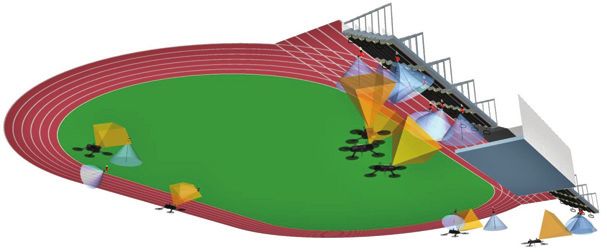
To address these two challenges, first, we propose a Domi-                                                        TABLE I: Notations
nating Coverage Set extraction method to reduce the continu-                   Symbol            Meaning
ous search space of strategies of UAVs to a limited number of                        ci          UAV i, or its 3D coordinate
strategies without performance loss. Hence, PANDA problem                            oj          Object j to be monitored, or its 3D coordinate
                                                                                     N           Number of UAVs to be deployed
becomes to select a fixed number of strategies from a set                            M            Number of objects to be monitored
of candidate ones to maximize the overall object directional                       dci          Orientation of camera of UAV i
coverage utility, which is discrete, and we address the first                          γ          Pitching angle of camera
challenge. Then, we prove that the reformulated problem falls                   γmin             Minimum pitching angle
                                                                                γmax             Maximum pitching angle
into the scope of the problem of maximizing a monotone
                                                                                      α          Horizontal offset angles of the FoV around dci
submodular function subject to a matroid constraint, which                            β          Vertical offset angles of the FoV around dci
allows a greedy algorithm to achieve a constant approximation                     doj           Orientation of object oj
ratio. Consequently, we address the second challenge.                                 θ          Efficient angle around doj for directional coverage
                                                                                     D           Farthest sight distance of camera with guaranteed moni-
                    II. R ELATED W ORKS                                                          toring quality
   Directional sensor coverage and camera sensor coverage.

Directional sensor coverage works can be classified into object


coverage and area coverage, whose respective goal is maximiz-


ing the number of covered objects [7], [25] and area coverage

ratio [8], [26], but most of them do not take the objects’ facing
direction into account [10]. In addition, although most of


camera sensor coverage works consider objects’ facing direc-

tion [9], [27], [28] and address directional coverage problems
                                                                           Fig. 2: Camera model                                     Fig. 3: Directional coverage
under various scenarios, i.e., barrier coverage [27], they only
                                                                                                                                    model
consider 2D sector model which is also the assumption of most
of directional sensor coverage works.
   3D camera sensor coverage. There exists a few works              to face any horizonal orientation. By a little abuse of notation,
focusing on camera sensor coverage in 3D environment. Ma            ci and oj also denote the coordinate of UAV and object. Table
et al. in [20] proposed the first 3D camera coverage model           I lists the notations we use in this paper.
and developed an algorithm for area coverage on 2D plane
                                                                    A. Camera Model
with the projecting quadrilateral area of 3D camera coverage
model. Based on this model, Yang et al. in [29] introduced             More complicated than previous sector model of 2D direc-
coverage correlation model of neighbor cameras to decrease          tional sensor, camera model in 3D environment needs to be
the number of cameras. Han et al. in [30] and Yang et               modeled as a straight rectangular pyramid as shown in Figure
al. in [31] took energy and storage of camera sensors into          2. Due to cameras only can rotate in vertical plane, edge AC
account and proposed high-efficient resource utility coverage        and BD are always parallel to the ground.
algorithm. Si et al. in [32] considered the intruders’ facing          We use a 5-tuple (ci , dci , γ, α, β) to denote the cam-
direction and the size of face in barrier coverage. Hosseini        era model. As illustrated in Figure 2, point ci denotes the
et al. in [33] addressed the problem of camera selection and        coordinate of UAV ci , its value is (x0 , y0 , z0 ). Vector dci
configuration problem for object coverage by binary integer          denotes the orientation of ci ’s camera which is perpendic-
programming solution. Li et al. in [21] and Peng et al. in [22],    ular to undersurface ABCD and its unit vector equals to
[34] established a more practical 3D camera coverage model,         (x1 , y1 , z1 ). Point O is the centre of rectangle ABCD and
and studied three area coverage problems based on this model.       the distance |ci O| = D, where D is the farthest distance
However, most of above works simply use 3D camera coverage          from camera which can guarantee the quality of monitoring
model to address those problems whose covered objects or            of every object on ABCD. Thus, the coordinate of point O is
area are only distributed on 2D plane, and thus none of them        (x0 + Dx1 , y0 + Dy1 , z0 + Dz1 ). Clearly, we can mathematically
can solve our problem.                                              express plane ABCD as
                                                                                                                 ⎛            ⎞
                 III. P ROBLEM S TATEMENT                                                                     x − (x0 + Dx1 )
                                                                                                            ⎜                 ⎟
                                                                                                     dci · ⎝ y − (y0 + Dy1 ) ⎠ = 0.                           (1)
   Suppose we have M objects O = {o1 , o2 , ..., oM } to be
monitored in a 3D free space, each object oj has a known                                                      z − (z0 + Dz1 )
orientation, which is denoted by a vector doj . We also have
                                                                       Connecting point ci to midpoint P of AC and Q of CD
N UAVs C = {c1 , c2 , ..., cN } equipped with cameras which
                                                                    respectively, we can get plane ci OP and ci OQ. As cameras
can hover anywhere in the 3D free space. Because of hardware
                                                                    only can rotate in vertical field, plane ci OP is parallel to z-
limitation, their cameras can only rotate in the vertical plane.
                                                                    axis. Thus, plane ci OP can be expressed as
However, this limitation has no influence to the coverage
orientation, because UAV can hover in the air and rotate itself                                      −y1 x + x1 y + x0 y1 − y0 x1 = 0.                         (2)
As shown in Figure 2, OQ ⊥ OP , OQ ⊥ Oci , thus OQ ⊥ Then, the directional coverage utility can be defined as
ci OP . By Equation (2) and ∠Oci Q equals to the horizontal 1, N
Fv (ci , oj , dci , doj ) ≥ 1,
offset angle α, so |OQ| = D · tan α . Thus, we can obtain Uv (ci , dci , oj , doj ) = i=1
(8)
0, otherwise.
−−
→
OQ = D · tan α · (−y1 , x1 , 0). (3)
C. Problem Formulation
Similar, OP ⊥ ci OQ, ∠Oci P equals to the vertical offset Let the tuple ci , dci , called strategy, denotes the coordi-
angle β, then we have |OP | = D ·tan β . Combine the equation nate of UAV ci and orientation of its camera dci . Due to the
−−→
of plane ci OP , vector OP can be obtained as limited resource of UAV, our task is to determine the strategies
−
−→
OP = (x1 z1 , y1 z1 , −y12 − x21 ) · D · tan β. (4) for all N UAVs to optimize overall directional coverage utility
for all M objects, namely the number of directional covered
To a given object oj , if oj is covered by ci , it must be in objects. Formally, the PANDA problem is defined as follows.
some rectangle which is parallel to ABCD, i.e. rectangle Ω
M
N
between ci and ABCD in Figure 2. According to this idea, (P1) max Uv ( Fv (ci , oj , dci , doj )),
we can illustrate the camera model as follows. Point O is j=1 i=1
the centre of the rectangle and its coordinate is easy to figure s.t. γmin ≤ γ ≤ γmax .
−−→
out by oj and normal vector dci . Utilize normal vectors OQ Since the function Fv (·) is nonlinear and the constraints
−−→
in Equation (3) and OP in Equation (4), if oj satisfies the of P1 is continuous, PANDA falls in the realm of nonlinear
following constraint, point oj is covered by camera ci . programs which are NP-hard [35]. Hence, we have
⎧
Theorem 3.1: The PANDA problem is NP-hard.
−−→
⎪
⎪ 1, P rj−
−→ O oj ≤ |O P |,
⎪
⎪
OP IV. S OLUTION
⎪
⎨ −−→
P rj−
−→ O oj ≤ |O Q |,
Fc (ci ,oj , dci , doj ) = OQ In this section, we present an algorithm with approximation
⎪
⎪
⎪ P rj − c−→
o ≤ D.
ci i j ratio 1 − 1/e to address PANDA. Before describing the details
⎪
⎪
d
(5)
⎩0, otherwise. of it, we first present the key intuitions and solution overview.
s.t. |ci O | = P rjdci −
c−→
i oj , |O P | = |ci O | · tan β,
A. Key Intuitions and Solution Overview
|O Q | = |ci O | · tan α. 1) Key Intuitions: (1) Focus on possible covered sets of
objects of UAVs rather than candidate positions and orienta-
B. 3D Directional Coverage Model tions of UAVs. As we can deploy UAVs on any position and
First, we define 3D directional coverage as follows. set the orientation of their cameras arbitrarily, the number of
Definition 3.1: (3D directional coverage) For an given candidate strategies of UAVs is infinite, or the solution space
object oj and its facing direction d(x, y, z), there is an UAV of PANDA is infinite. However, many strategies are essentially
ci with camera orientation dci , such that oj is covered by ci equivalent if they cover the same set of objects. Apparently, we
and α(d,−o−→
j ci ) ≤ θ (θ is called the efficient angle), then object
only need to consider one representative strategy among its as-
oj is 3D directional covered by ci . sociated class of all equivalent strategies, and the number of all
According to Definition 3.1, object model can be established such representative strategies is finite because the number of
as a spherical base cone as Figure 3. Let Object oj be the all possible covered sets of objects is finite. (2) Focus on those
vertex, rotate a sector of θ central angle and D radius around strategies that cover large sets of objects. If a representative
vector d for one revolution, then we obtain the object model strategy covers the set of objects {o1 , o2 , o3 , o4 }, undoubtedly
as follows. you don’t need to consider strategies that cover its subsets,
−−→ |ci oj | ≤ D, such as {o1 , o2 } or {o2 , o3 , o4 }. Our goal is to find those
(6)
α(o−−→
j ci , doj ) ≤ θ.
representative strategies that possibly cover maximal covered
sets of objects while avoiding the others. (3) Find or “create”
Based on Equation (6), UAV ci can efficiently cover object
constraints to help determine representative strategies. To
oj only when it locates in the cone of object oj where can
uniquely determine a strategy, mathematically we need at least
guarantee |−c−→ −−→
i oj | ≤ D and α(oj ci , doj ) ≤ θ . Thereby, combine
9 equations. Then, even if we know the associated covered
Equation (5) and (6), we can obtain the directional coverage
set of objects for a class of equivalent strategies how can
function as ⎧ −−→ we efficiently determine at least one representative strategy?
⎪
⎪ 1, P rj−
−→ O oj ≤ |O P |,
⎪
⎪ OP Our solution is to imagine that given a feasible strategy,
⎪
⎪ −−→
⎪
⎪ P rj−
−→ O oj ≤ |O Q |, we can adjust its position and orientation such that one or
⎨ OQ
Fv (ci ,oj , dci , doj ) =
⎪ P rj − c−→
o ≤ |−
ci i j c−→
o | ≤ D.
i j
more objects touch some sides of the pyramid of the strategy
⎪
⎪
d
while keeping no objects out of coverage. Obviously, the
⎪
⎪
⎪ α(−
o−→
j ci , doj ) ≤ θ.
(7)
⎪
⎪ obtained strategy after the adjustment is also feasible and
⎩
0, otherwise can be selected as a representative strategy. Then, we in turn
s.t. |ci O | = P rjdci ci→
−−oj , |O P | = |ci O | × tan β, use the touching conditions as constraints and formulate them
|O Q | = |ci O | · tan α. as equations to help determine the representative strategies.Apart from such kind of constraints, we also find an additional
constraint regarding positions of representative strategies for C. Dominating Coverage Set (DCS) Extraction
their determination in this paper. After the space partition, we only need to consider the
2) Solution Overview: First, any object only can be ef- relationship between objects and UAVs in each subspace,
ficinetly covered by an UAV in its efficient coverage space, which depends on the coordinates and orientations of UAVs.
which is modeled as a spherical base cone, by the 3D In this subsection, we show that instead of enumerating all
Directional Coverage Model. The whole solution space is possible covered sets of objects, we only need to consider
thus the union of all spherical base cones for all objects. a limited number of representative covered sets of objects,
We further present a space partition approach to partition the which are defined as Dominating Coverage Sets (DCSs), and
whole solution space into multiple subspaces, which can be figure out their corresponding strategies. Our ultimate goal is
considered separately. Especially, for each subspace, the set of to reduce the problem to a combinatorial optimization problem
all possibly covered objects by adjusting the orientation of an which is selecting N strategies from a limited number of
UAV at any point in the subspace is exactly the same. strategies obtained by DCS extraction.
Second, we propose the notion of Dominating Coverage 1) Preliminaries: To begin with, we give the following
Set (DCS), which covers the maximal set of objects and has definitions to assist analysis.
no proper superset of covered objects by other strategies. Definition 4.1: (Dominance) Given two strategies c1 , dc1 ,
Then, our goal turns to find all candidate DCSs and their c2 , dc2 and their covered sets of objects O1 and O2 . If
associated representative strategies. Specifically, we first prove O1 = O2 , c1 , dc1 is equivalent to c2 , dc2 , or c1 , dc1
that the positions of associated strategies of DCSs must lie on ≡ c2 , dc2 ; If O1 ⊃ O2 , c1 , dc1 dominates c2 , dc2 , or
the boundaries of subspaces, which serves as a constraint to c1 , dc1 c2 , dc2 ; And if O1 ⊇ O2 , c1 , dc1 c2 , dc2 .
help determine the representative strategies. Next, we imagine Definition 4.2: (Dominating Coverage Set) Given a set of
that we adjust the positions and orientations of strategies to objects Oi covered by a strategy ci , dci , if there does not
create touching conditions and thus new constraints. More exist a strategy cj , dcj such that cj , dcj ci , dci , then
importantly, we prove that it is sufficient to enumerate the Oi is a Dominating Coverage Set (DCS).
seven different cases where 1 to 7 objects touch on the For a given subspace, it is possible only a few objects in
sides of pyramid in order to extract all possible DCSs, and the ground set of objects can be covered by an UAV locating
the enumeration process must be done in polynomial time. in this subspace. We formally give the following definition.
Consequently, our problem is transformed into choosing N Definition 4.3: (Candidate Covered Set of Objects) The
strategies among the obtained candidate DCS strategies to candidate covered set of objects Ôi for subspace Sk are
maximize the number of covered objects. those objects possible to be covered by UAV ci with some
Finally, we prove that the transformed problem falls into orientation dci in Sk .
the realm of maximizing a monotone submodular optimization Obviously, any DCS of a subspace is a subset of its
problem subject to a uniform matroid, and propose a greedy candidate covered set of objects Ôi .
algorithm to solve it with performance guarantee. As selecting DCSs is always better than selecting its subsets,
we focus on figuring out all DCSs as well as their strategies.
B. Space Partition 2) DCS Extraction: First, we define four kinds of transfor-
mations as follows.
As mentioned in 3D Directional Coverage Model, efficient Definition 4.4: (Translation) Given a strategy c1 , dc1 ,
coverage space of each object is modeled as a spherical base keep the orientation unchanged and move the UAV from
cone. These spherical base cones intersect among each other coordinate c1 to coordinate c2 .
and form many 3D partitions called subspaces. Definition 4.5: (Rotation Around Camera (RAC)) Given
Due to geometric symmetry, only the UAVs locating in a strategy c1 , dc1 , keep the coordinate unchanged and rotate
subspaces have chance to cover objects, and their potentially the orientation from dc1 to dc2 .
covered objects vary from one subspace to another. For exam- Definition 4.6: (Rotation Around Objects (RAO)) Given
ple, in Figure 1, UAV ci locates in the common subspace of a strategy c1 , dc1 , keep the object(s) on the touching side of
o1 and o2 and it can cover o1 and o2 simultaneously. Then we pyramid, i.e. left side in Figure 4(c), and move the UAV from
focus on the upper bound of the number of subspaces. First, we c1 , dc1 to c2 , dc2 .
prove that the number of partitioned subareas Z for n uniform Definition 4.7: (Projection) Given a strategy c1 , dc1 , keep
sectors in 2D plane is subject to Z < 5n2 − 5n + 2 with Euler the orientation unchanged and move the UAV along the reverse
characteristic [36]. Then, based on above result, we prove direction of orientation dc1 until reaching some point c2 on the
the upper bound of the number of partitioned subspaces for boundary of subspace, i.e. c2 , dc1 = f⊥ (c1 , dc1 ).
uniform cones by reduction, as formally stated in the following Figure 4 depicts four instances of these four transformations.
theorem. We omit the detailed proof due to space limit. Figure 4(c) illustrates the RAO subject to objects o3 and o4 .
Theorem 4.1: The number of partitioned subspaces is According to the definition of projection , we have the
subject to Z = O(M 2 ). following lemma.
Fig. 4: Four kinds of transformations: (a) Translation, (b) Rotation Around Camera, (c) Rotation Fig. 5: View orientation
Around object(s), (d) Projection
   Lemma 4.1: If c2 , dc1  = f⊥ (c1 , dc1 ), then c2 , dc1
c1 , dc1 .                                                        (1) (1, 0, 0). As (1, 0, 0) in Figure 6, o1 , o2 , and o3 lie on
   By Lemma 4.1 we can get the following corollary.                  the up side. Clearly, with the coordinates of three objects and
   Corollary 4.1: Considering the case wherein UAVs lying on expression of camera model, we have
the boundaries of a subspace is equivalent to considering the                      ⎧
                                                                                   ⎪
                                                                                   ⎪  n · −     o−→o = 0, nup · −  o−   →
                                                                                                                        2 o3 = 0,
whole subspace in terms of DCS extraction.                                         ⎨ up 1 2
   By Corollary 4.1, we only need to consider the strategies                           dci · nup = sin β, dci · nl = 0,                           (9)
                                                                                   ⎪
                                                                                   ⎪
wherein cameras lying on the boundaries of subspace. We                            ⎩   |nup | = 1, |dci | = 1, |nl | = 1, nl //xOy.
can perform the following transformation that begins with an
                                                                     where nup is the normal vector of up side, nl is the direction
arbitrary strategy c, dc  where c lies on the boundary. First,
                                                                     vector of the intersecting line of up side and the horizonal
we execute RAC until there is at least one object touches some
                                                                     plane, and dci · nl = 0 describes camera can only rotate in the
side of the straight rectangle pyramid (note that an object
                                                                     vertical plane we have discuss in Section III . Hence, we can
will never fall out of the pyramid through its undersurface as
                                                                     obtain the orientation dci with Equation (9) and the candidate
we discussed before). Next, keeping c lying on the boundary
                                                                     coordinates ci can be expressed as follows:
and former touched objects lying on their former touching
sides, execute RAO and translation such that there is at least            |−
                                                                           c−→                −−→             −−→
                                                                            i o1 | ≤ D, |ci o2 | ≤ D, |ci o3 | ≤ D,
                                                                                                                                                     (10)
another object touches some side of pyramid. Execute above                α(o−− →                       −−→                    −−→
                                                                               1 ci , doj ) ≤ θ, α(o2 ci , doj ) ≤ θ, α(o3 ci , doj ) ≤ θ.
transformation of RAO and translation under given constraints
repeatedly, such that as many as possible objects touch sides of Then we only need to pick an arbitrary critical value of ci that
pyramid until there is no objects will touch any side, we call it satisfies Inequality (10) to determine the strategy.
final condition. Finally, the position and orientation of straight (2) (0, 1, 1). First, as (0, 1, 1) shown in Figure 6, we can give
rectangle pyramid, namely strategy, can be either uniquely the following equation:
                                                                                 ⎧
determined or not. For the former case, we can directly extract                  ⎪
                                                                                 ⎪  n · −   o−→  o = 0, nlf · nup = √ tan2 α√      tan β
                                                                                                                                              ,
DCS of the unique strategy. For the latter, we can select an                     ⎨ lf 1 2                                      sec α sec2 β
                                                                                    n     ·
                                                                                             n     = cos  α, n up ·
                                                                                                                     n     = 0,                      (11)
arbitrary strategy of final condition and extract DCS.                            ⎪
                                                                                 ⎪
                                                                                       lf       l                       l
                                                                                 ⎩|n | = 1, |n | = 1, |n | = 1, n //xOy,
   Because that during above transformation there is no object                           up             lf            l           l

falling out of the pyramid, the set of covered objects of final where n is the normal vector of left side. With Equation (11),
                                                                               lf
condition dominates all sets under conditions of the process we can obtain an single-variable expression of the intersection
of transformation. Thus we only need to analyze the final line of left and up side. Then, combining Inequality (10)
condition which generate representative strategy. In particular, and the constraint of γ, we can determine the range of this
we can enumerate all possible cases of final conditions for parameter. Finally, selecting a legal parameter to determine
which there are 1 to 7 objects touch sides of the pyramid. intersection line, we can determine c easily with Inequality
                                                                                                                               i
Then, we argue that there is NO performance loss and will (10). Therefore, the strategy c , d  can be determined.
                                                                                                                          i ci
prove it in Theorem 4.3.                                             Subcases (0, 1, 2) and (0, 1, 3) can be solved by the same
   In the following analysis, we use (a, b, c) to denote the way. Here, we omit their analysis to save space.
case of final condition where a(b, c) sides have three(two, (3) (0, 0, 3). As (0, 0, 3) in Figure 6, select a point c on the
                                                                                                                                                 i
one) objects touching each of them. We only analyze typical boundary of subspace arbitrarily and connect c o , c o , and
                                                                                                                                            i 1  i 2
cases and omit the discussion of similar cases in this paper c o , respectively. Then, this subcase is transformed into (0, 3,
                                                                      i 3
to save space. Figure 6 to 10 depict the typical cases of final 0) with two objects on each side. We can obtain the equation
conditions, whose view is from the inverse direction of dci          ⎧
as shown in Figure 5. The crossing dotted lines denote four           ⎪
                                                                      ⎪ n · −  c−→o = 0, nrg · −      c−→
                                                                                                         i o2 = 0,  nbt · −c−→
                                                                                                                             i o3 = 0,
                                                                      ⎨ up i 1
edges of straight rectangle pyramid and their intersection point        nup · nrg = √ 2 √ 2 , nrg · nbt = √ tan2 α√
                                                                                                 tan α tan β                               tan β
                                                                                                                                                 ,   (12)
denotes the vertex of it.                                             ⎪
                                                                      ⎪                        sec α sec β                          sec α sec2 β
                                                                      ⎩n · n = cos 2β, |n | = 1, |n | = 1, |n | = 1.
                                                                          up      bt                     up             rg            bt
   To one- and two-object case, only need to choose a point ci
on the boundary of subspace Si arbitrarily and extract DCSs where nrg is the normal vector of right side. Thus, selecting
greedily. In three-object case, there are three typical subcases. a feasible solution arbitrarily, we can get a strategy. Finally,
  Fig. 6: Typical three-object cases                              Fig. 7: Typical four-object cases                        Fig. 8: Typical five-object cases

                                                                           Algorithm 1: DCS Extraction for the Area Case


                                                                                     Input: The subspace Si , the candidate covered set of objects


                                                                                                 Ôi
                                                         Output: All DCSs

                                                                                        1    for i ≤ 7 (number of objects ≤ the maximum of minimum
  Fig. 9: Typical six-object cases                 Fig. 10: Typical seven-                    number of objects on 4 sides to determine the only one
                                                   object cases                               strategy) do
                                                                                        2        for every combination ok1 , ..., oki of all objects in Ôi do
                                                                                        3             if i ≥ 3 then
                                                                                        4                  for every subcases a + b + c subject to
execute projection until ci reaching on the boundary of sub-                                                3a + 2b + c = i and a + b + c ≤ 4 do
space to determine the final ci , dci . Moreover, subcase (0, 0,                      5                      for every possible arrangement of 4 sides
4) can be solved by the same way.                                                                                taken a + b + c to arrange 3, 2, 1 objects
   In four-object case, we have two typical subcases.                                                            respectively do
(1) (1, 0, 1). Similar to (1, 0, 0), dci can be obtained, then                         6                           Execute the process following the
                                                                                                                      corresponding subcase a + b + c.
normal vectors of four sides are easily to get. As (1, 0, 1)
                                                                                        7                           if exists corresponding strategy ci , dci
in Figure 7, with the normal vector of down side and o4 ,                                                             then
we can obtain the intersection line expression of up side and                           8                                Add the results to the candidate DCS
down side. Then, selecting a point on this intersection line and                                                          set. break
execute projection, we can determine the strategy. Subcases
(1, 1, 0) in five-object and (2, 0, 0) in six-object cases can be                        9               Select one point p on the boundary of Si arbitrarily.
solved by the same way.                                                                10               if i = 1 then
(2) (0, 2, 0). As (0, 2, 0) in Figure 7, combining nup · −
                                                          o−→
                                                           1 o2 = 0                    11                    Build strategy p, dp  with object ok on the
and Equation (11), we can obtain the intersection line of up                                                  surface of straight rectangle pyramid.
side and left side. Then, selecting ci and dci by the same way                        12               if i = 2 then
as (1, 0, 1), the strategy can be determined.                                          13                    Decide if these objects can be in one camera
   In five-object case, we have two typical cases.                                                             coverage. If it is, build straight rectangle pyramid
                                                                                                              with line pok1 and pok2 on the surface.
(1) (1, 0, 2). Similar to (1, 0, 1), we can obtain the orientation
dci and every normal vector of four sides. Thus, with the
coordinates of o4 , o5 and normal vectors of left and down
sides as (1, 0, 2) in Figure 8, we can determine ci as well as
a strategy. Then, execute projection until ci reaching on the
boundary of subspace to determine the final ci , dci .                                     Proof: Without loss of generality, we start from searching
(2) (0, 2, 1). Similar to (0, 2, 0), we can obtain dci and                            strategies for three-object cases. Assuming objects o1 , o2 and
normal vectors of four sides. With coordinates of o1 , o3 , o5 and                     o3 touching one side of straight rectangle pyramid, we select
normal vectors of left, down, and right sides, we can obtain the                       an arbitrary feasible strategy c1 , dc1 . Then, keeping the three
intersection point of these three sides, saying ci . Then, execute                     objects on this side and execute transformations, there exists
projection until ci reaching on the boundary of subspace, we                           numerous conditions which can be classified into three classes.
can obtain the final strategy.                                                             Class 1. There is the only one strategy for objects o1 , o2 and
   Six-object case can be classified into two kinds of subcases.                        o3 . Obviously, the selected feasible strategy c1 , dc1  is unique,
The first is (2, 0, 0), it can be solved by the same way as (1,                         and it must generate the only DCS such that c1 , dc1  ∈ Γ .
0, 1). The second kind includes (1, 1, 1), (0, 3, 0), and (0, 2,                          Class 2. There won’t be any new object touch any side
2), which has the only strategy.                                                       of pyramid. This condition implies c1 , dc1  = ck , dk (k =
   In seven-object case, every subcase has the only strategy,                          1, k ∈ U ), where U is the universe of all strategies. Thus
no matter how distributed on four sides.                                               strategy c1 , dc1  generates DCS such that c1 , dc1  ∈ Γ .
   Based on the above analysis for all cases, we present                                  Class 3. Some new object(s) touch some side(s) of pyramid.
Algorithm 1. Let Γ be the output set of DCSs in Algorithm                              Assuming object o4 touches one side and we arbitrarily select
1, then we have the following theorem.                                                 a strategy c2 , dc2  covering these four objects. Then, there
   Theorem 4.2: Given any strategy ci , dci , there exists                          exists two subclasses.
ck , dck  ∈ Γ such that ck , dck  ci , dci .                                     Subclass 3.1. c2 , dc2  = c1 , dc1 . This indicates that ob-
Algorithm 2: Strategy Selection
Input: The number of UAVs N , DCSs set Γ , object function X ∈ L; (3) if X, Y ∈ L, and |X| < |Y |, then ∃y ∈ Y \X,
f (X) X ∪ {y} ∈ L.
Output: Strategy set X Definition 4.10: [37] Given a finite set S and an integer
1 X = ∅. k. A uniform matroid M = (S, L) is a matroid where L =
2 while |X| ≤ N do
3 e∗ = arg maxe∈Γ \X f (X ∪ {e}) − f (X). {X ⊆ S : |X| ≤ k}.
4 X = X ∪ {e∗ }. Then, our problem can be reformulated as
M
(P3) max f (X) = Uv ( Fv (ci , oj , dci , doj )),
j=1 ci ∈X
ci ,d (14)
ject o4 has been covered by c1 , dc1 , then c1 , dc1 generates s.t. X ∈ L,
the DCS such that c1 , dc1 ∈ Γ .
L = {X ⊆ Γ : |X| ≤ M}.
Subclass 3.2. c2 , dc2 c1 , dc1 . This indicates that
object o4 isn’t covered by c1 , dc1 , thus c1 , dc1 is not Lemma 4.2: The objective function f (X) is a monotone
a DCS. However, as Algorithm 1, when searching strategy submodular function, whose constraint is a uniform matroid.
c2 , dc2 for objects o1 , o2 , o3 and o4 in the next round of all Therefore, the reformulated problem falls into the scope
combination of four objects on the sides, strategy c1 , dc1 for of maximizing a monotone submodular function subject to
objects o1 , o2 and o3 will be replaced by strategy c2 , dc2 . matroid constraints, and we can use a greedy algorithm to
If no object will touch any side of pyramid during continuous achieve a good approximation [37]. The pseudo code of this
transformation, strategy c2 , dc2 generates the DCS such that strategy selecting algorithm is shown in Algorithm 2. In every
c1 , dc1 c2 , dc2 ∈ Γ . Otherwise, similar to the above, round, Algorithm 2 greedily adds a strategy e∗ to X to
strategy c2 , dc2 will be replaced by c3 , dc3 , . . . , ck , dck maximize the increment of function f (X). We omit the proof
iteratively until no object will touch any side or there is the to save space.
only determined strategy. Strategy ck , dck generates the DCS Theorem 4.3: Algorithm 2 achieves an approximation ratio
for o1 , . . . , ok , as well as, for o1 , o2 and o3 . Consequently, of 1 − 1/e, and its time complexity is O(N M 9 ).
c1 , dc1 ck , dck ∈ Γ .
V. S IMULATION R ESULTS
D. Problem Reformulation and Solution A. Evaluation setup
In this subsection, we discuss about how to select a given In our simulation, objects are uniformly distributed in a
number of strategies from the obtained ones to maximize the 100 m × 100 m × 50 m cuboid space. If no otherwise stated,
number of coverage objects. We first reformulate the problem, we set α = π/3, β = π/12, D = 25 m, N = 10, γmin = π/6,
then prove its submodularity, and finally present an effective γmax = π/3, θ = π/6, and M = 20, respectively. The
algorithm to address this problem. orientations of objects are randomly selected from [0, 2π] in
Let xi be a binary indicator denoting whether the ith horizonal plane and [0◦ , 90◦ ] in vertical plane. Each data point
strategy in the strategy set of DCSs Γ is select or not. For in evaluation figures is computed by averaging the results of
all DCSs from all subspaces in Γ , we can compute the 200 random topologies. As there are no existing approaches for
coverage function with each object. The problem P1 can be PANDA, we present three compare algorithms. Randomized
reformulated as Coordinate with Orientation Discretization (RCOD) randomly
M generates coordinates of UAVs, and randomly selects orienta-
(P2) max Uv ( xi Fv (ci , oj , dci , doj )), tion of UAVs from {0, α, ..., kα, ..., 2π} in horizonal plane and
j=1 ci ∈Γ
ci ,d
(13) {γmin , γmin +β, ..., γmin +(γmax −γmin )/ββ, ..., γmax } in
|Γ |
vertical plane. Grid Coordinate with Orientation Discretization
s.t. xi = N (xi ∈ {0, 1}). (GCOD) improves RCOD by placing UAVs at grid points.
i=1
Grid Coordinate with Dominating Coverage Set (GCDCS)
The problem is then transformed to a combinatorial opti- further improves GCOD by extracted DCSs greedily on each
mization problem. Now, we give the following definitions to grids to generate candidate orientations and selects orientation
assist further analysis before addressing P2. greedily. Moreover, GCOD and √ GCDCS have the same square
Definition 4.8: [37] Let S be a finite ground set. A real- grid points whose length is 3/3 · D.
valued set function f : 2S → R is normalized, monotonic, and
submodular if and only if it satisfies the following conditions, B. Performance Comparison
respectively:(1) f (∅) = 0; (2) f (A ∪ {e}) − f (A) ≥ 0 for any 1) Impact of Number of UAVs N : Our simulation results
A ⊆ S and e ∈ S\A; (3) f (A ∪ {e}) − f (A) ≥ f (B ∪ {e}) − show that on average, PANDA outperforms RCOD, GCOD,
f (B) for any A ⊆ B ⊆ S and e ∈ S\B. and GCDCS by 12.35 times, 10.27 times, and 76.51%, respec-
Definition 4.9: [37] A Matroid M is a strategy M = (S, L) tively, in terms of N . Figure 11 shows that the coverage utility
where S is a finite ground set, L ⊆ 2S is a collection of for all algorithms increase monotonically with N . In partic-
independent sets, such that (1) ∅ ∈ L; (2) if X ⊆ Y ∈ L, then ular, the coverage utility of PANDA first fast increases and1 1 1 1
PANDA
0.8 0.8 0.8 0.8 PANDA
GDCS
Coverage Utility
Coverage Utility
Coverage Utility
GDCS
Coverage Utility
GCOD
GCOD
RCOD
0.6 0.6 0.6 0.6 RCOD
PANDA
GDCS PANDA
0.4 GCOD 0.4 GDCS 0.4 0.4
RCOD GCOD
RCOD
0.2 0.2 0.2 0.2
0 0 0 0
1 3 5 7 9 11 13 15 17 19 21 11 12 13 14 15 16 17 18 19 20 10° 20° 30° 40° 50° 60° 70° 80° 10 15 20 25 30 35 40 45 50
Number of UAVs Number of objects D
Fig. 11: N vs. utility Fig. 12: M vs. utility Fig. 13: θ vs. utility Fig. 14: D vs. utility
TABLE II: Coordinate and orientation of objects
Object Coordinate Orientation Object Coordinate Orientation
o1 (19.4,0.7.9,5.8) (7π/4,π/2) o9 (83.0,2.7.9,5.0) (0,π/2)
o2 (21.0,5.9,3.3) (4π/5,2π/6) o10 (84.3,3.2,4.6) (π/4,π/3)
o3 (2.1,0.9,5.8) (0,π/6) o11 (81.5,19.3,1.7) (3π/4,π/2)
o4 (9.6,1.2,5.4) (3π/4,0) o12 (16.2,66.9,1.7) (π/2,0)
o5 (11.4,3.9,4.2) (3π/4,0) o13 (9.94,53.4,0.5) (π/2,π/2)
o6 (18.7,2.9,4.6) (π/4,π/6) o14 (83.2,28.9,0.5) (π,π/3)
o7 (3.0,6.1,3.3) (3π/2,π/2) o15 (36.6,63.8,0.5) (3π/4,0)
o8 (84.4,3.0.9,4.6) (π,π/6) (a) UAV (b) Object (c) Experiment site
Fig. 15: Testbed
approaches 1 when N = 15, and then becomes stable. GCDCS
increases relatively linearly because it can only choose among o14 o11 o10 o8
o9
given grid coordinates for placing UAVs. In contrast, the o12 o15
o13
coverage utility of RCOD and GCOD always remain low, o o6 o
o5 2 1
because their candidate coordinates of UAVs are limited and o7 o4
o3
orientations are predetermined or randomly generated.
2) Impact of Number of Objects M : Our simulation results Fig. 16: Objects distribution and UAV placement by PANDA
show that on average, PANDA outperforms RCOD, GCOD,
and GCDCS by 12.37 times, 11.74 times, and 41.5%, respec-
tively, in terms of M . From Figure 12, the coverage utility parameters. The orientations of objects (θ, ϕ) are randomly
decreases monotonically with M . PANDA first performs well generated where θ ∈ {kπ/4, k ∈ {1, 2, 3, 4, 5, 6, 7, 8}} is the
for no more than 13 objects but then decreases when M is angle between orientation and xOz and ϕ ∈ {kπ/6, k ∈
larger than 13. The decreasing rate tends to be gentle and {0, 1, 2, 3}} is the angle between orientation and xOy. Table
around 0.8. In contrast, GCDCS invariably degrades while II lists the obtained coordinates and orientations of all objects.
RCOD and GCOD always keep low performance. Moreover, we draw a circle around the face on each face figure
3) Impact of Efficient Angle θ: Our simulation results show as shown in Figure 15(b) to help demonstrate the coverage
that on average, PANDA outperforms RCOD, GCOD, and result by observing the circle’s distortion degree.
GCDCS by 10.01 times, 9.94 times, and 110.36%, respectively, Figure 16 illustrates the placement results for PANDA. Note
in terms of θ. As shown in Figure 13, the coverage utility of that the spherical base cones of objects are depicted in grey
four algorithms increases monotonically with θ. The coverage while the straight rectangle pyramids of UAVs are in yellow.
utility of PANDA first increases at a fast speed and approaches Figure 17 shows the 7 pictures took by 7 UAVs for each of
1 when θ increases from 10◦ to 60◦ , and then keeps stable. the three algorithms PANDA, GCDCS, and GCOD. The rect-
However, the three comparison algorithms increase slowly. angular enlarged views in each figure demonstrate the details
4) Impact of Farthest sight distance D: Our simulation of successfully efficient covered objects for the corresponding
results show that on average, PANDA outperforms RCOD, UAV. From Figure 17, we can see that PANDA covers the
GCOD, and GCDCS by 21.20 times, 13.53 times, and 84.35%, most objects among all the three algorithms. The coverage
respectively, in terms of D. Figure 14 shows that the cov- utilities of PANDA, GCDCS, and GCOD are 0.93, 0.53, and
erage utility of PANDA invariably increases with D until 0.20, respectively, which means PANDA outperforms GCDCS
it approaches 1, while that of RCOD, GCOD, and GCDCS and GCOD by 75.4% and 3.65 times.
increase to about 0.2, 0.2, and 0.55, respectively, and then
keeps relatively stable. VII. C ONCLUSION
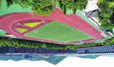
VI. F IELD E XPERIMENTS In this paper, we solve the problem of 3D placement of
As shown in Figure 15, our testbed consists of 7 DJI UAVs to achieve directional coverage. The key novelty of this
Phantom 4 advanced UAVs and 15 randomly distributed face paper is on proposing the first algorithm for UAV placement
figures as objects, and our experimental site is the playground with optimized directional coverage utility in 3D environment.
of our school including its stands, whose size is 110 m×80 m. The key contribution of this paper is building the practical
Specifically, we set α = 35◦ , β = 20◦ , D = 10 m, γmin = 3D directional coverage model, developing an approximation
10◦ , γmax = 70◦ , and θ = π/6 based on real hardware algorithm, and conducting simulation and field experiments for[4] L. Gupta et al., “Survey of important issues in UAV communication
networks,” IEEE Communications Surveys & Tutorials, 2016.
[5] “https://www.dji.com/phantom-4-adv/info.”
[6] V. Blanz et al., “Face recognition based on frontal views generated from
non-frontal images,” in IEEE CVPR, 2005.
[7] Y. C. Wang et al., “Using Rotatable and Directional (R & D) Sensors
to Achieve Temporal Coverage of Objects and Its Surveillance Appli-
cation,” IEEE TMC, 2012.
[8] Z. Wang and pthers, “Achieving k-barrier coverage in hybrid directional
sensor networks,” IEEE TMC, 2014.
[9] Y. Wang et al., “On full-view coverage in camera sensor networks,” in
IEEE INFOCOM, 2011.
[10] L. Li et al., “Radiation constrained fair charging for wireless power
transfer,” in ACM TOSN, 2018.
[11] H. Dai et al., “Wireless charger placement for directional charging,” in
IEEE TON, 2018.
[12] X. Wang et al., “Robust scheduling for wireless charger networks,” in
IEEE INFOCOM, 2019.
[13] ——, “Heterogeneous wireless charger placement with obstacles,” in
IEEE ICPP, 2018.
[14] N. Yu et al., “Placement of connected wireless chargers,” in IEEE
INFOCOM, 2018.
[15] H. Dai et al., “Optimizing wireless charger placement for directional
charging,” in IEEE INFOCOM, 2017.
[16] Z. Qin et al., “Fair-energy trajectory plan for reconnaissance mission
based on uavs cooperation,” in IEEE WCSP, 2018.
[17] K. Xie, L. Wang, X. Wang, G. Xie, and J. Wen, “Low cost and
high accuracy data gathering in wsns with matrix completion,” IEEE
Transactions on Mobile Computing, vol. 17, no. 7, pp. 1595–1608, 2018.
[18] K. Xie, X. Ning, X. Wang, S. He, Z. Ning, X. Liu, J. Wen, and Z. Qin,
“An efficient privacy-preserving compressive data gathering scheme in
wsns,” Information Sciences, vol. 390, pp. 82–94, 2017.
[19] K. Xie, X. Li, X. Wang, G. Xie, D. Xie, W. J. Li, Zhenyu, and Z. Diao,
(a) PANDA (b) GCDCS (c) GCOD “Quick and accurate false data detection in mobile crowd sensing,” in
IEEE INFOCOM 2019-IEEE Conference on Computer Communications,
Fig. 17: Experimental results of different algorithms 2019.
evaluation. The key technical depth of this paper is in reducing [20] H. Ma et al., “A coverage-enhancing method for 3d directional sensor
networks,” in IEEE INFOCOM, 2009.
the infinite solution space of this optimization problem to [21] L. Yupeng et al., “A virtual potential field based coverage-enhancing
a limited one by utilizing the techniques of space partition algorithm for 3d directional sensor networks,” in ISSDM, 2012.
and Dominating Coverage Set extraction, and modeling the [22] J. Peng et al., “A coverage-enhance scheduling algorithm for 3d direc-
tional sensor networks,” in CCDC, 2013.
reformulated problem as maximizing a monotone submodular [23] H.-J. Hsu et al., “Face recognition on drones: Issues and limitations,”
function subject to a matroid constraint. Our evaluation results in ACM DroNet, 2015.
show that our algorithm outperforms the other comparison [24] “https://enterprise.dji.com.”
[25] G. Fusco et al., “Selection and orientation of directional sensors for
algorithms by at least 75.4%. coverage maximization,” in IEEE SECON, 2009.
[26] T. Y. Lin et al., “Enhanced deployment algorithms for heterogeneous
ACKNOWLEDGMENT directional mobile sensors in a bounded monitoring area,” IEEE TMC,
This work was supported in part by the National Key R&D 2017.
[27] Z. Yu et al., “Local face-view barrier coverage in camera sensor
Program of China under Grant No. 2018YFB1004704, in networks,” in IEEE INFOCOM, 2015.
part by the National Natural Science Foundation of China [28] Y. Hu et al., “Critical sensing range for mobile heterogeneous camera
under Grant No. 61502229, 61872178, 61832005, 61672276, sensor networks,” in IEEE INFOCOM, 2014.
[29] X. Yang and other, “3D visual correlation model for wireless visual
61872173, 61472445, 61631020, 61702525, 61702545, and sensor networks,” in IEEE ICIS, 2017.
61321491, in part by the Natural Science Foundation of [30] C. Han et al., “An Energy Efficiency Node Scheduling Model for
Jiangsu Province under Grant No. BK20181251, in part by the Spatial-Temporal Coverage Optimization in 3D Directional Sensor Net-
works,” IEEE Access, 2016.
Fundamental Research Funds for the Central Universities un- [31] X. Yang and other, “3-D Application-Oriented Visual Correlation Model
der Grant 021014380079, in part by the Natural Science Foun- in Wireless Multimedia Sensor Networks,” IEEE Sensors Journal, 2017.
dation of Jiangsu Province under Grant No. BK20140076.5, [32] P. Si et al., “Barrier coverage for 3d camera sensor networks,” Sensors,
2017.
in part by the Nature Science Foundation of Jiangsu for [33] M. Hosseini et al., “Sensor selection and configuration in visual sensor
Distinguished Young Scientist under Grant BK20170039. networks,” in IST, 2012.
[34] J. Peng et al., “A coverage detection and re-deployment algorithm in 3d
R EFERENCES directional sensor networks,” in CCDC, 2015.
[1] S. He et al., “Full-view area coverage in camera sensor networks: [35] M. R. Gary et al., “Computers and intractability: A guide to the theory
Dimension reduction and near-optimal solutions,” IEEE TVT, 2016. of np-completeness,” 1979.
[2] X. Gao et al., “Optimization of full-view barrier coverage with rotatable [36] J. D.S, “Euler’s gem: The polyhedron formula and the birth of topology,”
camera sensors,” in IEEE ICDCS, 2017. Elsevier, vol. 6, 2008.
[3] S. Hayat et al., “Survey on unmanned aerial vehicle networks for [37] S. Fujishige, Submodular functions and optimization, 2005.
civil applications: A communications viewpoint,” IEEE Communications
Surveys & Tutorials, 2016.You can also read