Patience Is Power: Bargaining and Payoff Delay
←
→
Page content transcription
If your browser does not render page correctly, please read the page content below
Patience Is Power: Bargaining and Payoff Delay∗

                        Jeongbin Kim†                                Wooyoung Lim‡

                                  Sebastian Schweighofer-Kodritsch§

                                              March 12, 2021

                                                   Abstract
          We provide causal evidence that patience is a significant source of bargaining power. To
      do so, we first generalize the Rubinstein (1982) bargaining model to any positive discounting,
      maintaining only the assumption that preferences are dynamically consistent across bargaining
      rounds, and characterize the unique equilibrium. We then experimentally implement a version of
      this game, where bargaining delay is negligible (frequent offers), so that dynamic consistency holds
      by design, while bargainers nonetheless face significant payoff delay upon disagreement, and we
      induce different time preferences by randomly assigning individuals their own payoff delay profile
      (week or month per round, with or without front-end delay). Our leading treatment tests the
      prediction of a general patience advantage, independent of any details of discounting, which we
      strongly confirm. Additional treatments show that this advantage hinges on the presence of
      immediate payoffs and reject exponential discounting in favor of present-biased discounting.
      Keywords: Alternating-Offers Bargaining, Time Preferences, Present Bias, Laboratory Experiments
      JEL Classification: C78, C91, D03

  ∗
     We are grateful to Andreas Blume, Anujit Chakraborty, Dongkyu Chang, Pedro Dal Bó, Michael Böhm, John
Duffy, Yoram Halevy, Christina Gravert, Emin Karagözoğlu, Shih En Lu, Johannes Maier, Philip Neary, Thomas
Palfrey, Ariel Rubinstein, Klaus Schmidt, Peter Norman Sørensen, Charles Sprenger and Egor Starkov for valuable
comments and suggestions. For helpful comments and discussions, we thank seminar participants at Caltech, HKUST,
Hong Kong Baptist University, KAIST, National Taiwan University, Peking University Guanghua School, University
of Bonn (briq), University of Copenhagen, University of Hong Kong, University of Vienna, and conference/workshop
participants at the 2018 HKUST Workshop on Experimental Economics, the 2019 SUFE Workshop of Behavioral and
Experimental Economics, the 2019 CPMD Workshop on Behavioural and Experimental Economics at University of
Technology Sydney, the 2019 ESA World Meeting at Simon Fraser University, and the 2020 CESifo Area Conference on
Behavioral Economics (virtual). This study is supported by a grant from the Research Grants Council of Hong Kong
(Grant No. GRF-16500318), and Sebastian Schweighofer-Kodritsch also gratefully acknowledges financial support from
the Deutsche Forschungsgemeinschaft (through CRC TRR 190). The paper was previously circulated and presented
under the title “Bargaining and Time Preferences: An Experimental Study”.
   †
     National University of Singapore, Business School, 15 Kent Ridge Dr., Singapore 119245.                Email:
bizkj@nus.edu.sg. Phone: (65) 6516-4522. Fax: (65) 6779-5941.
   ‡
     The Hong Kong University of Science and Technology, Department of Economics, Kowloon, Hong Kong. Email:
wooyoung@ust.hk. Phone: (852) 2358-7628. Fax: (852) 2358-2084.
   §
     Humboldt-Universität zu Berlin, School of Business and Economics, Spandauer Str. 1, 10178 Berlin. Email:
sebastian.kodritsch@hu-berlin.de. Phone: (49) 30-2093-99497. Fax: (49) 30-2093-99491.
1 Introduction
How will two parties to a transaction divide the economic surplus that it creates? This distributional
question is a classic economic problem known as the bargaining problem, and it arises in numerous
settings.1 To theoretically resolve this problem with a clear prediction boils down to developing a
theory of bargaining power.
The seminal work of Rubinstein (1982) that initiated modern non-cooperative bargaining theory
achieves this by explicitly modeling bargaining as a dynamic game, in which disagreement leads to
costly delay of payoffs, and it identifies patience as a general source of an individual’s bargaining power.
Greater patience means greater willingness to delay agreement for a better deal, and in recognition
of this, the opponent is led to offer (or agree to) a better deal right away. The benefit to greater
patience extends to incomplete information about time preferences in the sense that it is beneficial
to be perceived as more patient (Rubinstein, 1985).2 In looser terms, the basic claim that being
more patient or being perceived as more patient confers an advantage in bargaining also appears in
consultants’ guides to negotiation,3 and it adds a strategic perspective on the positive correlation
between individuals’ patience and their long-run economic success (see, e.g., Mischel, Shoda, and
Rodriguez, 1989; Sunde, Dohmen, Enke, Falk, Huffman, and Meyerheim, 2020).4
Yet, to the best of our knowledge, there exists no direct evidence to substantiate this prediction
or claim. In fact, the only controlled bargaining study in which disagreement actually results in time
delay of payoffs concludes that time preferences do not matter in bargaining, in stark contradiction to
theory (Manzini, 2001).
In this paper, we offer not only direct but causal evidence on the effect of time preferences (in par-
ticular, patience) on bargaining. We achieve this by experimentally inducing different time preferences
between otherwise essentially identical groups of participants whom we match to bargain. Following
this causal approach, we obtain two main results. First, we find that patience is indeed a significant
source of bargaining power. Thus, we empirically substantiate the aforementioned general prediction
and claim. Second, we find that also in this strategic context the notion of patience has to be qualified
to distinguish between the immediate short run and the longer run: Based on what observed bargain-
ing behavior in our experiment reveals, exponential discounting is rejected in favor of present-biased
time discounting. This constitutes first evidence that people strategically respond to and exploit the
1
For instance, it arises within households (e.g., Browning and Chiappori, 1998), between workers and firms (e.g.,
Hall and Milgrom, 2008), as well as between firms (e.g., Ho and Lee, 2017) or between nations (see Powell, 2002, for a
survey of bargaining theory in political science analyses of international conflict).
2
See also Chatterjee and Samuelson (1987) and Bikhchandani (1992). The strategic advantage of greater patience
similarly prevails under reputational incentives (e.g., Abreu and Gul, 2000; Compte and Jehiel, 2002).
3
For instance, as in “Be patient—and show it” (Korda, 2011, p. 107) or “Patience is a key characteristic of the good
negotiator” (Forsyth, 2009, p. 160).
4
The importance of bargaining for individuals’ long-run economic outcomes has received particular attention in the
literature relating gender inequality and wage bargaining (e.g., Bowles, Babcock, and Lai, 2007; Sin, Stillman, and
Fabling, 2020). See Babcock and Laschever (2003, p. 5) for a drastic numerical example illustrating how important even
a single wage bargain can potentially be in generating inequality.
2present bias in others.
To structure our study, we adopt Rubinstein’s classic bilateral alternating offers protocol without
a deadline.5 Our key innovation is to disentangle bargaining delay (i.e., the time delay in bargaining
due to disagreement in a round) from payoff delay (i.e., the time delay of payoffs due to disagreement
in a round), which allows us to induce different time preferences among bargainers. Specifically, we
let all bargaining take place in a single session, so that bargaining delay is negligible (frequent offers),
while at the same time imposing significant payoff delay, of either a week or a month per round of
disagreement. Importantly, we exogenously and transparently vary this payoff delay at the individual
level (including also whether someone additionally faces a front-end delay): These payoff delay types
are randomly assigned and made common knowledge within every bargaining match (so we do not
induce incomplete information). Thus, we create groups of bargainers that are essentially identical
in every respect other than their effective time preferences, and we can compare bargaining behavior
and outcomes between different matches to identify causal effects due to people’s underlying time
preferences.
From a theoretical point of view, this method, which we call the effective discounting procedure,
permits clean comparative statics tests in time preferences.6 Our choice of specific treatments (corre-
sponding to pairings of types) is guided by two objectives: First, we aim to obtain and test general
predictions that essentially rely only on positive time discounting, to establish whether greater patience
is indeed a strategic advantage; second, we aim to additionally obtain and test discounting-specific
predictions that allow us to discriminate between different classes of time preferences based on what
bargaining behavior indirectly reveals about our participants’ underlying time preferences.
We show that under the assumption of exponential discounting (EXD), the games we implement
reduce to versions of those analyzed in Rubinstein (1982). The reason is that EXD implies dynamic
consistency, so only payoff delay matters, not bargaining delay. (Note that front-end delay is irrelevant,
akin to a fixed cost, and we implement constant payoff delay per round.) However, we would not want
to reject the notion that patience is power in bargaining based solely on a failure of EXD, which is
anyways well documented in time preferences research (e.g., Frederick, Loewenstein, and O’Donoghue,
2002; Augenblick, Niederle, and Sprenger, 2015; O’Donoghue and Rabin, 2015). Hence, we theoretically
extend the model of Rubinstein (1982) to general discounted utility, prove existence and uniqueness of
(perfect) equilibrium, which always has immediate agreement, and characterize it in terms of the two
parties’ time preferences. This result provides the basis for the comparative statics predictions in our
5
To ensure the credibility of our experiment and limit potential effects due to incomplete information, we additionally
impose a commonly known and constant 25% chance of random termination after any disagreement. Strictly speaking,
when we refer to time preferences, these should therefore be taken to include this risk; arguably, however, time preferences
inherently include attitudes to uncertainty (see Chakraborty, Halevy, and Saito, 2020).
6
We would like to thank John Duffy for helping us coin this term. A version of the method varying discounting
between but not within matches was introduced by one of us in Kim (2020b) to study the effect of time preferences
on cooperation in an indefinitely repeated prisoners’ dilemma, which theoretically exhibits equilibrium multiplicity,
however. As there, we use the convenient mobile app Venmo for all payments, including immediate payments.
3experiment, for various deviations from EXD, in particular the most commonly considered alternative
of quasi-hyperbolic (β, δ)-discounting (QHD, see Phelps and Pollak, 1968; Laibson, 1997). The only
substantial assumption we impose here is that of dynamic consistency of preferences across rounds of
bargaining. While generally a strong assumption, of course, it is satisfied in our experiment by design:
Negligible bargaining delay implies that only a single dated self of any individual gets to make all
decisions.7 A forteriori, also any naı̈veté (in the sense of O’Donoghue and Rabin, 1999) or mutual
learning about naı̈veté are irrelevant here.
The leading treatment WM achieves our first objective of testing for a patience advantage inde-
pendent of details of underlying time preferences. It matches bargainers whose payoff is delayed by
one week per round of disagreement (“weekly bargainers”) with bargainers for whom this is one month
(“monthly bargainers”), and we observe both versions of the game, differing in the type of the initial
proposer. Weekly bargainers are generally predicted to be at an advantage over monthly bargainers,
holding constant their initial role, and we strongly confirm this prediction.8 Hence, patience is indeed
a significant source of bargaining power.
The remaining two treatments WM2D and WW1D further allow us to determine the robustness
of this result and discriminate between discounting models based on a revealed preference argument.
Treatment WM2D is similar to WM, except that every bargainer’s payoff comes with an additional
front-end delay of one week (hence, this delay applies to immediate agreements, and we call these
bargainers “delayed”). While we still observe an advantage of weekly over monthly bargainers, it
is much smaller than in WM, showing that the patience advantage is mainly about differences in
short-run patience.
Treatment WW1D matches a weekly and a delayed weekly bargainer. Under EXD, the front-end
delay is irrelevant, and outcomes should be the same, irrespective of which type gets to make the initial
proposal. However, if discounting exhibits a present bias (such as under QHD), we should observe that
delayed weekly bargainers enjoy a significant advantage over non-delayed weekly bargainers. This is
indeed what we find, and it shows in particular that participants perceive and strategically respond
to a present bias in others.
In addition to these main results, our treatments permit comparisons between treatments, fixing
a given payoff type against two different opponent types (weekly bargainers in Treatments WM vs.
WW1D and delayed weekly bargainers in Treatments WM2D vs. WW1D). Analyzing these, on the
one hand, we are able to establish robustness of our leading result, confirming a generally predicted
patience advantage; on the other hand, we also find at least suggestive evidence that, beyond present
7
In this regard, our design is similar to the standard time preference elicitation paradigm where participants’ choose
between variously delayed monetary rewards at a single point in time. Relatedly, our design faces no selection issues,
whereas with significant bargaining delay, attrition is likely to be systematically related to time preferences (see Sprenger,
2015); e.g., Kim (2020a) indeed finds that patience and present bias measured at the beginning of his experiment closely
predicted how long participants would take part in his longitudinal study.
8
To test for this advantage, we compare distributions of initial proposals for first-order stochastic dominance; impor-
tantly, we obtain similar results when comparing accepted initial proposals.
4bias, bargainers perceive and respond to diminishing impatience, as in general hyperbolic discounting
(Loewenstein and Prelec, 1992).
Since our design does not itself induce incomplete information, we derive and test comparative
statics predictions from a complete information theory.9 In doing so, we essentially assume that the
behavioral effects due to any “natural” incomplete information are not systematically different between
the groups of matches we compare (analogous to “noise” in behavior). To address this issue, we consider
the rate(s) of immediate agreement: This rate is overall high, close to 75%, and, importantly, it is
similar across all kinds of matches/games we observe. This is evidence that incomplete information
is non-negligible, but that our design was successful in keeping its effects both relatively mild and
roughly constant (see related footnote 5).
Nonetheless, from this more general perspective, our experimental manipulation may be mainly one
of beliefs about patience. To investigate this question, we also measured time preferences using standard
methods for a subsample of our participants (after bargaining). We indeed find no robust correlations
between bargaining behavior and these measures at the individual level. This highlights the critical
importance of beliefs in strategic interaction and of controlling them experimentally. Regarding the
substantial interpretation of our main results this adds only a minor twist, however, because if beliefs
about patience matter strategically, then (knowledge of) patience does so.
Overall, we conclude that time preferences are certainly not all that matters in bargaining, but
they do matter significantly. Moreover, they do so in a manner that is theoretically predicted by and
consistent with what we know from the large body of work that has researched them, in particular
a present bias and diminishing impatience. Though the notion of patience is therefore more complex
than under EXD, it is generally a significant source of bargaining power.
The rest of this paper is organized as follows. We first present the general theoretical background
for our experimental study in Section 2. This is followed by a description of our experimental design,
including the behavioral predictions for the most important classes of time preferences, in Section 3.
We then report and discuss the findings from our experiment in Section 4, and subsequently relate
our study to the existing literature in Section 5. Section 6 offers concluding remarks. All proofs
are relegated to this paper’s Appendix. An Online Appendix consists of five parts and provides the
following supplemental material: additional figures that complement those in the main body of the
paper (part A); the results of alternative statistical tests (part B); experimental instructions and
selected screenshots for one exemplary experimental treatment (Treatment WM, parts C and D); all
details of our additional time preference elicitation and results on how measured time preferences relate
to bargaining behavior (part E).
9
Explicitly modeling incomplete information about time preferences to capture the observed heterogeneity seems
elusive. Fanning and Kloosterman (2020) successfully apply this alternative approach to study fairness concerns.
52 Theoretical Background
We now present the bargaining game that we implement in our experiment, characterize its unique
equilibrium under full generality with regard to time preferences, and show how it is a generalization
of the classic Rubinstein (1982) model. In doing so, we highlight two alternative interpretations of
the latter in terms of the timing of offers versus payoffs and point out how each of these relates to
assumptions about time preferences. All formal proofs are in the Appendix.
2.1 The Model
Consider two individuals i ∈ {1, 2} deciding on how to share a fixed monetary amount via indefinite
alternating-offers bargaining as in Rubinstein (1982). For simplicity, normalize the amount to one, so
divisions correspond to shares, and assume it is perfectly divisible. In any round n ∈ N, one individual
i proposes a division x ∈ {(x1 , x2 ) ∶ x1 ∈ [0, 1] and x2 = 1 − x1 } to the other individual j = 3 − i (we will
use this convention for i and j throughout), who can then either accept or reject. If the proposal is
accepted, there is agreement, and the game ends; if the proposal is rejected, then the game continues
to round n + 1, where this protocol is repeated with reversed roles such that j proposes and i responds.
Player 1 makes the proposal in round 1, and the game continues until a proposal is accepted. Denoting
by rn the responding player of round n, rn = 2 for n odd, and rn = 1 for n even.
We define an individual i’s preferences over the domain of her agreement outcomes (q, n) ∈
([0, 1] × N) ∪ {(0, ∞)}, where q denotes i’s share under the agreement and n denotes the round in
which it is reached, and where (0, ∞) subsumes any infinite history (perpetual disagreement). We
assume that i’s preferences at any point in the game are represented by a single utility function
Ui (q, n) = di (n − 1) ⋅ ui (q) ,
consisting of a delay discounting function di and an atemporal utility function ui such that
1. (Delay Discounting) di (0) = 1 > di (n) > di (n + 1) > 0 = di (∞) for all n ∈ N;
2. (Atemporal Utility) ui ∶ [0, 1] → [0, 1] is continuous and strictly increasing from u (0) = 0 to
u (1) = 1;10
3. (Intertemporal Utility) There exists αi < 1 such that for all n ∈ N, and for all q ∈ [0, 1) and
q ′ ∈ (q, 1],
i (δi (n) ⋅ ui (q )) − ui (δi (n) ⋅ ui (q)) ≤ αi ⋅ (q − q) ,
u−1 ′ −1 ′
where δi (n) ≡ di (n) /di (n − 1).
10
The assumption that u (1) = 1 is a mere normalization and without loss of generality.
6The discounting function di (n − 1) gives the discount factor for the total payoff delay associated
with agreement being reached in round n, i.e., after (n − 1) rounds of disagreement. The expression
δi (n) is the discount factor for the specific period of payoff delay caused by disagreement in round n;
by property 1, it lies between zero and one. Note that di (n) = ∏nm=1 δi (m) holds true.
Properties 1 and 2 define the bargaining problem: On the one hand, any round of disagreement
causes (further) payoff delay, which is costly to both individuals because they are impatient, and on
the other hand, each of them always wants more of the cake for herself.
Property 3 will guarantee uniqueness of equilibrium by ensuring that backwards-induction dy-
namics are well-behaved. It says that i’s willingness to pay to avoid another round’s payoff delay is
always increasing in the amount that she would obtain in case of this delay. This property extends
what has been termed “increasing loss to delay” (see the axiomatic formulation of Rubinstein, 1982
and its treatment in Osborne and Rubinstein, 1990) or “immediacy” (see the utility formulation of
Schweighofer-Kodritsch, 2018) to the non-stationary setting studied here, and it is implied by standard
assumptions; e.g., ui concave and supn δi (n) < 1.11
2.2 Equilibrium
Our equilibrium notion for this extensive-form game of perfect information is that of subgame perfect
Nash equilibrium (SPNE). SPNE outcomes of a more general version of this game, where bargaining
is over a general time-varying surplus, are geometrically analyzed by Binmore (1987), who shows that
the extreme utilities are obtained in history-independent SPNE. Coles and Muthoo (2003) establish
existence for a version that also contains our model. We contribute here a uniqueness result and
a characterization for general discounted utility where non-stationary discounting is the source of
time-varying surplus, and we provide algebraic proofs.
Lemma 1. There exists a unique sequence xn such that, for all n ∈ N,
xn = 1 − u−1
rn (δrn (n) ⋅ urn (xn+1 )) . (2.1)
Proposition 1. There exists a unique equilibrium. This unique equilibrium is in history-independent
strategies that imply immediate agreement in every round. It is characterized by the unique sequence
xn of lemma 1 as follows: in round n, the respective proposer demands share xn , and the respective
respondent accepts a demand q if and only if q ≤ xn .
11
Let u be concave, q0 < q1 and ε > 0. Then
u (q0 + ε) − u (q0 ) u (q1 + ε) − u (q1 ) δu (q1 + ε) − δu (q1 )
≥ >
ε ε ε
for any δ < 1. Moreover, if u (q0 ) = δu (q1 ), then u (q0 + ε) > δu (q1 + ε) follows immediately from the above. This is
equivalent to ε > u−1 (δu (q1 + ε)) − q0 and upon substituting q0 = u−1 (δu (q1 )) to ε > u−1 (δu (q1 + ε)) − u−1 (δu (q1 )).
Denoting q ≡ q1 and q ′ ≡ q1 + ε, and applying this to individual i’s preferences, the third assumed property follows for
any given n; supn δi (n) < 1 ensures boundedness away from equality across all n by ruling out that limn→∞ δ (n) → 1.
7Proposition 1 delivers a general characterization of SPNE. It has the familiar property that in
each round, the proposer makes the smallest acceptable offer to the respondent, given the unique
continuation agreement that results upon rejection. Hence, in terms of time preferences as of a given
round n, only the respondent’s discount factor for that round’s delay δrn (n) enters the equilibrium
outcome. In the special case where the model reduces to the benchmark of Rubinstein (1982), the
infinite sequence in (2.1) reduces to two equations:
x1 = 1 − u−1
2 (δ2 ⋅ u2 (x2 )) ,
x2 = 1 − u−1
1 (δ1 ⋅ u1 (x1 )) .
We generate several behavioral predictions from this exponential-discounting benchmark for our con-
crete experimental treatments, and we employ the general characterization to also derive the behavioral
predictions under various alternative forms of discounting (in particular, quasi-hyperbolic discounting
capturing a present bias). We present all of these theoretical predictions in Section 3 after defining
our specific treatments.
2.3 Remarks
The only substantial assumption we impose on preferences is dynamic consistency across rounds of
bargaining, i.e., that there is a single utility function representing an individual’s preferences at any
point in the game. This implies that only the payoff delay due to disagreement matters, the bargaining
delay (i.e., the time delay until the next round) is irrelevant.12 Given this, our abstract formulation
of preferences in terms of rounds of agreement allows us to capture a huge variety of protocols and
preferences. For instance, even assuming symmetric exponential discounting, if the payoff delay due
to the first round of bargaining is longer than that due to any later round where it is constant, then
preferences take the quasi-hyperbolic form of di (n − 1) = βδ n−1 (n > 1), even though time preferences
are dynamically consistent. Under this assumption, we therefore essentially cover any combination
of time preferences and payoff (as well as bargaining) timings, and we establish a very general result
regarding equilibrium uniqueness and structure.13
In view of the vast body of evidence on time preferences, dynamic consistency of actual time pref-
erences would be a very strong assumption.14 What we impose, however, is only dynamic consistency
12
Formalizing bargaining and payoff delay requires explicitly accounting for time. Suppose round n takes place at
date τn and agreement in round n results in payoffs at date tn , where both τn and tn are increasing sequences, such
that τn ≤ tn holds (bargaining is never about past payoffs). The bargaining and the payoff delay due to disagreement in
round n are, respectively, the delay from date τn to date τn+1 and the delay from date tn to date tn+1 . The statement
that bargaining delay is irrelevant formally says that, for given tn , any τn such that τn ≤ tn yields the same game.
13
We focus on the separable case of discounted utility merely to notationally ease the exposition. It is relatively
straightforward to formulate the three assumed properties for non-separable preferences and to then generalize our
uniqueness and characterization result using the same line of proof.
14
See, however, Halevy (2015) for evidence that some violations of exponential discounting may be due to time variance
rather than dynamic inconsistency of discounting.
8of preferences across bargaining rounds, which is satisfied in the limiting case of frequent offers where
bargaining delay is negligible.15 Then, a single dated self of any individual makes all the strategic
decisions and only this one temporal snapshot of preferences matters (sometimes called “commitment
preferences”); thus, we are able to study general time preferences, including dynamically inconsis-
tent ones, without actually confronting any issues of dynamic inconsistency in the bargaining itself
(importantly including naı̈veté, see O’Donoghue and Rabin, 1999).
This is the bargaining version we implement in our experiment. It further offers the practical
advantage over the usual interpretation of alternating-offers bargaining, according to which bargaining
and payoff delay coincide, that there are no selection issues related to time preferences, neither into the
experiment nor during the running of the experiment. Moreover, if preferences really are dynamically
consistent (or individuals share a common belief in such consistency), it is equivalent to a game with
this usual interpretation: Proposition 1 and any behavioral predictions derived from it then directly
extend to the setting where bargaining itself takes time. This applies in particular to the special case of
our model with exponential discounting and constant payoff delay, which is that of Rubinstein (1982)
and will serve as our benchmark.
3 Experimental Design and Behavioral Predictions
3.1 Experimental Design
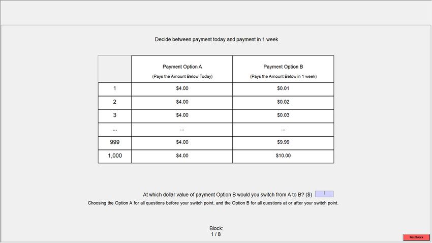
In line with the theory just developed, our experiment implements indefinitely alternating offers bar-
gaining games with frequent offers and significant payoff delay. The monetary surplus to be divided
is fixed and amounts to US$50. Table 1 presents our experimental design, which consists of three
treatments. Each of these treatments corresponds to a particular pairing of “bargainer types.” This
type is the exogenously imposed payoff delay profile that an individual faces, according to the effective
discounting procedure.
Table 1: Experimental Treatments
Bargainer 2
Bargainer 1
Monthly with D Monthly Weekly with D
Weekly with D WM2D N/A N/A
Weekly N/A WM WW1D
*Note: Delay (D) = 1 Week
In Treatment WM, one bargainer faces one week of delay per round of disagreement, whereas the
15
As long as payoff delay remains significant, the model is not susceptible to the “smallest-units” critique of van
Damme, Selten, and Winter (1990).
9other faces one month of such delay. Treatment WM2D is similar, but both bargainers additionally
face a front-end delay of one week so that immediate agreements are about payoffs to be received in one
week’s time. In Treatment WW1D, both bargainers face identical delays per round of disagreement of
one week, but one of them additionally faces a front-end delay of one week.
Every treatment therefore matches different payoff types. The treatment is public, whereby the
payoff delay types of any two matched participants are common knowledge. Moreover, who is assigned
to be the initial proposer is randomized at the match level, so we observe both kinds of games of any
treatment.
Weeks and months are both natural and significant time units, so our treatments should be able
to create meaningful differences in effective discounting. To credibly implement delayed payments, we
relied on the popular mobile payment system Venmo.16 In the rest of the paper, we will call a bargainer
type whose payment window is weekly/monthly/delayed a weekly/monthly/delayed bargainer.
For a concrete illustration of the different payoff delays, consider agreements that are reached in
Round 3. In Treatment WM, this would mean that the weekly bargainer receives the associated payoff
in two weeks from the day of the experiment, and the monthly bargainer in two months; in Treatment
WM2D, these delays would be three weeks for the delayed weekly and a week plus two months for the
delayed monthly bargainer; in Treatment WW1D, this would be two weeks for the weekly and three
weeks for the delayed weekly bargainer. Appendices C and D provide the instructions and selected
screenshots for exemplary Treatment WM.
While we could have tested for a patience advantage also with a finite-horizon version of the model,
there are two advantages to using the indefinite version. First, we can interpret our experiment as
the first test of the original Rubinstein (1982) model, which has no deadline and in which preferences
are defined over delayed payoffs (see Section 5 for related experimental work). Second, the absence
of a definite deadline should level the playing field with regard to participants’ ability to engage in
backwards induction.
We coupled this with a fixed, commonly known termination probability of 25% that was trans-
parently applied to all rounds of all games in all treatments (so it could not cause any systematic
differences). This serves three related purposes. First, it ensures that every bargaining game, while
indefinite, is still expected to end after a reasonable amount of time, which is important for the credi-
bility and smooth running of our experiment. Second, it limits the potential importance of incomplete
information by making screening and signaling additionally costly. Third, it theoretically keeps bar-
gainers further away from possible indifference to delay, as required by Property 3 of our preference
16
Venmo is a service provided by PayPal that allows account holders to transfer funds to others via a mobile phone
app. It handled $12 billion in transactions during the first quarter of 2018 (https://en.wikipedia.org/wiki/venmo). For
more information, please visit https://help.venmo.com/hc/en-us/articles/210413477. When recruiting our participants,
we clearly announced that those without a Venmo account were not eligible to participate in the experiment. At the end
of the experiment, the participants were asked to report their account information for payment, including username and
email address details. None of the participants reported any error or difficulty in providing this information, suggesting
that all our participants were sufficiently familiar with Venmo in their daily lives.
10assumptions. Of course, in terms of the model, discounting should therefore be interpreted as also
including this constant risk (assuming expected utility).17
3.2 Behavioral Predictions
We now employ Proposition 1 to derive the comparative statics predictions related to time preferences
that our experiment is designed to test. We begin by establishing the important and influential bench-
mark predictions from exponential discounting, as in Rubinstein (1982), then we derive the differential
predictions under its leading alternative, quasi-hyperbolic discounting, and finally we discuss predic-
tions under various other forms of discounting as they appear in the literature on time preferences.
This will show that the leading treatment WM allows us to test for a general patience advantage,
and the remaining two treatments WM2D and WW1D allow us to investigate the robustness of this
hypothesized advantage as well as discriminate between different classes of time preferences based on
a revealed preference argument. All formal proofs are in the Appendix.
In each case, to capture the implied typical behavior, we impose preference symmetry: i.e., both
individuals have the same atemporal utility function, u1 = u2 = u, and for the same future delay ∆t,t′
from some given date in time t to some later date t′ > t, discount utility with the same discount
factor δt,t′ . Our effective discounting procedure induces different time preferences by implementing
idiosyncratic payoff delay profiles (types).
Recall that the only universal prediction from Proposition 1 is immediate agreement. We formulate
the comparative statics predictions in terms of relative bargaining power, as reflected in this immediate
agreement. For predictions within a treatment that matches two bargainer types A and B (e.g., weekly
and monthly bargainers in Treatment WM ), call the game where type A is the initial proposer AB-
game and the game where type B is the initial proposer BA-game; we then say that the type A
bargainer is stronger than the type B bargainer if the type A bargainer’s equilibrium share in
the AB-game is greater than the type B bargainer’s equilibrium share in the BA-game.18 If neither type
is stronger than the other in the above sense, we say they are equally strong. For between-treatment
predictions, additionally consider another treatment that matches types A and C; we then say that
the type A bargainer is stronger against the type B bargainer than against the type C
bargainer as initial proposer (resp., respondent) if type A bargainer’s equilibrium share in the
AB-game (resp., BA-game) is greater than type A bargainer’s equilibrium share in the AC-game (resp.,
17
With expected utility, a constant probability of breakdown simply proportionally reduces each δi (n) by this fraction.
It should be noted, however, that certain violations of expected utility would yield dynamic inconsistency even across
rounds. In particular, Halevy (2008) argues that the future is inherently uncertain and shows how empirically plausible
non-linear probability weighting of future consumption risk provides a foundation of present bias and diminishing
impatience. Since Schweighofer-Kodritsch (2018) finds that this form of dynamic inconsistency does not upset any of
the qualitative equilibrium predictions of the benchmark under dynamic consistency, we theoretically abstract from risk
as a potential source of dynamic inconsistency.
18
This compares A and B as the initial proposer only; however, since shares add up to one, A is stronger than B as
the initial proposer if and only if A is stronger than B as the initial respondent.
11CA-game). If this is true both as initial proposer and initial respondent we simply say that the type
A bargainer is stronger against the type B bargainer than against the type C bargainer.19
Exponential Discounting (EXD). Since any given bargainer type faces a constant payoff delay,
the stationarity property of EXD implies that any such delay is discounted with the same discount
factor, irrespective of any front-end delay. Let δ ∈ (0, 1) be the (common) discount factor for a weekly
delay, and let φδ be the (common) discount factor for a monthly delay, where 0 < φ < 1 due to
impatience.20 Using notation φi ∈ {φ, 1} with φi = 1 if and only if bargainer i is a weekly bargainer,
any bargainer i’s type is fully captured by φi , such that Ui (q, n) = (φi δ) u (q) and δi (n) = φi δ is
n−1
constant across rounds n. WM and WM2D both correspond to pairing {1, φ}, and WW1D corresponds
to pairing {1, 1}.
Prediction 1. Symmetric EXD implies:
(A1) In Treatment WM, the weekly bargainer is stronger than the monthly bargainer.
(A2) In Treatment WM2D, the weekly bargainer is stronger than the monthly bargainer.
(A3) In Treatment WW1D, the weekly bargainer and the delayed weekly bargainer are equally strong.
(B1) Between Treatments WM and WW1D, the weekly bargainer is stronger against the monthly
bargainer than against the delayed weekly bargainer.
(B2) Between Treatments WM2D and WW1D, the delayed weekly bargainer is stronger against the
delayed monthly bargainer than against the weekly bargainer.
These predictions are straightforward. Simply note that under EXD front-end delay is irrelevant,
and weekly bargainers have a higher effective discount factor than monthly bargainers, i.e., they are
effectively more patient.
Quasi-Hyperbolic Discounting (QHD). Present bias, the excessive weight put on immediate
rewards relative to delayed rewards, is the most important deviation from EXD. By adding a single
parameter β ∈ (0, 1), the model of quasi-hyperbolic discounting parsimoniously captures this empir-
ically well-established phenomenon. The bias may here play a role only in the first round because
upon failure to agree immediately, all possible payoffs lie in the future. Moreover, it will do so only
when the initial respondent faces no front-end delay because the proposer’s discounting of the first
round’s delay is irrelevant anyways due to the proposer’s strategic advantage, and a front-end delay
19
In comparisons between treatments, the observation in footnote 18 does not apply. The fact that shares add up
to one only means that A is stronger against B than against C as the initial proposer if and only if B’s share in the
AB-game is smaller than C’s share in the AC-game, but does not imply anything about A’s share in the BA-game versus
A’s share in the CA-game.
20
If we take a month to equal four weeks, then φδ = δ 4 pins down φ = δ 3 .
12for the respondent pushes any immediate-agreement payoff into the future. Keeping the earlier EXD
notation and adding βi ∈ {β, 1} with βi = 1 if and only if bargainer i is not delayed, any bargainer
i’s type is fully captured by (φi , βi ), such that Ui (q, n) = βi (φi δ) u (q); now δi (1) = βi φi δ and, for
n−1
n > 1, δi (n) = φi δ ≥ δi (1). WM corresponds to pairing {(1, β) , (φ, β)}, WM2D corresponds to pairing
{(1, 1) , (φ, 1)}, and WW1D corresponds to pairing {(1, β) , (1, 1)}. In the predictions under QHD
below we highlight those that differ from Prediction 1 under EXD.
Prediction 2. Symmetric QHD implies the same as symmetric EXD except:
(A3) In Treatment WW1D, the delayed weekly bargainer is stronger than the weekly bargainer.
(B2) Between Treatments WM2D and WW1D, the delayed weekly bargainer is stronger against the
delayed monthly bargainer than against the weekly bargainer as initial respondent, but there is
no general prediction concerning the weekly bargainer as initial proposer.
The predictions under QHD are straightforward from those under EXD, upon noting that (i)
Prediction 1 applies to the Round-2 subgame, where bargaining is only about delayed payoffs and QHD
coincides with EXD, and (ii) the immediate Round-1 agreement has the initial respondent indifferent
to the Round-2 agreement, so only the respondent’s discounting for the first round’s disagreement
matters. In particular, a present bias in the sense of β < 1 enters the actual equilibrium agreement
if and only if the initial respondent is not delayed, so ceteris paribus front-end delay makes an initial
respondent stronger.
Within Treatment WM, the weekly bargainer is therefore stronger than the monthly bargainer in
the Round-2 subgame, and since present bias applies equally to both types, this carries over to the
immediate Round-1 agreement. (Present bias here simply reinforces the proposer advantage.) The
QHD prediction within Treatment WM2D is immediate from that under EXD because present bias
is irrelevant. This is in stark contrast to Treatment WW1D, which is symmetric under EXD, but not
under QHD: Whereas the Round-2 subgame is symmetric, the delayed weekly bargainer is the stronger
initial respondent due to the effective absence of a present bias. (Equivalently, this type is stronger as
the initial proposer because it faces a weaker respondent.)
The observation that under QHD front-end delay is advantageous as initial respondent implies that
the EXD prediction between Treatments WM and WW1D is only reinforced under QHD regarding
the weekly bargainer as initial proposer, since the delayed weekly respondent then faces no present bias
whereas the monthly one does. For the weekly bargainer as the initial respondent, present bias equally
weakens this type irrespective of the type of proposer and does not affect the comparison relative to
EXD.
Between Treatments WM2D and WW1D, when the delayed weekly bargainer is the initial respon-
dent, the game under QHD is the same as that under EXD, so the prediction immediately carries
over. However, when the delayed weekly bargainer is the initial proposer, present bias is effective in
13WW1D but not in WM2D; while the Round-2 agreement is less favorable with a weekly opponent
than a delayed monthly one, the former is therefore weakened by present bias, whereas the latter is
not. This means that the comparison depends on how strong present bias is relative to the difference
in long-run discounting, so there is no general prediction under QHD.
Our focus here lies on comparative statics predictions specific to time preferences. These are
predicated on immediate agreement equilibrium. We investigate this universal prediction and discuss
the interpretation of our findings in the absence of immediate agreement in Section 4.3. There, we
also discuss another commonly considered comparative statics prediction due to the alternating-offers
protocol’s inherent asymmetry, which is that of a proposer advantage. This prediction is not specific to
payoff delay as the cost of disagreement, but it does obtain here as well (under both EXD and QHD). A
proposer advantage is a within-treatments prediction, and in the terminology introduced earlier, type
A has a proposer advantage if this very type’s equilibrium share is greater in the AB-game than in
the BA-game. Note that this is true if and only if type B has a proposer advantage. This comparison
concerns a given type in the two different initial roles, whereas the patience advantage compares the
two different types in the same initial role. It is easily verified that neither advantage implies nor rules
out the other.
Other Forms of Discounting. Due to the tractability they afford, EXD and QHD are, by far,
the most important models of time preferences for theoretical analyses. However, empirical studies,
especially from psychology, suggest hyperbolic discounting (HYD)—a form of diminishing impatience,
which implies present bias—as the “universal” form of discounting (for discussion see Frederick et al.,
2002). At the same time, experimental studies from economics also document the opposite of present
bias, namely (near-) future bias (see, e.g., Ebert and Prelec, 2007; Bleichrodt, Rohde, and Wakker,
2009; Takeuchi, 2011). We now discuss the implications of these alternatives.
First, consider diminishing impatience, meaning δi (n) increases in n. This implies a present bias,
so a front-end delay increases such a discounter’s bargaining power as the respondent. However,
disagreement in round n adds a shorter basic payoff delay to a shorter existing delay for a weekly
bargainer than for a monthly bargainer, meaning that for n large enough, even a monthly bargainer
may in general become more patient than a weekly bargainer. This could resonate through the entire
recursion of equation (2.1), thereby affecting the equilibrium outcome. Based on the intuition that
discounting for the same additional delay would not change too quickly with the preceding delay
(except for the immediate present) and in view of the sizable termination probability, we would assume
that the effect of pushing a basic delay further into the future does not outweigh that of the basic
delay being longer in determining the immediate equilibrium agreement. Indeed, the most general
model of HYD proposed by Loewenstein and Prelec (1992), which we will identify with HYD in what
follows, imposes the structure of d(t) = (1 − α ⋅ t)−β/α (with α, β > 0), and this implies that a weekly
bargainer always remains more patient than a monthly bargainer; notably, this extends also to when
14both are delayed.21 We therefore immediately obtain the same predictions within Treatments WM and
WM2D. Regarding Treatment WW1D, the delayed weekly bargainer is only further strengthened by
diminishing impatience, so the prediction under QHD extends to HYD. For a similar reason—since the
weekly bargainer is always more patient than the monthly bargainer, the delayed weekly bargainer is
so—the prediction between Treatments WM and WW1D, which is common to both EXD and QHD,
carries over with this model of HYD. However, it still depends on parameters whether the weekly
bargainer or the delayed monthly bargainer is always more patient (though one can show that one is).
This renders HYD altogether permissive with respect to the comparison between Treatments WM2D
and WW1D.
Finally, consider near-future bias. Somewhat loosely, this means that the discounting function is
initially concave (hump-shaped), in contrast to the convex discounting functions under EXD, QHD or
HYD. While empirically documented, it is neither known how prevalent this bias is (hence, whether
it could be reasonably expected to guide typical behavior) nor how far the near future extends from
the immediate present (hence, whether a week’s front-end delay would mute it). In view of these
open issues, we omit a detailed analysis but note that if a near-future bias operates like an “inverted”
present bias in the QHD model—i.e., 1 < β < 1/δ—then a front-end delay would make the initial
respondent weaker rather than stronger. Hence, in Treatment WW1D, the weekly bargainer rather
than the delayed weekly bargainer would be stronger. Using that βφ < 1, which follows from β < 1/δ
and φ < δ, it is straightforward to show that the between-treatment predictions under such near-future
bias coincide with those under EXD.
3.3 Administrative Details
Our experiment was conducted using z-Tree (Fischbacher, 2007) at the University of California, Irvine.
A total of 348 subjects who had no prior experience with our experiment were recruited from the
graduate and undergraduate student population of the university. Upon arrival at the laboratory,
the participants were instructed to sit at separate computer terminals. Each received a copy of the
experiment’s instructions. To ensure that the information contained in the instructions was induced
as public knowledge, these instructions were read aloud, and the reading was accompanied by slide
illustrations followed by a comprehension quiz.
Each session employed a single treatment, and we conducted 6 sessions for each treatment, for a
total of 18 sessions (6 sessions × 3 treatments). In all sessions, the participants anonymously played
10 games under the corresponding treatment condition, say matching bargainer types A and B, where
21
The reason is that the different delays per round have a constant ratio, which also equals the ratio of total delays
the two bargainers face in any agreement. Measuring time t in the unit that is the shorter delay per round and
letting the corresponding type be type A, A’s discount factor for round n is δA (n) = [(1 − α ⋅ n)/(1 − α ⋅ (n − 1))]−β/α ;
letting the longer delay be k > 1 times the shorter delay with corresponding type B, B’s discount factor for round n is
δB (n) = [(1 − α ⋅ kn)/(1 − α ⋅ k(n − 1))]−β/α . Basic algebra yields δA (n) > δB (n), and it is straightforward to check that
the same holds true if both A and B face the same front-end delay.
15bargaining was over how to divide 500 tokens worth $50. At the beginning of the experiment, one
half of the participants were randomly assigned to be Type A and the other half to be Type B.
Individual participants’ types remained fixed throughout the session. We used random rematching
across subsequent games, subject to the treatment condition of always matching a Type A and a Type
B. Any participant therefore always had the same type and always faced the same opponent type
to avoid any confusion regarding payoff delay profiles. However, the identity of the initial proposer
was always determined by chance, so we observe both kinds of games of any treatment, and every
participant would sometimes be the initial proposer and sometimes the initial respondent. Each
session had 16–20 participants and hence involved 8–10 simultaneous games.
At the end of the experiment, one of the 10 matches a participant had played was randomly selected
for payment.22 For the selected match, if agreement was reached, the agreed number of tokens for
this participant was converted into US dollars at a fixed and commonly known exchange rate of $0.1
per token, and the delay of the participant’s dollar payment was determined according to (1) his/her
bargainer type and (2) the round of the agreement.
After all ten bargaining matches were over, we additionally measured the participants’ time pref-
erences using a version of the BDM (Becker, DeGroot, and Marschak, 1964) method. We elicited
switching points (indifferences) between sooner and later money amounts. One decision was randomly
selected for actual payment.23
In addition, participants received a show-up payment of $10. Any amount a participant was due
to receive was paid electronically via Venmo, including immediate payments. Earnings were $37.90 on
average, and the average duration of a session was approximately 1.5 hours.24
4 Experimental Results
This section presents our experimental results regarding Predictions 1 and 2. We first consider the pre-
dictions within treatments, (A1)–(A3), and then those between treatments, (B1)–(B2). Subsequently,
we provide additional results and discussion concerning the robustness of our main analyses, immediate
vs. delayed agreement (relating to evidence for and effects of incomplete information), the potential
role of social preferences, and whether we observe a basic proposer advantage in our particular setting.
In line with the literature, we conduct our main tests based on observed initial proposals, as they
reveal the proposers’ perceptions of relative bargaining power. We have this data for every match.
22
Azrieli, Chambers, and Healy (2018) offer a theoretical justification and discussion of this payment rule’s incentive
compatibility in settings like ours.
23
We implemented the elicitation task in 4 sessions per treatment. This allows us to check whether the random
assignment was successfully implemented in terms of participants’ underlying time preferences, which is a crucial aspect
of our design and which our data confirm. See Appendix E for details.
24
We conducted 6 sessions in May and June 2018, and 12 sessions in October and December 2018. The longest delay
among the matches selected for payment was 7 months, and the corresponding amount was paid on May 17, 2019.
16Acknowledging potential preference heterogeneity and incomplete information, we take the pre-
dictions to concern shifts in the distribution of bargaining power between the different kinds of
games/matches that are compared. We therefore conduct our comparisons based on the entire ob-
served distributions of initial proposals (always in terms of the proposer’s claimed share). Specifically,
we always examine the cumulative distribution functions (CDFs) for first-order stochastic dominance
and use appropriate unidirectional Kolmogorov-Smirnov (KS) tests for statistical significance in this
strong sense;25 note that in contrast to comparisons of means, which are always ordered, such order is
not guaranteed here.
4.1 Within-Treatment Comparisons
Within treatments matching two types A and B, we compare initial proposals by type A to type B
(i.e., in the AB game) and initial proposals by type B to type A (i.e., in the BA game). When the
distribution of initial demands by type A in the AB game first-order stochastically dominates that of
initial demands by type B in the BA game, we say that type A bargainers are observed to be
stronger than type B bargainers. Since demands and offers add up to a constant amount (500
tokens), this is equivalent to type A’s facing an unambiguously more favorable distribution of initial
offers than type B.
(a) First 5 Matches (b) Last 5 Matches
Figure 1: Round-1 Proposals in Treatment WM
The most general prediction of a patience advantage concerns our leading treatment WM. Figure 1
presents the CDF of Round-1 proposals in this treatment aggregated over the first 5 matches (Figure
1(a)) and over the last 5 matches (Figure 1(b)) by bargainer type. The solid line indicates the CDF
25
The CDF figures that follow below are censored by the given range of [250, 310] for ease of graphical representation.
This range contains, on average, more than 95% of the observations in the data. Such truncation does not apply to any
of the statistical analyses.
17for the weekly proposer, and the dotted line indicates the CDF for the monthly proposer. Consistent
with prior findings, fairness concerns seem to be present.26 Approximately 50% of proposals are equal
(250-250) splits, though this varies strongly by type, with weekly bargainers much less likely to propose
an equal split than monthly bargainers. Indeed, regarding the key comparative statics prediction, the
CDF of proposals by weekly bargainers clearly lies below that for monthly bargainers already for the
first 5 matches (KS test, p-value = 0.046). This difference remains statistically significant and becomes
even more substantial in magnitude in the last 5 matches (KS test, p-value < 0.01).
Result 1 (Basic Delay Advantage in Treatment WM ). In Treatment WM, weekly bargainers are
observed to be stronger than monthly bargainers. This difference is statistically significant.
This result shows that weekly and monthly bargainers share a common perception about their
relative bargainer power, strongly favoring the former. Accordingly, we strongly confirm the basic
prediction (A1) that patience is a source of bargaining power.
(a) First 5 Matches (b) Last 5 Matches
Figure 2: Round-1 Proposals in Treatment WM2D
Treatment WM2D adds a front-end delay to both types and therefore allows us to investigate to
what extent this patience advantage is driven by short-run patience vs. long-run patience. Figure 2
presents the CDF of Round-1 proposals in this treatment by bargainer type. The solid line indicates
the CDF for the (now delayed) weekly proposer, and the dotted line indicates the CDF for the (now
delayed) monthly proposer. Again, close to 50% of proposals are equal splits, though here, these
are equally likely for both types. Unlike in Treatment WM, the distributions of proposals are quite
obviously not significantly different initially (KS test, p-value = 0.726). However, behavior gravitates
towards the theoretical prediction as the participants gain more experience. In the comparison for the
26
This does not require the proposers to be fair-minded themselves; it could be that they have “selfish” preferences
but believe they are facing a fair-minded respondent.
18You can also read