Negative interest rates, deposit funding and bank lending - Tan Schelling, Pascal Towbin
←
→
Page content transcription
If your browser does not render page correctly, please read the page content below
Negative interest rates, deposit funding
and bank lending
Tan Schelling, Pascal Towbin

SNB Working Papers
5/2020
Legal Issues

DISCLAIMER

The views expressed in this paper are those of the author(s) and
do not necessarily represent those of the Swiss National Bank.
Working Papers describe research in progress. Their aim is to
elicit comments and to further debate.

COPYRIGHT©

The Swiss National Bank (SNB) respects all third-party rights, in
particular rights relating to works protected by copyright (infor-
mation or data, wordings and depictions, to the extent that these
are of an individual character).

SNB publications containing a reference to a copyright (© Swiss
National Bank/SNB, Zurich/year, or similar) may, under copyright
law, only be used (reproduced, used via the internet, etc.) for
non-commercial purposes and provided that the source is menti-
oned. Their use for commercial purposes is only permitted with
the prior express consent of the SNB.

General information and data published without reference to a
copyright may be used without mentioning the source. To the
extent that the information and data clearly derive from outside
sources, the users of such information and data are obliged to
respect any existing copyrights and to obtain the right of use from
the relevant outside source themselves.

LIMITATION OF LIABILITY

The SNB accepts no responsibility for any information it provides.
Under no circumstances will it accept any liability for losses or
damage which may result from the use of such information.
This limitation of liability applies, in particular, to the topicality,
accuracy, validity and availability of the information.

ISSN 1660-7716 (printed version)
ISSN 1660-7724 (online version)

© 2020 by Swiss National Bank, Börsenstrasse 15,
P.O. Box, CH-8022 Zurich
Negative interest rates, deposit funding and bank
                            lending∗
                                 Tan Schelling† Pascal Towbin‡

                                            January 2020

                                               Abstract
            In a negative interest rate environment, banks have generally proved reluc-
        tant to pass on negative interest rates to their retail depositors. Thus, banks that
        are more dependent on deposit funding face higher funding costs relative to other
        banks. This raises questions about the effect of negative interest rates on bank
        lending and monetary policy transmission. To study the transmission of negative
        interest rates, we use an unexpected policy decision by the Swiss National Bank
        in combination with a comprehensive and granular micro data set on individual
        Swiss corporate loans. We find that banks relying more heavily on deposit fund-
        ing take more risks and offer looser lending terms than other banks. This result
        is consistent with the risk-taking channel, where a lower policy rate spurs bank
        risk-taking to maintain profits.

   ∗
      We thank Stefanie Behncke, Itzhak Ben-David, Toni Beutler, Robert Bichsel, Jürg Blum, Martin
Brown, Andreas Fuster, Christian Glocker, Tumer Kapan, Cathérine Koch, Cyril Monnet, Diane Pier-
ret, Oleg Reichmann, Olav Syrstad, Eric Zwick and participants at seminars at the SNB and IMF, the SNB
2018 research conference, SSES 2019 conference, and the CEPR-BCBS 2019 workshop for helpful com-
ments. The views, opinions, findings, and conclusions or recommendations expressed in this paper are
strictly those of the authors. They do not necessarily reflect the views of the Swiss National Bank (SNB).
The SNB takes no responsibility for any errors or omissions in, or for the correctness of, the information
contained in this paper.
    †
      Swiss National Bank, tan.schelling@snb.ch
    ‡
      Swiss National Bank, pascal.towbin@snb.ch

                                                    1
1 Introduction
Since 2012, several central banks have introduced negative interest rate policies for the
first time in history. While nominal market rates generally adjusted quickly, banks
have been reluctant to pass on negative interest rates to retail depositors. Conse-
quently, rates have been stuck at or near zero ever since. This zero lower bound on
deposit rates might be explained by the outside option of holding cash or by banks’
unwillingness to lower deposit rates out of fear of losing customers to competitors
(Eggertsson et al., 2019; Eisenschmidt and Smets, 2017; Heider et al., 2019). Given
the observed zero lower bound on deposit rates, we ask how deposit funding impacts
bank lending and monetary policy transmission in a negative interest rate environ-
ment. This question is important because deposit funding plays an essential role in
retail banking. Moreover, episodes with negative interest rates may occur again in the
future (Kiley and Roberts, 2017; Assenmacher and Krogstrup, 2018).
We focus on a large and unexpected monetary policy rate cut in Switzerland on
15 January 2015 and analyze changes in lending terms. We exploit a comprehensive
transaction-level loan data set on Swiss corporate loans, matched with bank balance
sheet data. Using a difference-in-differences methodology with the deposit ratio as an
exposure-to-treatment variable (Heider et al., 2019), we find that deposit funding has
an expansionary effect under negative interest rates. More specifically, after the rate
cut, high-deposit banks loosen their lending terms compared to low-deposit banks and
grant larger loans. These effects are more pronounced for riskier borrowers.
Our results may be explained by the risk-taking channel (Borio and Zhu, 2012;
Dell’Ariccia et al., 2014, 2017). In a negative interest rate environment, funding is
more costly for high-deposit banks, and their profits suffer more. To maintain profits,
these banks have a stronger incentive to take risks. Our results do not confirm the
notion that policy rate cuts in negative territory are no longer expansionary due to
lack of transmission to deposit rates and a negative effect on bank net worth (Brun-
nermeier and Koby, 2018; Eggertsson et al., 2019). Although we cannot exclude that
these contractionary effects due to higher marginal costs could be observed in deeper
negative territory, our results indicate that higher marginal costs are not the only fac-
tor that affects the pricing of loans when banks rely on deposit funding. Rather than
switching to cheaper funding sources or shrinking their balance sheet, high-deposit
banks seem to take their deposit base as given and then choose how best to invest
deposits in a way that covers their funding costs. This is consistent with the view of
banks advanced in Hanson et al. (2015) that emphasizes the role of the deposit fran-
chise.1 This view is also related to the literature on the search for yield of investment
and pension funds, where funds take more risks to meet the required returns on their
given liabilities (Rajan, 2005).
Our study adds to the growing literature on the transmission of negative interest
rates to bank lending in two important ways: First, our setting is well suited for clear-
cut identification. The SNB’s rate cut on 15 January 2015 was not anticipated by the
market, and as a reaction to foreign developments, it was exogenous to domestic lend-
1
Hanson et al. (2015) write that even in a positive rate environment “ in some cases, it seems a bank’s
size is determined by its deposit franchise, and that taking deposits as given, its problem becomes one of
how to best invest them.” (p.452)
2
2ing conditions. Moreover, the cut was large and clearly drove a wedge between the
policy rate and the deposit rates. This distinguishes the Swiss case from the Euro area,
Japanese and Swedish cases (Heider et al., 2019; Eggertsson et al., 2017; Bottero et al.,
2019), where negative rate policies were a response to domestic conditions and were
partly anticipated by market participants (Grisse et al., 2017; Wu and Xia, 2018). The
policy rates were lowered in several steps, and in some countries, the zero lower bound
on deposit rates was not necessarily binding.
As a second contribution, we look at a broader set of loan terms. While other stud-
ies primarily focus on loan volume or growth, we also look at the individual lending
spread, interest rate, size, commission, fixed or variable rate, maturity and collateral.
These are important dimensions when gauging the impact of negative interest rates.
Our strategy to identify changes in lending behavior following the introduction of
negative interest rates rests on three pillars. First, we focus on a monetary policy
change that was unexpected, exogenous to domestic economic conditions, and large.
On 15 January 2015, the Swiss National Bank (SNB) took an unscheduled monetary
policy decision and lowered the interest rate on central bank deposits by minus 50
basis points to minus 75 basis points. At the same time, it discontinued its minimum
exchange rate floor vis-a-vis the euro. There was a strong and sudden reaction of
market interest rates following the announcement, showing that the decision was not
anticipated. Furthermore, the decision was made due to developments in the euro-
dollar exchange rate that were exogenous to the Swiss economy.
Second, we conduct a difference-in-differences analysis by comparing lending con-
ditions i) before and after the rate cut and ii) between banks with different deposit-to-
asset ratios (Heider et al., 2019). Put differently, we investigate how the deposit ratio
influences the response of banks to negative interest rates. This setup allows us to
control for both time-invariant differences in lending supply between high- and low-
deposit-ratio banks and any common changes in credit demand before and after the
policy change.
Third, we use a detailed and comprehensive data set on individual loans granted to
Swiss firms in the nonfinancial sector, matched with bank balance sheet data. Each
loan record contains various borrower characteristics, which we combine to form a
granular set of different firm types (Auer and Ongena, 2019). We use these firm types
to control for heterogeneous changes in credit demand. We follow a similar approach
as Khwaja and Mian (2008) and compare the lending decisions of multiple banks to
the same firm type within the same time period. The identification assumption is that
when multiple banks grant a loan to the same firm type within the same time period,
differences in lending conditions are driven by a bank’s lending supply.
Our results indicate that more deposit funding leads to looser lending terms: a one-
standard-deviation increase in the deposit-to-asset ratio decreases loan spreads by 12
basis points. High-deposit banks also ease some nonprice lending terms. They grant
larger individual loans, are more likely to issue fixed interest rate loans and are less
likely to charge a commission in addition to interest payments. The loosening of lend-
ing terms is persistent. Deposit funding is associated with looser lending terms for
more than three years after the introduction of negative interest rates.
The loosening of lending terms itself can be considered an increase in risk-taking,
since banks impose less stringent conditions on any given borrower and ask for a lower
33compensation for the risk they take (Ioannidou et al., 2015; Paligorova and Santos,
2017). In addition, we show that the relative decline in lending spreads for high-deposit
banks and the relative loosening of other lending terms is especially pronounced for
firms from risky sectors. Overall, we view this pattern as consistent with a risk-taking
channel of negative interest rates.
In addition to our analysis at the level of the individual loan agreement, we ag-
gregate the individual loans to the bank/firm type level. We find that in a negative
interest rate environment, reliance on deposits increases lending at both the intensive
(granting larger and more loans to a firm type) and the extensive margin (entering
new relationships or terminating existing relationships). At the intensive margin, a
one-standard-deviation increase in the deposit ratio raises the volume of new loan
agreements in a given month by 28 percent when rates are negative. At the extensive
margin, a one-standard-deviation increase in the deposit ratio raises the likelihood
that a bank grants a loan to a new firm type by 2.7 percentage points in a negative
interest rate environment and lowers the likelihood that a bank terminates an existing
firm type relationship by 0.6 percentage points. Overall, our results indicate that when
market rates are negative, banks with a high amount of deposits offset their relatively
higher funding costs by offering more generous lending terms and thereby capture
market shares.
In addition to the deposit ratio, we discuss the role of charged reserves as a treatment-
to-exposure variable (Basten and Mariathasan, 2018). Reserves held at the central bank
are only charged negative interest rates if they exceed the bank-specific threshold. We
find that banks with initially more charged reserves tend to loosen lending terms rel-
ative to other banks, consistent with a portfolio reallocation channel (Bottero et al.,
2019). However, the effect is only short-lived. A short-lived effect is intuitive since,
as we will show, differences in charged reserves were arbitraged away quickly on the
interbank market.
Alongside charged reserves, we control for standard bank characteristics such as
capital and size. In extensions, we control for banks’ business models, foreign ex-
change exposure, liquidity and profitability.
The results are robust to a variety of modifications: For example, we exclude banks
and firm types with a large sample weight and control for loan characteristics. We
also estimate our baseline regression for interest rate cuts in positive territory. For
the considered rate cuts the deposit ratio does not seem to play a role in transmission.
This indicate the deposit funding only plays a role in a low interest environment where
margins are compressed. Our results extend beyond the corporate loans market. Using
less granular data, we analyze lending spreads on residential mortgage loans. The
results point in the same direction: under negative interest rates, high-deposit banks
decrease lending spreads. The effect is present for long maturities only, where yields
are typically higher and provide higher margins for banks.
In the remainder of the paper, we discuss below our contribution to the literature.
Section 3 provides institutional information on the rate cut and presents the empirical
hypotheses. Section 4 discusses our empirical strategy and data. Section 5 presents
the results. Section 6 summarizes and discusses our main findings.
442 Related literature and contribution
Our research contributes to the empirical literature on the transmission of monetary
policy to bank lending. While the literature on transmission in a positive interest rate
environment is well established (see, e.g., Stein and Kashyap, 2000; Jiménez et al., 2012;
Jimenéz et al., 2014; Ioannidou et al., 2015; Beutler et al., 2017; Paligorova and Santos,
2017; Dell’Ariccia et al., 2017), the literature on transmission in negative territory is
still at an early stage, because negative nominal interest rates are a relatively new
phenomenon.
Studies on the transmission of negative interest rates typically define a variable that
captures the degree of a bank’s exposure to negative interest rates. Using a difference-
in-differences estimation, the studies exploit variation in this exposure-to-treatment
variable between banks to identify and quantify the impact on lending. The studies
reach different conclusions regarding both risk-taking and lending volumes.
On the liability side of the bank balance sheet, Heider et al. (2019); Bottero et al.
(2019); Eggertsson et al. (2019) use the deposit-to-asset ratio as an exposure-to-treatment
variable and are thus closest to our study. In line with our findings, Heider et al. (2019)
find an increase in risk-taking for European banks. However, in contrast to our study,
they find a contraction in lending volumes, as do Eggertsson et al. (2019) for Swedish
banks. Bottero et al. (2019) do not find a significant effect of the deposit ratio on loan
growth in Italy.
On the asset side, Bottero et al. (2019); Basten and Mariathasan (2018) use the amount
of assets of European and Swiss banks charged with negative interest rates and find
both higher risk-taking and more lending through portfolio rebalancing. To unite both
the asset and liability sides, Demiralp et al. (2019) interact the deposit ratio of euro area
banks with charged assets and report more lending for more exposed banks. Hong and
Kandrac (2018) find the same result, studying the reactions in Japanese banks’ share
prices at the moment of announcement of negative interest rates. Arce et al. (2018)
combine survey responses on how European banks considered themselves affected by
negative interest rates with bank balance sheet data and find no effect on credit sup-
ply.2
Our study contributes to the literature along two lines: First, we focus on a policy
event that is particularly well suited for a difference-in-differences study. The interest
rate cut on 15 January 2015 in Switzerland was i) exogenous to domestic economic con-
ditions, ii) not anticipated by market participants and iii) large. This distinguishes the
Swiss case from the euro area and Sweden and Japan. In these jurisdictions, central
banks motivated their decisions with domestic economic conditions, namely, defla-
tionary pressures and the intention to boost lending and were part of package of un-
conventional monetary measures to affect interest rates.3 Furthermore, the decisions
2
Further studies look at the effects on bank profitability and systemic risk (Altavilla et al., 2017; Nucera
et al., 2017; Lopez et al., 2018; Molyneux et al., 2019).
3
The ECB stated, ”[t]oday we decided on a combination of measures to provide additional monetary
policy accommodation and to support lending to the real economy”(European Central Bank, 2014). The
Bank of Japan explained the decision as an effort ”to maintain momentum toward achieving the price
stability target of 2 percent” (Bank of Japan, 2016). According to the press release of the Swedish central
bank, ”[t]he Executive Board of the Riksbank assesses that a more expansionary monetary policy is
needed to support the upturn in underlying inflation”(Riksbank, 2015).
5
5were announced at scheduled dates and, at least in the euro area, were to some extent
anticipated. 4 Both anticipation and endogeneity of the monetary policy decision pose
challenges for identification. The rate cut in Switzerland (50 basis points) was large
compared to rate cuts in other jurisdictions (where individual rate cuts amounted to
10-20 basis points; see Grisse et al. (2017)). A large rate cut makes it less likely that
the results are materially contaminated by other shocks to interest rates over the time
window studied.
Second, we use a data set that is at the loan-level, high frequency (daily), detailed
with regard to individual loan terms, and covers a large part of the Swiss corporate loan
market. Most of the other studies use data aggregated at the bank level at monthly
frequency. Heider et al. (2019) focus on syndicated loans, which is only a subset of
the market typically containing larger borrowers. Borrower information for each loan
allows us to effectively control for heterogeneous demand effects. The daily frequency
of our loan data allows for exact distinction between loans granted before and after
the monetary shock. Information on multiple relevant loan terms such as interest rate,
volume, maturity, commission, fixed or variable rate, and collateralization provides a
complete picture of the dimensions along which banks changed their lending behavior.
Thus, we can check whether a change in one lending term (e.g., lower loan spread)
might have been compensated with a change in another (shorter loan maturity).
Basten and Mariathasan (2018) are the only study that look at bank reactions follow-
ing the surprise monetary policy change in Switzerland. However, they focus on the
role of variation in charged reserves using monthly loan volumes aggregated at the
bank level and therefore cannot control for heterogeneous demand effects.5 In Sec-
tion 5.3, we revisit the effect of charged reserves on lending, showing that it is rather
short-lived due to arbitrage on the interbank market.
3 Stylized facts and empirical hypotheses
3.1 Stylized facts
Market and deposit rates On 15 January 2015, the Swiss National Bank announced
that it will lower its remuneration rate on central bank sight deposit account balances
from minus 25 basis points to minus 75 basis points. Negative interest rates are charged
only on the portion of a bank’s sight deposits exceeding a bank-specific exemption
threshold (charged reserves).6 At the same time, the Swiss National Bank announced
the discontinuance of its minimum exchange rate vis-à-vis the euro.
Following this decision, nominal market rates adjusted quickly and turned negative.
Bank deposit rates, however, were stuck at or near zero (see Figure 1). As is evident
from the 5-year swap rate, market participants expected interest rates to remain neg-
ative for an extended period of time.
4
See Wu and Xia (2018) for evidence on the euro area and Grisse et al. (2017) for a more general
overview of the extent to which negative rates were anticipated.
5
Fuhrer et al. (2019) study the impact of reserves held at the SNB on lending spreads from 2006 to
2016.
6
Specifically, the exemption threshold is calculated as 20 times the minimum reserve requirement for
the reporting period 20 October 2014 to 19 November 2014, adjusted for changes in holding physical cash.
See Swiss National Bank (2014) for details.
66Figure 1: Deposit, Libor, and swap rates
Notes: Deposit rates are calculated as the median of reported private household deposit rates in the
SNB interest survey. The shaded area indicates the period prior to the rate cut on 15 January 2015 from
minus 0.25 pp to minus 0.75 pp. As of end-2014, 91 banks had reported deposit rates. Dispersion around
the mean is low, with a standard deviation of 0.0003 and 0.0009 for sight deposits and savings deposits,
respectively. No bank reported negative deposit rates at any point in time.
The two policy decisions were made because of exogenous foreign developments
and came as a surprise for market participants. In its press release, the SNB (Swiss
National Bank, 2015) stated that the ”euro has depreciated considerably against the US
dollar and this, in turn, has caused the Swiss franc to weaken against the US dollar”.
It concluded ”that enforcing and maintaining the exchange rate floor against the euro
is no longer justified.” The SNB lowered its policy rate to minus 75 basis points at the
same time ”to ensure that the discontinuation of the floor did not lead to an inappro-
priate tightening of monetary conditions.” The stated motivations in the press release
clearly point to exogenous developments as triggers for the policy moves.
Moreover, the decision took market participants completely by surprise. The sur-
prise element is inherent to a policy decision that involves discontinuing a minimum
exchange rate. Any hints or guidance as to when the SNB planned to exit would have
fueled speculation and thus would have made it harder for the SNB to defend the min-
imum exchange rate. Right after the announcement, the Swiss franc exchange rate
vis-à-vis the euro jumped to a new level. More important for the purposes of this pa-
per, market interest rates adjusted quickly, and there were no anticipation effects, as
can be seen from Figure 1.
The exogeneity and surprise element of the two policy decisions play an important
role in our identification strategy in analyzing banks’ reactions to a rate cut in negative
territory.
77Prior to the interest rate cut on 15 January 2015, the SNB had announced the intro-
duction of negative interest rate policies and the definition of bank-specific exemption
thresholds on 18 December 2014. The remuneration of central bank deposits was low-
ered from 0 to minus 25 basis points but was effective only from 22 January onwards,
making identification less clean due to timing issues. This earlier announcement also
had much smaller effects on market rates (12-month swap rates remained close to
zero). In our robustness checks, we will exclude the period between 18 December
2014 and 15 January 2015.
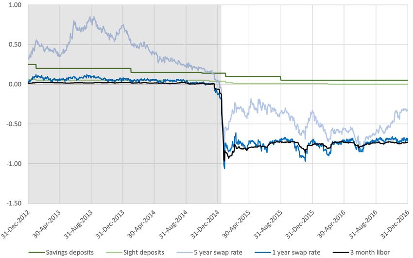
Lending rates Moving from market and deposit rates to corporate lending rates,
Figure 2 shows the average lending rates (upper panel) and lending spreads with re-
spect to Swiss government bonds (lower panel). In this figure, the sample of banks is
split into two groups: those with a deposit ratio above and below the median. Two ob-
servations stand out: First, lending rates moved relatively little following the monetary
policy rate cut, indicating incomplete interest rate pass-through. Since pass-through
to Swiss government bond yields was stronger and quicker, lending spreads with re-
spect to government bonds increased after the rate cut. Pass-through may have been
incomplete for a number of reasons, including heightened credit risk or market struc-
ture.
Our focus in this study will be on how a bank’s funding profile affects its response to
negative interest rates, controlling for other supply and demand factors. This brings us
to the second observation. There are notable differences between the two bank groups
in their responses to negative interest rates. High-deposit banks lowered spreads rel-
ative to low-deposit banks, i.e., interest pass-through was stronger.7 In the rest of the
paper, we will explore this stylized fact about the role of funding in more detail.
3.2 Empirical hypotheses
From a theoretical perspective, the combination of negative market rates and a lower
bound on deposit rates may affect transmission through three channels: the bank lend-
ing channel, the bank balance-sheet channel, and the risk-taking channel. Whereas the
bank lending and the bank balance-sheet channel could be weakened or reversed, the
risk-taking channel may be strengthened.
In particular, the bank lending channel (Bernanke and Blinder, 1988; Kashyap and
Stein, 1994) and its modern variant the deposit channel (Drechsler et al., 2017) suggest
that a policy rate cut leads to an increase in the volume of deposits. Since deposits are
a cheap source of funding, banks can expand their lending. However, Eggertsson et
al. (2019) argue that in a negative interest rate environment, the bank lending channel
collapses because deposit rates no longer respond to policy rate cuts.
According to the bank balance-sheet channel (Bernanke and Gertler, 1995; Gertler
and Kiyotaki, 2010), a monetary expansion increases bank net worth. Higher net worth
allows the bank to obtain better funding terms or relieves capital constraints. The
positive effect on net worth occurs because of maturity mismatches, with the value of
7
Note that the difference in levels prior to the rate cut (higher average rates for high-deposit banks)
is not a robust feature of the data and sensitive to the exact specification. In our preferred specification,
differences in levels will be absorbed by fixed effects.
88Figure 2: Monthly rolling average lending rates and spreads of high and low deposit
share banks
Notes: The lending rate is the interest rate charged on a loan at inception. The lending spread is defined
as the difference between the lending rate and the yield on a Swiss government bond with the same
maturity. Banks are split into two groups according to their deposit ratios. The deposit ratio is defined as
the sum of Swiss franc sight and savings deposits over total assets as of December 2014. Within the two
groups, 3-month rolling averages were calculated from our loan-level data set for a window of +/-360
days around the 15 January 2015 rate cut. Data sources are described in Section 4.1.
bank assets being less sensitive to interest rate changes than liabilities. In a negative
interest rate environment, the positive effect on net worth may be weakened or even
reversed, as deposit rates no longer respond to rate cuts and the value of liabilities
becomes less interest rate sensitive. Interest rate margins and profitability decrease
(Brunnermeier and Koby, 2018; Eggertsson et al., 2019), eventually lowering net worth
and constraining lending capacity. Hence, as a result of relatively higher funding costs,
we would expect high-deposit banks to lend less at higher interest rates.
According to the risk-taking channel (Borio and Zhu, 2012; Dell’Ariccia et al., 2014),
banks increase risk in response to rate cuts. Pennacchi and Santos (2018) and Alessan-
dri and Haldane (2009) provide evidence that banks target a specific level of return on
equity and that if their profitability falls, they increase risk-taking to maintain profits.
The risk-taking channel may be strengthened in a negative rate environment, either
because of informational frictions or behavioral biases.
Dell’Ariccia et al. (2014, 2017) provide a theoretical foundation for the risk-taking
99channel that relies on informational frictions and limited liability. In a positive rate
environment, there are two opposing effects of a rate cut. On the asset side, a re-
duction in the policy rate reduces the yield on safe assets, and banks increase their
demand for risky assets (portfolio rebalancing). On the liability side, profits typically
increase because of falling short-term funding costs. Due to limited liability, higher
profitability diminishes risk-taking incentives (risk-shifting). However, when rates are
negative, banks funded by deposits do not see their short-term funding costs fall, and
their profits will be under pressure. This reverses the moderating risk-shifting effect
and thereby amplifies the risk-taking channel. Put differently, when negative interest
rates are expected to last for a longer time, deposit funding effectively turns into a
fixed-rate liability, and banks may display a search-for-yield behavior similar to other
financial institutions with longer dated liabilities such as insurers, investment funds,
and pension funds (Rajan, 2005). In contrast to the bank lending and bank balance-
sheet channel mechanism, where marginal costs to expand the balance sheet change,
the intuition here is that banks try to make a profit with a given amount of deposit
funding at a given cost.8
On the behavioral side, Lian et al. (2018) provide experimental evidence that in-
vestors take on more risk when risk-free rates are low. That effect is considerably
stronger when interest rates are negative, consistent with prospect theory and loss
aversion (Kahneman and Tversky, 1979). This would mean that, with a positive inter-
est rate environment, a bank may be willing to accept a small margin for a safe project
(e.g., 0.1 basis points). With negative interest rates, however, due to loss aversion, it
will not invest in a project with a small negative margin but will prefer riskier projects
with a – non-risk-adjusted – positive margin.
In summary, theory leads to the following testable hypotheses on the role of deposits
when rates are negative. If the moderating (or reversing) effect of deposit funding on
the bank lending and bank balance-sheet channels dominates, we expect high-deposit
banks to lend less and at higher prices than their peers in response to a rate cut. If, on
the other hand, the risk-taking channel dominates, we expect high-deposit banks to
take more risks by a) attempting to expand their lending business by offering looser
terms and b) by granting loans to riskier firms.
In addition to deposit funding, the amount of excess liquidity that is subject to neg-
ative interest rates may have an effect on monetary transmission that is specific to a
negative rate environment (Basten and Mariathasan, 2018; Bottero et al., 2019). More
precisely, there is the possibility of portfolio rebalancing that would work similarly to
quantitative easing policies (Kandrac and Schlusche, 2017; Christensen and Krogstrup,
2018). Under portfolio rebalancing, banks adjust their portfolios towards assets with
a higher yield to avoid negative interest rates on central bank balances. Under that
hypothesis, we would expect banks with more charged reserves to grant more credit
at more attractive terms. Although it is not the main focus of the paper, we will discuss
8
The motivation for banks to move away from safe securities towards loans is also apparent in a
statement by the CEO of PostFinance, the Swiss postal bank, which relies mainly on deposit funding.
The law prohibits this bank from granting loans (see PostFinance, Annual Report Post 2017): ”[The fall
in revenue from the interest differential business] makes it clear that in the current negative interest rate
environment in particular, it is a serious disadvantage for us not to be able to issue our own loans and
mortgages. There is a need for action in this area, because our interest margin remains under pressure."
10
10this mechanism in Section 5.3.
4 Empirical strategy and data
4.1 Data
We use confidential loan-level data on nonfinancial corporate loans. Corporate loans
make up around a third of total domestic credit in Switzerland. We match these data
with individual bank balance-sheet information and regulatory reportings. All data
are collected by the SNB and publicly available only in aggregate form.
The corporate loan-level data are taken from the SNB lending rate statistic. For
each loan agreement, we have information on various lending terms (interest rate,
loan size, fixed or variable rate, commission, maturity, collateralization) and borrower
characteristics (sector, number of employees, location of headquarters). The statistic
also covers off-balance-sheet loan commitments. For each loan agreement, we know
the exact date when it was paid out. Importantly, loan commitments are recorded
when they are granted, not when they are first drawn upon.
The data cover all banks whose loans to nonfinancial domestic companies exceed
CHF 2 bn. Coverage is comprehensive, as the 20 banks that have to report their loans
grant approximately 80% of corporate loans in Switzerland. The banks are required
to report information on all new loan agreements with nonfinancial firms that exceed
CHF 50k in Swiss francs. New loan agreements comprise newly granted loans as well
as major modifications in conditions of existing loans.9 All reported loans have either
a fixed maturity of at least one month or are open ended. Banks report data from
mid-2006 onwards, and as of end 2017, the whole data set contained approximately 1.3
million loan agreements.
Our main source for bank balance-sheet information is the SNB monthly banking
statistic, which contains detailed information on the composition of banks’ assets and
liabilities. We combine this information with regulatory data on minimum reserves,
capital adequacy and liquidity.
To check whether our results also apply to other loan markets, we use data on resi-
dential mortgage loans. The data are from the SNB’s interest rate survey. Banks report
published end-of-month interest rates for new transactions. Our analysis focuses on
fixed residential mortgage rates for different maturities (one to ten years). This data
set differs from our corporate loan-level data set in several ways: first, banks report
published interest rates as opposed to actual loan transactions. Second, there is no
information about borrowers. Third, it covers a broader sample of banks than the
corporate loan data (45 banks).10 Therefore, the corporate loan-level data allow for a
more granular analysis, whereas the aggregate residential mortgage data set comprises
a larger number of banks. It also covers a larger share of overall credit (at end-2014,
residential mortgages accounted for approximately two-thirds of total domestic bank
9
Major modifications are defined as changes in loan terms that can be considered the result of a
renegotiation. In particular, new loan agreements include changes from a variable rate to a fixed rate,
prolongations of fixed-term loan contracts, and changes in ratings for open-ended contracts.
10
Banks whose total Swiss-franc-denominated customer deposits and cash bonds in Switzerland ex-
ceed CHF 500 million.
11Table 1: Loan characteristics: Descriptive statistics
N mean median std p1 p99
Data at individual loan level
lending spread (in pp) 109,420 2.494 1.939 1.622 0.478 7.278
interest rate (in pp) 109,420 2.161 1.550 1.544 0.460 6.750
log(loan size) (in CHF k) 109,420 6.162 5.991 1.409 3.912 9.908
loan size (in CHF mn) 109,420 1.695 0.400 6.154 0.050 22.915
fixed rate 109,420 0.619 1.000 0.486 0.000 1.000
commission 109,420 0.167 0.000 0.373 0.000 1.000
maturity (in years) 77,230 2.364 0.758 2.954 0.081 10.153
collateralized 109,420 0.809 1.000 0.393 0.000 1.000
High Risk Sector 109,420 0.276 0.000 0.447 0.000 1.000
Export Sector 109,420 0.044 0.000 0.205 0.000 1.000
Data at bank firm type level
vol. of new loan agreements (in CHF mn) 13,125 12.198 1.300 92.160 0.050 164.390
log(vol. of new loan agreements) (in CHF k) 13,125 7.299 7.170 1.844 3.912 12.010
Number of loans 13,125 7.005 2.000 24.365 1.000 78.000
log(avg. loan size) 13,125 6.227 6.064 1.295 3.912 9.903
log(Net Revenue)(in CHF k) 13,125 8.194 8.046 1.667 5.104 12.476
log(lending spread) (in pp) 13,125 0.893 0.874 0.592 -0.547 1.985
new firm-type post rate cut 6,881 0.072 0.000 0.258 0.000 1.000
exit firm-type post rate cut 13,964 0.027 0.000 0.162 0.000 1.000
Notes: The data are at the loan level and cover the period of a symmetric 180-day window around 15 January
2015. The lending spread is the interest rate charged at the beginning of the loan minus the risk-free rate
at the same maturity (as defined in Section 4.1); the loan size is the amount that is paid out or committed;
fixed rate is a dummy that takes a value of one if the interest rate was fixed over the maturity of the contract;
commission is a dummy that takes a value of one if a commission was charged on top of the interest rate; the
maturity of the loan is expressed in number of days divided by 360 (open-ended loan contracts not reported);
and collateralized is a dummy that takes a value of one if the loan was collateralized. High-risk sector is a
dummy that takes a value of one if the average lending spread (equally weighted across banks) in this sector
was above the median in the year before the rate cut (15 January 2014 to 14 January 2015); the dummy export
sector takes a value of one if the sector is in the top third of sectors by export intensity, which is defined as
a sector’s exports over its total output (as calculated by Egger et al. (2018).)
credit to the private sector).
4.2 Variables
4.2.1 Dependent variables
Descriptive statistics for the dependent variables are shown in Table 1.
Our first main variable of interest is the lending spread, which is defined as the
difference between the interest charged on a loan at inception and the yield on a Swiss
government bond with the same maturity (daily government bond yields are calculated
with a Nelson and Siegel (1987) term structure model). For variable rate loans, we use
the maturity of the base rate, and where the base rate is not reported, we assume a
maturity of 90 days. As a simpler measure of loan pricing, we also look at the lending
rate, i.e., without subtracting the risk-free rate.
The lending spread may be interpreted as an indicator for bank risk-taking when
1212firm risk is properly controlled for. As Paligorova and Santos (2017) argue, increased
risk appetite may manifest itself in a lower required compensation for risk, i.e., loan
spread. In the same vein, Ioannidou et al. (2015) point out that if granting riskier loans
is supply-driven, the average price per unit of risk should drop. In a theoretical model
by Martinez-Miera and Repullo (2017) with asymmetric information and costly mon-
itoring, lower spreads induce banks to monitor less, thereby increasing the riskiness
of their loan portfolios.
In addition to the lending spread, we look at the following relevant nonprice lending
terms:
• Loan size: If a bank grants a larger loan, it increases its exposure.
• Fixed/variable rate loan: If a bank grants more fixed rate loans, it increases du-
ration risk.
• Commission: A bank may try to offset lower lending spreads by demanding
higher commissions. Lepetit et al. (2008) found that banks may rely more on
fees to try to compensate for lower lending rates. Charging a commission in-
stead of a higher lending spread also decreases duration.
• Maturity: If a bank grants longer maturity loans, it takes on more risk since the
probability of unforeseen bad events over the life of the loan increases.11
• Collateralization: If the loan is collateralized, the bank takes on less risk, as the
losses in the event of default are smaller.
The continuous dependent variables are winsorized at the 1 percent level, grouped
by month.
All data above are at the individual loan level. In some specifications, we aggregate
the data to the bank/firm type level. This is described in Section 4.4.
4.2.2 Independent Variables
Descriptive statistics of the independent variables are shown in Table 2 and 3.
Our main independent variable is the ratio of Swiss franc deposits to total assets
(deposit ratio). Deposits are the sum of Swiss franc sight and savings deposits.
We include further balance-sheet characteristics to ensure that our results are not
driven by other banking characteristics. In our baseline specification, we employ
the following controls. The charged reserve ratio is the difference between Swiss
franc central bank deposits and the exemption threshold (see Section 3), i.e., the bank-
specific amount of deposits subject to negative interest rates. This ratio accounts for
the possibility of a portfolio rebalancing channel acting through the asset side of the
balance sheet (Basten and Mariathasan, 2018; Bottero et al., 2019). The total capital
ratio accounts for the bank capital channel of monetary policy and is defined as total
regulatory capital over total assets (Van den Heuvel, 2006). Finally, the log of total
assets controls for effects related to bank size (Stein and Kashyap, 2000).
11
We exclude all loans with open-ended maturity in these regressions. The number of observations is
therefore smaller.
13Table 2: Bank characteristics: Descriptive statistics
N mean median std p1 p99
Deposit Ratio 20 0.482 0.526 0.144 0.125 0.688
Charged Reserve Ratio 20 -0.045 -0.039 0.042 -0.145 0.043
log(Total Assets) (in CHF k ) 20 17.543 17.077 1.269 16.394 20.784
Capital Ratio 20 0.074 0.077 0.012 0.053 0.102
LCR 20 1.530 1.349 0.491 0.790 2.631
SME Loan Ratio 20 0.454 0.495 0.163 0.087 0.652
Net FX Pos./TA 20 -0.017 -0.011 0.027 -0.078 0.023
RoA (in pp) 20 0.245 0.243 0.087 0.075 0.401
Notes: The deposit ratio is defined as Swiss franc savings and sight deposits divided
by total assets; the charged reserve ratio is the reserves at the Swiss National Bank
subject to negative interest rates divided by total assets; the capital ratio is total reg-
ulatory capital divided by total assets; LCR is the regulatory liquidity coverage ratio;
Net FX Pos./TA is the net long position in foreign currency divided by total assets; the
SME loan ratio is loans and loan commitments to small and medium-size enterprises
divided by total loans; and RoA is the return on assets, i.e., profits divided by total
assets. All data are reported for December 2014.
In extensions, we look at the following further controls for bank characteristics. The
share of loans granted to small and medium enterprises (SMEs) to total assets accounts
for differences in business models. The FX ratio, defined as the net long position in
foreign currency (assets minus liabilities) divided by total assets, controls for possible
supply-side effects of currency mismatches. The regulatory liquidity coverage ratio
(LCR) and the loan-to-deposits ratio (total loans over total deposits) measure liquidity
position and funding model. The return on assets (RoA), defined as total profit over
total assets, captures the profitability of the banks.
For all bank characteristics, we use ex ante information to avoid endogeneity prob-
lems. Specifically, we take the latest value of the bank characteristic before the rate
change, i.e., as of 31 December 2014.
Table 3 compares the mean of bank characteristics of high-deposit banks (deposit
rate above median) with those of low-deposit banks (below median). Apart from the
deposit ratio itself (58 percent vs. 39 percent), we find no statistical differences in aver-
age bank characteristics, suggesting that these banks are not systematically different
in other dimensions.
We also explore heterogeneity across firms, in particular whether effects are differ-
ent for risky firms. To this end, we use two indicators. First, the “high risk sector”
indicator takes a value of one if the average lending spread (equally weighted across
banks) in this sector was above the median. To avoid endogeneity issues, we calculate
this indicator based on the year before the rate cut (15 January 2014 to 14 January
2015). Second, the “export sector” indicator takes a value of one if the sector is export
oriented. Firms in export-oriented sectors can be expected to have become relatively
riskier after the monetary policy decision, because the sudden exchange rate appre-
ciation made them less competitive. To identify export-oriented sectors, we rely on
Egger et al. (2018), who calculate export intensities based on OECD Inter-Country
Input-Output tables. Our indicator captures the top third of sectors by export inten-
sity, which is defined as a sector’s exports over its total output.
1414Table 3: Bank characteristics: High-deposit vs. low-deposit banks
Mean Mean
N Low Deposits High Deposits Difference t-Statistic p-Value
Deposit Ratio 20 0.388 0.575 -0.187 -3.817 0.001
Charged Reserve Ratio 20 -0.036 -0.054 0.018 0.941 0.359
log(Total Assets) (in CHF k ) 20 17.873 17.212 0.661 1.176 0.255
Capital Ratio 20 0.071 0.077 -0.006 -1.105 0.284
LCR 20 1.445 1.616 -0.171 -0.772 0.450
SME Loan Ratio 20 0.470 0.437 0.033 0.447 0.660
Net FX Pos./TA 20 -0.021 -0.013 -0.008 -0.674 0.509
RoA (in pp) 20 0.230 0.259 -0.029 -0.732 0.474
Notes: In this table, we compare average bank characteristics of banks with deposit ratios above the median
with those below the median. The deposit ratio is defined as Swiss franc savings and sight deposits divided by
total assets; the charged reserve ratio is the reserves at the Swiss National Bank subject to negative interest
rates divided by total assets; the capital ratio is total regulatory capital divided by total assets; LCR is the
regulatory liquidity coverage ratio; Net FX Pos./TA is the net long position in foreign currency divided by
total assets; the SME loan ratio is loans and loan commitments to small and medium-size enterprises divided
by total loans; and RoA is the return on assets, i.e., profits divided by total assets. All data are reported for
December 2014.
We also run a specification where we control for other lending terms (see above)
when analyzing the lending spread. Since these lending terms can be considered out-
come variables, this specification suffers from endogeneity problems. Nonetheless, it
may be helpful in detecting irregularities, e.g., if a lower spread is only due to better
collateralization.
4.3 Empirical Strategy
In general, analyzing the transmission of monetary policy through banks faces three
important challenges. First, market participants may anticipate policy rate moves and
thus frontload adjustments in their lending behavior. Moreover, policy rate decisions
may be made in response to domestic lending conditions, giving rise to endogeneity
issues. Second, lending supply and demand need to be disentangled. Third, demand
effects may vary across firms, calling for some level of granularity of demand controls.
To address these challenges, we base our identification on three pillars.
In our first pillar, we exploit the fact that the interest rate cut on 15 January 2015 was
unexpected, exogenous to the domestic economy, and large. Figure 1 shows that there
were no anticipation effects, as market rates suddenly dropped at the exact date of
the rate cut. This is important for our empirical strategy because our estimates would
likely underestimate the effect of the rate cut if it had been anticipated. Additionally,
anticipation would violate the common trends assumption behind the difference-in-
differences approach explained below.
Furthermore, as discussed above, the monetary policy move was a response to ex-
ogenous foreign developments. This alleviates any endogeneity concerns that arise if
the monetary policy decision was influenced by developments in the domestic lending
market.
The monetary policy decision on 15 January 2015 was clearly the most important
shock to market interest rates in the sample period we study. This is, for example,
15
15evident in Figure 1, where we observe large movements at the decision date, but not
before or afterwards. A large event ensures that our results are not driven by smaller
shocks before or after the monetary policy decision.
A possible concern is that the concurrent exchange rate appreciation had a sepa-
rate supply effect due to currency mismatches on bank balance sheets. This channel
is prominent in many emerging markets (Eichengreen and Hausmann, 1999). We con-
sider it unlikely that currency mismatches played an important role. No bank in our
sample reported large valuation losses or gains because of exchange rates in the three
subsequent years. This is probably because these banks had either small FX exposures
(median net FX long position: -1% of total assets) or were well hedged. In extensions,
we nonetheless add controls for currency mismatches.
Our second pillar is a difference-in-differences specification similar to that of Heider
et al. (2019). We compare lending i) before and after the rate cut and ii) between banks
with different deposit ratios. With this approach, we account for changes in demand
that are the same for all banks as well as time-invariant variation in the supply polices
of banks. A possible concern may be that banks change their operational efficiency.
For example, negative interest rates may be a trigger for high-deposit-share banks to
streamline their operations, allowing for lower spreads because of higher efficiency.
We do not directly control for this possibility but consider in extensions short horizons
where such an adjustment is very unlikely.
Our third pillar is the use of granular firm characteristics to control for changes in
credit demand specific to firm types. We follow a similar approach to Khwaja and Mian
(2008) and compare loan terms of multiple banks to the same firm type in the same
time period. The identification assumption is that when all banks grant a loan to the
same firm type, any differences in lending decisions are due to supply, i.e., bank char-
acteristics. Changes in a firm type’s credit demand or creditworthiness are absorbed
by the firm type*time fixed effect.
Granular firm controls are potentially important because demand effects are likely
to vary across firms because of the concurrent exchange rate appreciation. Efing et
al. (2015) show that export-oriented firms with costs primarily denominated in Swiss
francs suffered from larger declines in profits. If the composition of credit portfolios is
correlated with funding structure (e.g., if banks that lend to export-oriented firms rely
less on deposit funding), assuming only a common credit demand effect would bias
our results.
In addition, we use bank*firm type fixed effects to control for special lender-borrower
relationships. For example, some banks and firm types might keep long-standing rela-
tionships, which could result in systematically lower loan spreads (Boot, 2000). Alter-
natively, since some cantonal banks are legally required to promote lending to small
and medium-size enterprises in their home cantons, they might charge lower spreads
to these firm types.
Our data set contains detailed information on firm characteristics from which we
construct firm types (see Auer and Ongena, 2019, for a similar approach) as a combi-
nation of the borrowers’ sector (81 sectors), location (26 cantons, administrative divi-
sions in Switzerland) and number of employees (4 categories) and the time the loan
was granted (14 periods in our baseline).12 We require every firm type in a given pe-
12
We exclude all observations where an employee category is not reported, which is why the total
16
16riod to receive loans from at least two distinct banks. As a result of this restriction, our
sample is reduced to 7’074 distinct firm type*time fixed effects (72’573 observations).
On average, a firm type*time fixed effect has 3.0 relationships, with a maximum of
16 and a median of 2. There is some concentration in firm characteristics. For exam-
ple, approximately 29% of all observations in our baseline specification are in the real
estate sector, and approximately 14% of observations are in the canton of Zurich. In
robustness checks, we will verify that our results are not driven by these clusters.
Note that our data set does not contain unique firm identifiers; thus, we cannot
identify loans from multiple banks to the same firm, as in Khwaja and Mian (2008).
However, as Degryse et al. (2019) shows for Belgium, fixed effects that account for
variation in industry, location and firm size are sufficient to absorb firm-specific de-
mand effects. Moreover, this approach has the advantage that firms with only one
bank lending relationship are included. As the authors show, including singe-bank
firms can lead to vastly different bank credit supply shock estimates. These firms are
essential to properly account for supply movements when single-bank firms are abun-
dant. In the case of Belgium, 82% of firms are single-bank firms. Switzerland is similar
in this respect, with a share of single-bank firms of 75% (Dietrich et al., 2017).
4.4 Specification
Our simplest specification for the loan-level analysis takes the following form:
yl,b,f,t = βdepRatiob · Dt + α1 · Dt + α2 · depRatiob + l,b,f,t (1)
where yl,b,f,t is the lending spread (or an alternative lending term) charged on loan
l by bank b to firm type f paid out at date t (t measured in days).13 Dt is a dummy
indicating the period after the 15 January 2015 rate cut, and depRatiob is the ratio
of Swiss franc sight and saving deposits to total assets at the end of December 2014.
l,b,f,t is the error term.
The coefficient of interest is β. A negative β means that after the rate cut, banks with
a high deposit ratio lowered the lending spread more compared to banks with a low
deposit ratio. This indicates that reliance on deposit funding acts in an expansionary
way under negative interest rates, i.e., high-deposit banks loosen their lending terms
compared to low-deposit banks.
Starting from this simple specification, we successively add controls and increase
the granularity of the fixed effects. Our main regression specification takes the follow-
ing form:
yl,b,f,t = βdepRatiob ∗ Dt + γBCharb ∗ Dt + Ff,m + Fb,f + l,b,f,t , (2)
BCharb stands for other bank characteristics (size, capitalization, and charged re-
serves) that may affect the response to the rate cut. Ff,m are firm type*month fixed
effects, which control for firm type- and year-month-specific demand effects.14 Fb,f
number of observations is different from those reported in Table 2. Our main results are similar if we
treat “not reported” as a separate category.
13
A bank can grant multiple loans to a firm type in any period t.
14
More precisely, we additionally interact the firm type*year-month*Dt , effectively splitting the month
of January 2015 into a pre-rate cut and a post-rate cut period.
17
17are bank*firm type fixed effects to control for time-invariant unobserved bank hetero-
geneity by firm type. The sample period in the baseline covers the window between
180 days before and 180 days after the rate cut, with loans granted at the date of the
rate cut removed from the sample. In an extension, we will look at alternative window
sizes.
To explore whether the effects are more pronounced for risky firms, we run a sepa-
rate regression for risky sectors and other sectors. We implement this approach with
triple interactions:
yl,b,f,t = βdepRatiob ∗Dt +δdepRatiob ∗Riskf ∗Dt +Ff,m +Fb,f +l,b,f,t , (3)
where Riskf is an indicator function for the riskiness of the sector, as described in
Section 4.2.
Since at the loan level we only see the size of the loan but not the changes in the
number of loans granted to a specific firm type, we complement our analysis by ag-
gregating our loan-level data to the bank/firm level. This allows us to analyze whether
a bank changed loan quantities granted to a specific firm type (intensive margin) and
to check whether a bank entered new or terminated existing lending relationships
(extensive margin).
Specifically, for the analysis of the intensive margin, we sum up the size of the
individual loans to a given firm type in a given period, which gives us the volume of
new loan agreements at the firm type level.15 We look at two periods: the 180 days
before and after the rate cut. In addition to volume, we look separately at the average
loan size and the number of loans. For comparison purposes, we also consider the
average lending spread to a given firm type in a given period and net revenues from
credit intermediation, defined as the product of the lending spread and the volume of
new loan agreements. For each dependent variable, we end up with a two-period panel
of bank/firm types and apply the corresponding variant of equation (2). Note that due
to bank*firm type fixed effects, by design, we only include firm type/bank relations in
which a loan was granted in both periods.
For the extensive margin, we follow Khwaja and Mian (2008) and compute two sets
of dummies. One set designates newly created bank/firm type relationships (entry),
and the other designates bank/firm type relationships that were terminated (exit). Re-
garding entry, we check for each loan granted by a bank to a firm type after the rate
cut whether that bank has granted a loan to the same firm type in the previous five
years. If this is not the case, we interpret this as a newly formed relationship, and the
entry dummy equals one. Regarding exit, we check whether loan agreements granted
before the rate cut from a bank to a firm type expire after the rate cut. If that is the
case and no new loan is granted after the rate cut, the exit dummy equals one.16 For
the analysis of the extensive margin, the specification is again similar to equation 2,
15
As described above, new loan agreements cover new loans and major modification to existing con-
tracts, with no separate identification. For loan contracts with open-ended maturities, a change in the
bank internal rating is classified as a modification. To ensure that our results for lending volumes are
not driven by changes in the internal rating, we exclude loan contracts with open-ended maturities as a
robustness check. The results are not affected.
16
Since we have no information on when loans with open-ended maturities are paid back, we exclude
such loans from the exit analysis.
18
18You can also read